| Issue |
A&A
Volume 680, December 2023
|
|
|---|---|---|
| Article Number | A4 | |
| Number of page(s) | 15 | |
| Section | Extragalactic astronomy | |
| DOI | https://doi.org/10.1051/0004-6361/202143023 | |
| Published online | 04 December 2023 | |
A sensitive, high-resolution, wide-field IRAM NOEMA CO(1–0) survey of the very nearby spiral galaxy IC 342⋆
1
Observatorio Astronómico Nacional (IGN), C/Alfonso XII, 3, 28014 Madrid, Spain
e-mail: This email address is being protected from spambots. You need JavaScript enabled to view it.
2
Institut de Radioastronomie Millimétrique (IRAM), 300 Rue de la Piscine, 38406 Saint-Martin-d’Hères, France
3
Sorbonne Université, Observatoire de Paris, Université PSL, CNRS, LERMA, 75014 Paris, France
4
Max-Planck-Institut für extraterrestrische Physik, Giessenbachstraße 1, 85748 Garching, Germany
5
Department of Astronomy, The Ohio State University, 140 West 18th Avenue, Columbus, OH 43210, USA
6
Institut Laue-Langevin, 71 Avenue des Martyrs, 38042 Grenoble, France
7
Institute of Astronomy and Astrophysics, Academia Sinica, No. 1, Sec. 4, Roosevelt Road, Taipei 10617, Taiwan
8
Center for Astrophysics and Space Sciences, Department of Physics, University of California, San Diego, 9500 Gilman Drive, La Jolla, CA 92093, USA
9
Sterrenkundig Observatorium, Universiteit Gent, Krijgslaan 281 S9, 9000 Gent, Belgium
10
Department of Physics, University of Alberta, Edmonton, AB T6G 2E1, Canada
11
Max-Planck-Institut für Astronomie, Königstuhl 17, 69117 Heidelberg, Germany
12
Department of Physics and Astronomy, McMaster University, 1280 Main Street West, Hamilton, ON L8S 4M1, Canada
13
Canadian Institute for Theoretical Astrophysics (CITA), University of Toronto, 60 St George St, Toronto, ON M5S 3H8, Canada
14
Penn State Mont Alto, 1 Campus Drive, Mont Alto, PA 17237, USA
15
Argelander-Institut für Astronomie, Universität Bonn, Auf dem Hügel 71, 53121 Bonn, Germany
16
Universität Heidelberg, Zentrum für Astronomie, Institut für Theoretische Astrophysik, Albert-Ueberle-Str 2, 69120 Heidelberg, Germany
17
Cosmic Origins Of Life (COOL) Research DAO, coolresearch.io
18
European Southern Observatory, Karl-Schwarzschild Straße 2, 85748 Garching bei München, Germany
19
Univ Lyon, Univ Lyon 1, ENS de Lyon, CNRS, Centre de Recherche Astrophysique de Lyon UMR5574, 69230 Saint-Genis-Laval, France
20
Department of Physics, University of Connecticut, Storrs, CT 06269, USA
21
CNRS, IRAP, 9 Av. du Colonel Roche, BP 44346, 31028 Toulouse Cedex 4, France
22
Université de Toulouse, UPS-OMP, IRAP, 31028 Toulouse Cedex 4, France
23
Universität Heidelberg, Interdisziplinäres Zentrum für Wissenschaftliches Rechnen, Im Neuenheimer Feld 205, 69120 Heidelberg, Germany
24
Astronomisches Rechen-Institut, Zentrum für Astronomie der Universität Heidelberg, Mönchhofstraße 12-14, 69120 Heidelberg, Germany
25
Technical University of Munich, School of Engineering and Design, Department of Aerospace and Geodesy, Chair of Remote Sensing Technology, Arcisstr. 21, 80333 Munich, Germany
26
Department of Physics, Tamkang University, No. 151, Yingzhuan Rd., Tamsui Dist., New Taipei City 251301, Taiwan
27
Department of Astronomy & Astrophysics, University of California, San Diego, 9500 Gilman Drive, La Jolla, CA 92093, USA
Received:
31
December
2021
Accepted:
3
October
2023
Abstract
We present a new wide-field 10.75 × 10.75 arcmin2 (≈11 × 11 kpc2), high-resolution (θ = 3.6″ ≈ 60 pc) NOEMA CO(1–0) survey of the very nearby (d = 3.45 Mpc) spiral galaxy IC 342. The survey spans out to about 1.5 effective radii and covers most of the region where molecular gas dominates the cold interstellar medium. We resolved the CO emission into > 600 individual giant molecular clouds and associations. We assessed their properties and found that overall the clouds show approximate virial balance, with typical virial parameters of αvir = 1 − 2. The typical surface density and line width of molecular gas increase from the inter-arm region to the arm and bar region, and they reach their highest values in the inner kiloparsec of the galaxy (median Σmol ≈ 80, 140, 160, and 1100 M⊙ pc−2, σCO ≈ 6.6, 7.6, 9.7, and 18.4 km s−1 for inter-arm, arm, bar, and center clouds, respectively). Clouds in the central part of the galaxy show an enhanced line width relative to their surface densities and evidence of additional sources of dynamical broadening. All of these results agree well with studies of clouds in more distant galaxies at a similar physical resolution. Leveraging our measurements to estimate the density and gravitational free-fall time at 90 pc resolution, averaged on 1.5 kpc hexagonal apertures, we estimate a typical star formation efficiency per free-fall time of 0.45% with a 16 − 84% variation of 0.33 − 0.71% among such 1.5 kpc regions. We speculate that bar-driven gas inflow could explain the large gas concentration in the central kiloparsec and the buildup of the massive nuclear star cluster. This wide-area CO map of the closest face-on massive spiral galaxy demonstrates the current mapping power of NOEMA and has many potential applications. The data and products are publicly available.
Key words: Galaxy: general / Galaxy: disk / Galaxy: center / stars: formation / molecular data
Full Tables A.2 and A.3 and reduced datacubes are available at the CDS via anonymous ftp to cdsarc.cds.unistra.fr (130.79.128.5) or via https://cdsarc.cds.unistra.fr/viz-bin/cat/J/A+A/680/A4
© The Authors 2023
 Open Access article, published by EDP Sciences, under the terms of the Creative Commons Attribution License (https://creativecommons.org/licenses/by/4.0), which permits unrestricted use, distribution, and reproduction in any medium, provided the original work is properly cited.
This article is published in open access under the Subscribe to Open model. This email address is being protected from spambots. You need JavaScript enabled to view it. to support open access publication.
1. Introduction
Giant molecular clouds (GMCs) represent the immediate sites of star formation and set the boundary conditions for star formation (e.g., Kennicutt & Evans 2012). Far from universal, the properties of GMCs strongly depend on the local galactic environment (e.g., Gratier et al. 2010; Hughes et al. 2013; Colombo et al. 2014; Rosolowsky et al. 2021). In theory, the properties of molecular clouds play a key role in setting the rate at which molecular gas can form stars (e.g., Padoan et al. 2012; Federrath & Klessen 2013; Krumholz et al. 2019). These theoretical predictions have spurred a number of recent observational attempts to quantitatively link the properties of individual molecular clouds to the rate of star formation in galaxies or parts of galaxies (e.g., Barnes et al. 2017; Leroy et al. 2017; Ochsendorf et al. 2017; Hirota et al. 2018; Kreckel et al. 2018; Utomo et al. 2018; Schruba et al. 2019; Pessa et al. 2021).
To make such measurements, one must survey the properties of molecular gas with high resolution and high completeness across large parts of galaxies. Most often, this is done by observing low-J CO line emission, the standard tracer of molecular gas in galaxies (e.g., Bolatto et al. 2013). Though CO is among the brightest millimeter-wave lines, CO surveys still represent a major technical challenge, requiring a focused effort using the best millimeter and submillimeter telescopes in the world.
At a distance of only d = 3.45 Mpc (Anand et al. 2021), IC 342 represents one of the closest, massive, star-forming spiral galaxies beyond the Local Group (see Table 1). Among massive, vigorously star-forming disk galaxies, its proximity is rivalled only by Andromeda, NGC 253, and NGC 4945 and all of these systems are far more inclined than IC 342. This proximity and face-on orientation (i ∼ 30°) translate into a sharper physical resolution and less confusion due to galaxy projection across the entire electromagnetic spectrum. Even among nearby northern galaxies, IC 342 stands out as it is a prime example of a bulge-less spiral galaxy hosting a massive, compact nuclear star cluster (Carson et al. 2015; Neumayer et al. 2020) which is among the brightest ones known in nearby late-type galaxies (Georgiev & Böker 2014). Indeed, were it not for its position behind the Galactic plane (b = 10.6°), IC 342 would certainly be among the best-known galaxies in the sky. Even given this situation, the gas-rich nuclear region of IC 342 has been a key target of millimeter-wave studies for decades (e.g., Lo et al. 1984; Eckart et al. 1990; Downes et al. 1992; Sakamoto et al. 1999; Meier & Turner 2005; Pan et al. 2014). This rich region hosts one of the nearest nuclear star clusters that appears to heavily impact its surrounding gas reservoir (Schinnerer et al. 2003) and the nuclear region of IC 342 is one of the closest starbursts (we estimated a star formation rate inside the central 1.5 kpc equal to ∼ 0.2 M⊙ yr−1; see Sect. 2.2). Thus, there are some similarities with the less massive, very nearby galaxies M 33 and NGC 5253 regarding the presence of nuclear stellar clusters and nuclear starbursts. In any case, the proximity, orientation, and active star formation that allowed these earlier studies make IC 342 an ideal target for wider area CO surveys using more modern facilities.
Global properties of IC 342.
Here, we report on a new NOrthern Extended Millimeter Array (NOEMA) wide-area survey of CO emission of IC 342. We used NOEMA, supported by the IRAM 30-m telescope, to observe CO(1–0) emission from ∼1000 individual pointings across the inner region of IC 342. In total, we map 10.75 × 10.75 arcmin2, that is, about 11 × 11 kpc2, at an angular resolution of ∼3.6″ (or ∼60 pc). Here we describe this new survey, present a catalog of 637 molecular clouds from the galaxy, and compare their properties across different environments. We also assess how well environmental variations in the mean surface density of molecular clouds predict apparent variations in the molecular gas depletion time, testing some of the theoretical predictions described above.
IRAM NOEMA is the most powerful millimeter-wave interferometer in the northern hemisphere and one of the few telescopes in the world with the ability to conduct such CO surveys. With twelve 15-m dishes in the French Alps, recently upgraded receivers, and efficient observing, NOEMA can rapidly survey molecular line emission over hundreds or thousands of individual pointings. While the capabilities of ALMA are widely appreciated, NOEMA can survey CO emission at high completeness and high resolution from crucial northern targets such as the prototypical starburst M 82, the iconic spirals M 51 and M 101, the Local Group galaxies M 31 and M 33, and the “fireworks” galaxy NGC 6946 (all northern with d < 10 Mpc). The Plateau de Bure Interferometer, NOEMA’s predecessor, demonstrated these capabilities with the PAWS survey of M 51 (Schinnerer et al. 2013; Pety et al. 2013) and a 2–3 mm molecular line survey of NGC 6946 (Eibensteiner et al. 2022). Krieger et al. (2021) recently used NOEMA to produce a wide-field, high resolution map of CO emission in M 82, and Bešlić et al. (2021) mapped with NOEMA the J = 1 − 0 lines of two CO isotopologues (13CO and C18O) and of high critical density molecular tracers (HCN, HNC, and HCO+) towards the nearby strongly barred galaxy NGC 3627.
2. Data
2.1. Molecular gas surface density: The NOEMA survey
As part of project S16BF (P.I. A. Schruba), we observed the late-type spiral galaxy IC 342 for 120 h using eight antennas in the D configuration of NOEMA during the summer semester of 2016. A mosaic of 941 pointings was required to correctly sample the 10.75 × 10.75 arcmin2 targeted field of view. The short spacings that were filtered out by the interferometer were provided from observations with the IRAM 30-m telescope during 43 h in July 2016.
The data processing (calibration, merging, imaging, and deconvolution) followed the standard procedures of both observatories. Details are given in Appendix A. Briefly, data were calibrated using GILDAS/CLIC. We used reference quasars as phase and amplitude calibrators, and bright Galactic sources as flux calibrators. Around 20% of the data were flagged due to unstable weather. Imaging was carried out using GILDAS/MAPPING. First, we constructed pseudo-visibilities out of the IRAM 30 m data and they were merged with the NOEMA data in the uv plane using the task uvshort. The imaging process involved cleaning with the Högbom algorithm using a broad mask based on a smoothed and clipped version of the IRAM 30 m cube. The resulting data cube has an rms of 0.11 K over 5 km s−1 channels. We constructed data cubes with 5, 10, and 20 km s−1 spectral resolution. These three cubes were deconvolved separately. Because the deconvolution becomes more accurate when the signal-to-noise ratio of the data increases, we were able to deconvolve more flux in our 20 km s−1 resolution cube. The three cubes share the same angular resolution of 4 × 3.25 arcsec2 with a position angle of 91°. Table A.1 lists the salient features of the observations and reports the properties of our 5 km s−1 resolution data cube.
We compared the flux between the NRO 45 m data at 20″-resolution published in the Nobeyama CO Atlas of Nearby Spiral Galaxies (Kuno et al. 2007) with the IRAM 30 m data at 22.5″ resolution described here. We used the same channel spacing of 5 km s−1. We computed the flux in a field of view of 600″ × 600″ centered on the galaxy center and within the velocity range [ − 80, +140] km s−1. For a distance of 3.45 Mpc, we found a total luminosity of 7.04 and 7.00 K km s−1 pc2, for NRO and IRAM, respectively. The difference amounts to only 0.6%. We then compared the flux between the IRAM 30m data cube, the NOEMA+30 m combined cube, and the NOEMA-only cube. We here used the same channel spacing of 5 km s−1 and the same velocity range as above, but we restricted the field of view to 500″ × 500″ to avoid edge effects. We first regrid the 30 m data onto the NOEMA spatial grid, and we smoothed the NOEMA+30 m and NOEMA-only cubes to the spatial resolution of the 30 m data, that is, 22.5″. We found a luminosity of 6.20, 6.14, and 0.95 K km s−1 pc2 for the IRAM 30 m, NOEMA+30 m, and NOEMA-only cubes. The flux scales for the combined and single-dish data cubes thus agree within 1%. Only 15% of the total flux is recovered with the interferometer.
From the deconvolved data cubes, we produced a set of derived products including cubes with round beams at a series of fixed angular (5, 15, 21 arcsec) and physical (90, 150, 500, 1000, 1500 pc) resolutions, noise estimates, masks, and accompanying moment maps and uncertainties. The moment maps were produced using a dilated mask approach that follows the strategy presented in Leroy et al. (2022) which was applied to the products delivered for PHANGS-ALMA (Leroy et al. 2021a). Line widths were measured using the effective width approach (following Heyer et al. 2001), which is often more robust than second-order moment maps:  . Details are provided in Appendix B. Data cubes and associated data products are publicly available1.
The conversion from CO(1–0) integrated intensity to molecular gas surface density follows
 (1)
(1)
where αCO represents the conversion factor from CO(1–0) to H2 surface density (including a factor 1.36 to account for helium and heavier elements). The factor cos i corrects the surface densities for inclination. Throughout this paper, we apply a fixed αCO = 4.35 M⊙ pc−2 (K km s−1)−1 to IC 342 whenever converting from CO intensity to molecular gas mass or surface density. This value is appropriate for the Milky Way and typical of the disks of massive spiral galaxies (Bolatto et al. 2013). We do expect αCO to vary across IC 342, approaching a lower value in the center (e.g., Downes & Solomon 1998; Sandstrom et al. 2013; Chiang et al. 2021) and to anticorrelate with the known metallicity gradient of IC 342 (Pilyugin et al. 2014, and see Table 1). Recent dust-based analysis points to an αCO value in the central ∼kpc which is ∼4 times below the Galactic value (Chiang, priv. comm.; Chiang et al. 2023). According to Meier & Turner (2001) and Pan et al. (2014), in the central few hundred parsec of IC 342, αCO is ∼2–3 times lower than the Galactic value; Pan et al. (2014) suggest that the disk of IC 342 reaches αCO values two times above the Galactic αCO (albeit with significant fluctuations). This means that we can expect up to a factor of ∼5 bulk difference in αCO between disk and center. Based on this, we note the cases below where deviation from the adopted constant conversion factor likely influences our results.
2.2. Supporting data and measurements
We used VLA H I 21 cm line observations from Chiang et al. (2021) to trace neutral atomic gas. Specifically, we applied the following equation to transform H I observations to atomic gas surface density, which assumes optically thin 21 cm emission:
 (2)
(2)
where Σatom includes the 1.36 factor to account for helium and heavier elements. The cos i term again corrects for galaxy inclination.
We used a WISE 3.4 μm image to trace stellar mass and a WISE 22 μm image to estimate the local recent star formation rate (SFR) surface density (Wright et al. 2010). The WISE images were processed into an estimate of stellar mass following the procedures in Leroy et al. (2019); Leroy et al. (2021b). The WISE 3.4 μm image has significant contamination by foreground stars because IC 342 lies behind the Galactic plane. But since the only application of these data in this paper is large regional averages and radial profiles, we do not expect this to represent a large concern. The 22 μm image is not heavily affected by the Galactic foreground, and we proceed with the WISE 22 μm alone as our SFR tracer. We used the following prescription to convert the WISE 22 μm map to SFR:
 (3)
(3)
This prescription follows Leroy et al. (2021a) and assumes a Chabrier initial mass function (Chabrier 2003), which agrees with extinction-corrected Hα measurements of SFR from the PHANGS-MUSE survey (Belfiore et al. 2022) within ∼20 − 30%. In this case, we also use a Mayall MOSAIC Hα image kindly provided by Herrmann (priv. comm.) for a visual comparison.
We also made heavy use of an environmental “mask” based on the near-IR morphology of the galaxy following Querejeta et al. (2021). Appendix B.3 describes the construction of this mask in more detail and explains how we identify distinct “center”, “bar”, “arm”, and “inter-arm” regions.
We aggregated information from the cloud catalogs, SFR estimates, and molecular gas mass estimates into a set of regional property estimates. This aggregation follows the methods described in Sun et al. (2022) and resembles those deployed in Leroy et al. (2017) and Utomo et al. (2018). Briefly, we calculated the mass-weighted average of cloud properties as well as the aperture average of SFR and molecular gas surface densities in a series of 1.5 kpc hexagonal apertures, which together tile the entire footprint of the NOEMA+IRAM observations. Details about this data aggregation scheme can be found in Sun et al. (2022). We used these derived products to compare population-averaged estimates of the cloud gravitational free-fall time to the regional molecular gas depletion time. These measurements can be found in Table A.3.
3. Results
Figure 1 shows the molecular gas distribution as mapped by NOEMA+IRAM 30-m, together with the distributions of Hα line emission tracing gas ionized by young, massive stars (Herrmann, priv. comm.), and neutral atomic gas traced by the 21 cm line (Chiang et al. 2021). Together, these three tracers reveal an intricate network of multiple spiral arms that emanate from the bright center. The inner arms visible in CO emission and dominated by molecular gas appear prominent inside a galactocentric radius of 5 kpc. These molecular gas arms connect seamlessly to the outer arms traced by 21 cm emission and dominated by atomic gas, which can be traced all the way out to radii of ∼20 kpc. The ionized gas emission follows these spiral arms, showing a patchy distribution that reflects the presence of many individual H II regions and indicating that massive stars are actively forming along the gas arms.
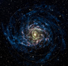 |
Fig. 1. Molecular, atomic, and ionized gas in IC 342. This is a false-color composite of IC 342 showing molecular gas traced by our new NOEMA CO(1–0) survey (green), along with stellar light from DSS2 (white), atomic gas traced by the 21 cm line using the VLA (blue), and Hα emission from ionized gas (red). The dashed rectangle delimits the field of view observed with NOEMA and solid ellipses show galactocentric radii at 5, 10, 15, and 20 kpc. |
Figure 2 shows our CO(1–0) survey in more detail. The top left panel illustrates the overall structure of CO emission in the galaxy for the observed field of view. Though the galaxy has been mapped before by lower-resolution, lower-sensitivity, or smaller field-of-view observations (including Crosthwaite et al. 2001; Helfer et al. 2003; Kuno et al. 2007; Hirota et al. 2011), the NOEMA map offers the sharpest, most complete view to date of the CO distribution in IC 342. The peak intensity map in Fig. 2 shows multiple spiral arms, fine inter-arm filaments, and a bright, elongated inner structure, which is reminiscent of gas lanes along a stellar bar and encompasses the nuclear starburst (e.g., Downes et al. 1992; Schinnerer et al. 2003; Meier & Turner 2005). The spiral arm east of the center has a significantly higher contrast similar to the (eastern) H I spiral arms further out in the disk (see Fig. 1). We speculate that this might be related to a mild interaction with a neighboring galaxy, which has also been evoked to explain the warping of the outer H I disk (e.g., Rots 1979; Crosthwaite et al. 2000; Stil et al. 2005). The CO velocity field shown in the top right panel follows a gentle S-shape which is consistent with streaming motions associated with a bar potential on top of a regularly rotating gas disk.
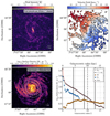 |
Fig. 2. NOEMA survey of CO(1–0) emission from IC 342. The distribution of the CO(1–0) peak intensity at the native angular resolution (top left) and the intensity-weighted mean CO velocity at 90 pc resolution (top right) as revealed by our new CO survey. The images show spiral arms, abundant inter-arm emission, and a velocity field that mostly reflects a regularly rotating gas disk. The bottom panels show the molecular gas traced by CO in the context of atomic gas and stars. In these panels, the CO and H I data are shown at a common ∼350 pc resolution. The bottom left panel shows a map of the total neutral gas surface density adding molecular gas surface density to atomic gas surface density from Chiang et al. (2021). The white ellipses show 1, 2, 3 × Re and the gray dashed ellipse indicates 1 R25. The lower right panel shows the azimuthally averaged mass surface density profiles for atomic gas, molecular gas, and stellar mass estimated from the near-infrared. The stellar mass distribution using HST imaging is consistent with a nuclear star cluster and an exponential disk (Carson et al. 2015), while the presented profile suffers from the resolution of the WISE data. Our NOEMA survey covers the inner molecule-dominated region where the H I emission is depressed, including the CO-bright center. |
The bottom row of Fig. 2 places our new CO survey in context. We combine the distribution of the atomic gas from Chiang et al. (2021) with our new molecular gas map at a matched resolution of ∼350 pc to show the total neutral gas surface density distribution (left panel) and to construct radial profiles of atomic gas, molecular gas, and stellar surface density (right panel). The effect of changing angular resolution is particularly apparent for the central bright molecular gas distribution where the position angle changes from a small offset to the east at ∼4″ resolution to a small western offset at 20″ resolution. This change is caused by lower surface brightness material outside the central 60″ which becomes apparent at the lower angular resolution. This might be a consequence of the bar in IC 342 (see Sect. 4).
The radial profiles show the basic distribution of the cold ISM in IC 342. Within 6 kpc, the molecular gas and stellar mass profiles have a nearly constant offset in logarithmic scale, implying a molecular gas to stellar fraction Σmol/(Σ⋆ + Σmol)≈0.20 − 0.25 for a constant Galactic αCO; if we assume a 2–3 times lower αCO in the center and twice higher αCO in the disk, as suggested by Pan et al. (2014), the molecular to stellar fraction would drop to ∼10% for the center and reach ∼40% throughout the disk. The molecular gas surface density exceeds the atomic gas surface density out to at least rgal = 6.7 kpc. Outside approximately this radius, the atomic gas dominates the cold ISM. As shown in Figs. 1 and 2, the structure of the molecular gas appears to connect smoothly with the atomic gas, consistent with a density- or pressure-dependent phase change. This large-scale picture agrees well with previous low-resolution work by Crosthwaite et al. (2001) and Pan et al. (2014). However, in contrast to previous work, our map captures the sharp concentration of gas at the galaxy center (rgal < 1 kpc) and resolves the CO emission from the galaxy into discrete molecular clouds. We explore the implications of these higher resolution observations in the next sections.
3.1. Giant molecular clouds in IC 342
We used the python implementation of the CPROPS algorithm (Rosolowsky & Leroy 2006) to generate a catalog of molecular clouds in IC 342. We apply the algorithm to the 90 pc and 5 km s−1 resolution cube and use the same methods developed by Rosolowsky et al. (2021) for the PHANGS-ALMA survey; see Appendix B.2 for details. These methods yield radius (R), line width (σ), and mass (M) for each cloud. We relied on the extrapolated and deconvolved GMC properties that account for the spatial and spectral response of NOEMA. When computing cloud radii, we followed  with η = 1.18 as in Rosolowsky et al. (2021). We adopted a fixed, Galactic αCO as stated above.
The CPROPS catalog contains 637 clouds with masses between 105 and 4 × 10⁷ M⊙ (out of which 602 have radius measurements). The catalog is publicly available2 and an excerpt showing the first ten rows can be seen in Table A.2. Given the θ = 90 pc resolution and this mass range, these objects likely span the range between giant molecular clouds and giant molecular associations. As we see below, they appear approximately gravitationally bound. Figure 3 visualizes their sizes and locations in the galaxy, with the clouds colored according to their dynamical environment (see Appendix B.3).
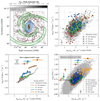 |
Fig. 3. Giant molecular clouds or associations in IC 342. The top left panel shows the location of the molecular clouds that we catalog at 90 pc resolution. The size of each circle corresponds to the deconvolved radius and the color indicates which dynamical environment the cloud is assigned to (red shows interarm clouds, green arm cloud, and blue center clouds). The top right and bottom left panels show the cloud properties in σ2/R vs. Σmol space, in which clouds with a fixed virial parameter follow a diagonal line with a slope of unity in log–log space. Σmol is the average surface density within the FWHM size of each cloud, Σmol = MCO/(2πR2). We show the IC 342 clouds for each environment and clouds at the same resolution and sensitivity, but better velocity resolution, from PHANGS-ALMA (Rosolowsky et al. 2021, and Hughes et al., in prep.). The bottom left panel replaces individual clouds with running medians. The bottom right panel adopts a beam-wise approach in which each independent line of sight at a fixed 90 pc resolution supplies a measurement of line width and surface density (Sun et al. 2018, 2020b). Again we compare the IC 342 points to those from a large sample of PHANGS-ALMA galaxies and here we mark the channel width and approximate sensitivity limit for the IC 342 data with dashed lines (for a Gaussian CO line, FWHM = 2.35σ, so we always have more than one channel across the FWHM of the emission line). The bottom row also indicates the mass-weighted median (position of the color circles) and 16 − 84% range (span of the color horizontal or vertical line) for surface densities and line widths. These refer to the corresponding horizontal or vertical axis, with an arbitrary positioning along the perpendicular direction. The mass-weighted averages tend to lie at higher values than the bulk of the individual measurements because much of the molecular gas mass resides in a few high-mass clouds or associations. All panels tell a consistent story: arm clouds show mildly enhanced surface density and line width compared to inter-arm clouds, and the center shows significant enhancements in surface density and line width. The elevated line widths in the center indicate high virial parameters suggesting clouds with additional contributions to their line widths. The deviations from self-gravity virialization would be even more extreme if we adopted a CO-to-H2 conversion factor below the Galactic value used to construct these plots. The black crosses in the right panels show representative error bars for our measurements in IC 342, as explained in the main text. |
The top right and bottom left panels of Fig. 3 illustrate the dynamical state of these molecular clouds using plots of σ2/R versus Σmol ≡ M/(2πR2) space. Following Heyer et al. (2009) and Field et al. (2011), variants of this plot have become a standard way to assess the properties of a molecular cloud population (e.g., see Leroy et al. 2015; Sun et al. 2018, 2020b; Rosolowsky et al. 2021). In the log–log plot of σ as a function of Σmol (bottom right panel), clouds with fixed virial parameter αvir = 2KE/UE, that is, a fixed ratio of kinetic energy (KE) to self-gravitating potential energy (UE), follow a straight line with slope of 1. Conversely, clouds with fixed turbulent pressure follow straight lines with slope of −1 (Sun et al. 2018, 2020b). Figure 3 shows the IC 342 clouds, separated by environment (as illustrated in the top left panel). As a reference we show a large set of GMC properties derived at identical spatial resolution and similar sensitivity from PHANGS-ALMA (Rosolowsky et al. 2021; Hughes et al., in prep.). We note that PHANGS-ALMA relies on the CO(2–1) transition, while the IC 342 observations presented here mapped CO(1–0); the ratio of both lines, R21, shows some mild variations within galaxies (e.g., den Brok et al. 2021; Leroy et al. 2022). The upper right panel shows individual clouds, while the lower left panel shows running medians in σ2/R as a function of Σmol. In the lower left panel, we plot the mass-weighted median and 16 − 84% range in surface density for each dynamical environment in IC 342.
In the bottom right panel of Fig. 3, we show a complementary view of the molecular ISM that captures similar information to the top right and bottom left panels. Here, we use a line-of-sight based approach following Sun et al. (2018; 2020b). We again take the θ = 90 pc data and now measure the intensity and line width along each line of sight. We sample the map using a hexagonal grid with spacing equal to the beam FWHM and consider only lines of sight where CO is detected over at least three 5 km s−1 channels. Then we show σ at this fixed spatial scale, which will be analogous to σ2/R for the clouds, as a function of Σmol, also at the fixed scale. Again we show results for PHANGS-ALMA, now from Sun et al. (2020b) for reference. Here we also plot the mass-weighted median and 16 − 84% range for each different environment. We plot typical error bars as the median fractional error associated with the NOEMA intensity map (14%) and linewidth map (18%) for Σmol and σ, respectively; we use a bootstrap approach (with N = 1000 iterations) for the uncertainty in σ2/R, taking the difference between the CPROPS radius with and without deconvolution as a representative error bar for R.
The two approaches and all three panels tell a consistent story. The clouds seen in IC 342 have properties broadly consistent with other clouds seen throughout the local galaxy population. Some of the flattening in line width at low surface density reflects the 2× coarser velocity resolution of the IC 342 data compared to PHANGS-ALMA (in gray). If we consider the dynamical state in only the high surface density, Σmol > 100 M⊙ pc−2 clouds, where the CO line is typically well-resolved by NOEMA, then we find a median virial parameter αvir = 2KE/UE ≈ 1.2 and 1.5 in the arm and inter-arm regions, respectively. The median virial parameter is higher (αvir ≈ 2.0) within the bar region, but then drops again for clouds in the very center (αvir ≈ 1.4). In any case, we find a range of virial parameters across environments (the global 16th–84th percentile range goes from 0.8 to 4.0, with a median αvir ≈ 1.6). As the figure shows, these arm and inter-arm results are well in-line with the PHANGS-ALMA clouds. The bar, on the other hand, shows enhanced σ2/R compared to arm or inter-arm values at matched molecular gas surface density. For the center, we note two subtleties. First, the highest surface density regions associated with the most massive clouds or pixels in the lower panels of Fig. 3 actually have αvir lower than 2.0, indicated by lower σ at fixed Σmol. In particular, the galaxy center itself appears, at our 90 pc resolution, roughly virialized, though we caution that 90 pc is quite coarse for such a study (e.g., see Schinnerer et al. 2006). Second, we caution that, as mentioned above, the center of IC 342 likely has a lower αCO than the Galactic value that we adopt (Israel 2020; Chiang et al. 2021). This will have the effect of moving the center points in all panels to the left, increasing their virial parameter by decreasing the surface density and thus the gravitational potential.
The surface density and line width increase moving from the inter-arm to the arm or bar, and then to the center regions. Weighting by mass, the median Σmol is ∼80, 140, 160, and 1100 M⊙ pc−2 for inter-arm, arm, bar, and center clouds, respectively, while the corresponding median line widths are 6.6, 7.6, 9.7 and 18.4 km s−1. The beam-by-beam statistics show similar trends, with mass-weighted median Σmol of 50, 80, 90, and 820 M⊙ pc−1 and mass-weighted median line widths of 5.2, 6.2, 7.7, and 17.2 km s−1 in the inter-arm, arm, bar, and center regions. According to Pan et al. (2014), αCO could be 2–3 times lower in what we define as the center region (innermost ∼kpc), which would lead to more moderate center surface densities (∼500 and ∼300 M⊙ pc−2 for GMCs and beam-by-beam, respectively). A two-sided Kolmogorov–Smirnov test confirms that the arm-interarm differences are statistically significant (p-value < 0.1%). At a similar level, the center is clearly different from the rest. The bar surface densities are not statistically distinct from the spiral arm values (p-value 36.8% for GMCs; 2.2% pixel-by-pixel), but bars do deviate from spiral arms in terms of σ2/R and σ (p-value < 0.1%).
Overall, these trends show an increase in surface density and line width moving from inter-arm to arm regions but with an approximately similar dynamical state. The center shows an increased surface density and line width. Many clouds in the central region, though not in the immediate center itself, show high line width relative to their surface density and evidence of broadening by forces other than self-gravity. A depressed αCO value would even emphasize this effect for the center. These results agree well with those found for larger populations of more distant galaxies in PHANGS-ALMA (Sun et al. 2020b; Rosolowsky et al. 2021).
3.2. Star formation efficiency per free-fall time
The rate at which stars form out of gas is often claimed to be primarily driven by gas density, which determines the local free-fall time, τff (e.g., see reviews in Lada & Lada 2003; Kennicutt & Evans 2012; Federrath & Klessen 2013; Padoan et al. 2014). Therefore, models of star formation often treat τff as a characteristic timescale for star formation, and express the fraction of gas converted to stars per gravitational free-fall time via ϵff = SFR/(Mmol/τff), a.k.a. the “efficiency per free-fall time” (e.g., McKee & Ostriker 2007; Krumholz et al. 2019). Some work has suggested ϵff to be approximately constant across a wide range of scales and systems, so that density variations represent a main physical driver of variations in the molecular gas depletion time (e.g., see Krumholz & Thompson 2007; Krumholz et al. 2019). In other work, ϵff represents a key quantity but varies depending on the local physical state of the gas (e.g., Utomo et al. 2018; Sun et al. 2023).
We estimated the molecular cloud free-fall time τff in IC 342 from our high-resolution CO data. Our CPROPS analysis provides measurements of mass and size for each identified molecular cloud. From these measurements, we estimated the mean volume density via ρ = 3M/4πR3 and the associated gravitational free-fall time via  . We then averaged over all clouds in each 1.5 kpc-diameter hexagonal region of IC 342, calculating the mass-weighted mean reciprocal of τff via
 (4)
(4)
where i is the index of clouds in that kpc-sized aperture. We follow Utomo et al. (2018) and Sun et al. (2022, 2023) in calculating the mass-weighted harmonic mean of τff, which ensures that the result is representative of the free-fall time for the entire cloud population in each hexagonal aperture. This ensures that ⟨τff⟩−1 is the correct quantity to compare to  to test the hypothesis of fixed ϵff. We estimated typical error bars on our measurements following a bootstrap approach with N = 1000 iterations. Within each hexagonal aperture, we perturbed the surface density and radius of each cloud following a Gaussian with standard deviation equal to 14% of each cloud’s surface density and 16% of its radius, which are the typical error bars that we have derived across our sample. In each iteration, we recomputed ρ and τff for each cloud with these perturbed values, and calculated the mass-weighted average of
  within each hexagonal aperture. Based on these 1000 iterations, we obtained the fractional error on τff for each aperture, and computed the median across all apertures, which is 6%. For
  , we assume the same 14% typical uncertainty on Σmol and take the median difference between the SFR calculated from WISE 4 and WISE 3 (17%) as a representative error bar. These combine to yield a typical error bar of 22% for
  .
.
The median ⟨τff⟩ in our sample of regions is 11 Myr with a 16 − 84% range of 8.5 − 14.8 Myr. This is slightly longer than the median value of  found for other galaxies at this scale by Rosolowsky et al. (2021), but still in agreement within 2σ given the measured galaxy-to-galaxy variation. For comparison, Kim et al. (2021), also using these data, made a statistical estimate of the cloud lifetime in IC 342 and found ∼20 Myr. This implies that clouds live ∼2τff in this galaxy, in good agreement with the results of Kruijssen et al. (2019), Chevance et al. (2020), and Kim et al. (2022) for a broader sample of galaxies.
In addition to ⟨τff⟩, we also calculated the integrated molecular gas depletion time,  , in each region via
 (5)
(5)
Here, Mmol and SFR are the integrated molecular gas mass and star formation rate in that aperture (measured from WISE 22 μm using Eq. (3)). A high  corresponds to a low rate of star formation per unit molecular gas and implies that star formation will take a long time to consume the available gas reservoir.
We combined ⟨τff⟩ and  to estimate the mean efficiency per free-fall time in that aperture via
  . By using 1.5 kpc-sized apertures, we average over many clouds at different evolutionary stages, which makes our results robust to stochasticity and the evolutionary state of individual clouds. This approach follows similar work by Leroy et al. (2017), Utomo et al. (2018) and Schruba et al. (2019), and the hexagonal sampling scheme and measurements follow Sun et al. (2020a).
In Fig. 4, we compare ⟨τff⟩ and  for each 1.5 kpc region. Each hexagon symbol shows results for one aperture, with the points color-coded according to the deprojected galactocentric radius at the aperture center. The red line shows the expectation for τdep = ⟨τff⟩/ϵff at the median measured ϵff and the pink region shows the 16 − 84% range of estimated ϵff. If ϵff is indeed constant and if density variations drive variations in
  then we would expect the data to follow that red line.
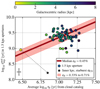 |
Fig. 4. Star formation efficiency per gravitational free-fall time in 1.5 kpc regions. Each hexagonal point shows the integrated molecular gas depletion time for a 1.5 kpc diameter region as a function of the mass-weighted average τff (see Eq. (4)) for 90 pc resolution clouds in that region. A straight, diagonal line in this space, such as the dark red one, corresponds to a fixed ϵff, which could be expected if density variations represent the primary drivers of depletion time variations. We color the regions by galactocentric radius and calculate the implied ϵff for each region. We estimate a median ϵff of 0.45% with a 16 − 84% range of 0.33 − 0.71%, and we illustrate these with the solid red line and shaded pink region. For the central 1.5 kpc region, we illustrate the effect of switching from our adopted Galactic αCO to a starburst conversion factor. The black cross shows a representative error bar as explained in the main text. The plotted values can be found in Table A.3. |
For our 90 pc resolution cloud catalog and using CO(1–0) with a fixed conversion factor and our WISE 22 μm-based SFR estimates, we find a median of ϵff = 0.45% with a 16 − 84% range of 0.33 − 0.71%. This value is near the frequently invoked value of 0.5% (e.g., McKee & Ostriker 2007) and broadly consistent with previous estimates in the literature (e.g., Vutisalchavakul et al. 2016; Barnes et al. 2017; Leroy et al. 2017; Utomo et al. 2018; Schruba et al. 2019). In detail, the value is towards the low end of the distribution for PHANGS-ALMA galaxies found by Utomo et al. (2018) and intermediate between their 0.7% mean value and the 0.3% found at 40 pc resolution for PAWS by Leroy et al. (2017). All of these values tend to be somewhat lower than those found for Galactic objects.
We can wonder if our IC 342 measurements support the idea of a fixed ϵff. On one hand, within the disk of the galaxy, that is, excluding the central aperture, there does not appear to be any significant relation between ⟨τff⟩ and  . The Spearman’s rank correlation relating the two is about −0.14, which goes opposite the predicted direction for a constant ϵff, and the relationship has an insignificant p-value of 0.26. The disk of IC 342 appears to exhibit a similar value of ϵff to other cases, but any internal changes in
  do not show clear evidence of being driven by density variations.
On the other hand, the contrast between the central 1.5 kpc averaged measurement, indicated by a bright yellow hexagon, and the cloud of regions in the disk does offer some support for the ideas that ϵff is fixed and that density variations drive  variations. Unfortunately, for the center, αCO complicates the picture. We have adopted a single fixed αCO for Fig. 4 but expect that the center, at least, shows a depressed αCO. For instance, Meier et al. (2011), Pan et al. (2014), Israel (2020), and Chiang et al. (2021), all find low αCO for the inner part of IC 342. This can have a dramatic effect on ϵff, which we illustrate by also plotting results for the central 1.5 kpc of IC 342 using a “starburst” αCO = 0.8 M⊙ pc−2 (K km s−1)−1 conversion factor (Downes & Solomon 1998; Bolatto et al. 2013). We do not expect αCO to be necessarily this low in the center of IC 342, but this implies a difference of a factor of ∼5 between center and disk, which is probably realistic. For example, Pan et al. (2014) found a central αCO 2–3 below the Galactic value, while for the disk αCO was found to be typically two times above the Galactic value, amounting to a similar difference of a factor ∼5. Applying this five times lower αCO in the center implies a significantly higher ϵff for the central region, ∼4.2% instead of 0.3%. This suggests that ϵff varies between the disk and the central region and highlights the importance of accurate αCO to these estimates.
4. Discussion: Central molecular gas reservoir and nuclear star cluster
Figure 5 shows three zooms of the IC 342 center after deprojection of its inclination on the plane of sky. Several properties of IC 342’s central region are similar to those in our Milky Way: the high molecular gas concentration, its geometry, and the massive nuclear star cluster (NSC, e.g., Schinnerer et al. 2003; Neumayer et al. 2020). A striking feature of the new CO map is the sharp increase in molecular gas surface density in the central ∼1 kpc (see Fig. 2). The average molecular mass surface density in the central 1.5 kpc measured at 90 pc resolution is about 600 M⊙ pc−2 (for a Galactic αCO), that is, a factor of 10× higher than in the immediate surroundings. Such sharp contrasts in CO surface brightness between center and disk are only seen in nearby galaxies that host a prominent stellar bar (see, e.g., CO atlas from PHANGS-ALMA, Leroy et al. 2021b).
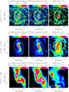 |
Fig. 5. Zooms of the molecular surface density, peak temperature, and line width towards the galaxy center. The images have been deprojected from the galaxy inclination on the plane of sky, and then converted to kpc using a distance of 3.45 Mpc. The yellow lines show our spiral mask, while the red and white ellipses delimit the extent of the bar and center environment, respectively (see Appendix B.3 for the definition of these environment). |
The non-axisymmetric gas morphology in the center appear related to the underlying dynamical structure in IC 342. However, the existence of a stellar bar in IC 342 has been debated in the literature. Buta & McCall (1999) did not discuss a potential bar, but they carried out ellipse fitting of V and I band images that shows changes in position angle and ellipticity which we find suggestive of a large-scale bar component. Based on ellipse fitting of deep near infrared images, Fathi et al. (2009) reported a large-scale stellar bar of 307″ (or ∼5.1 kpc) semi-major axis oriented roughly north–south, while Hernandez et al. (2005) found the bar to be not well-defined. Crosthwaite et al. (2000) reported evidence for a “fat” or “boxy” bar potential based on the analysis of their H I kinematic data.
We examined high-quality NIR imaging from Spitzer IRAC 3.6 μm and found clear evidence for the presence of a stellar bar with semi-major length of 120″ (or ∼2 kpc) and an orientation of PA = 160° (Appendix B.3). In addition to this photometric evidence, the presence of a bar is also suggested by CO morphology in the central 60″ (see for a summary and sketch Meier & Turner 2005). The distribution of the CO line emission shows two slightly curved gas lanes ending towards the center in a ring-like shape which coincides with a ∼100 pc diameter star-forming pseudoring (or nuclear spiral), and shock tracers appear preferentially on the leading sides of the lanes close to where they connect to the ring (a morphology that is clearly revealed by our data, see Fig. 5.). In the whole PHANGS-ALMA CO morphology catalog, such a setup is only observed in barred galaxies (Stuber et al. 2023). Moreover, CO morphology suggests that it is a relatively weak bar, because the bar lanes are curved and do not extend all the way out to the bar ends (e.g., Athanassoula 1992; Comerón et al. 2009). The CO kinematics are also consistent with the gas responding to an underlying non-axisymmetric (bar) potential. The presence of bar lanes is also supported by observations of the magnetic field (Beck 2015). Finally, the NSC in IC 342 is at the same time extremely massive and compact – consistent with a picture where bar-driven gas inflow triggers in situ star formation that drives the stellar densities in NSCs to extremely high values (Neumayer et al. 2020; Pechetti et al. 2020).
In this paper, we have presented measurements showing elevated gas velocity dispersion within the center environment (Sect. 3.1). The current central gas concentration and bar lanes, which are connected to a pseudoring (or nuclear spiral), can be interpreted as a consequence of that high velocity dispersion. Indeed, theoretical studies suggest that local gas properties such as the effective sound speed play a key role in determining the gas morphology within bars, beyond the existence or not of an inner Lindblad resonance (ILR; e.g., Englmaier & Gerhard 1997; Englmaier & Shlosman 2000; Sormani et al. 2018). The expectation is that warmer gas with high velocity dispersion (higher sound speed) will result in a more open nuclear spiral, which also critically depends on the central mass concentration.
Simulations show that the morphology of these central gas structures varies quickly over time (e.g., Emsellem et al. 2015; Renaud et al. 2015; Sormani et al. 2020). Therefore, the present configuration is probably not long-lived and was different in the past. We speculate that there might have been a stable nuclear ring associated with the bar in the past, which prevented gas inflow; the gas in this ring could have experienced dynamical and thermal heating due to feedback, giving way to the current open spiral morphology. This could signify that gas has only recently been able to reach the center, where it could contribute to the growth of the massive NSC. This process could have occurred intermittently, tied to rapid changes in the central gas morphology (i.e., from ring to open spiral and back again) that lead to periodic gas inflow to the center. In this case, bar-driven inflow episodes like this over the course of IC 342’s recent history would be responsible for building the NSC. Indeed, the nuclei of barred galaxies typically host much more elevated gas surface densities than unbarred galaxies (e.g., Sakamoto et al. 1999; Sun et al. 2020a). It should be kept in mind, however, that it is difficult to determine precisely the past evolutionary history from the present gas distribution (Renaud et al. 2015; Sormani et al. 2020).
5. Conclusions
We have presented a new, large, sensitive, ∼1000-pointing CO(1–0) line mosaic of the very nearby galaxy IC 342, carried out using the IRAM NOEMA and 30-m telescopes. The survey covers the inner ∼11 × 11 kpc2 region, which corresponds to roughly 1.5 effective radii and extends out to near the radius where the galaxy becomes atomic gas dominated. With a linear resolution of ∼60 pc, our beam is about the size of a massive giant molecular cloud. We resolve the galaxy into a series of bright spiral arms, inter-arm filaments, and the well-known bright central molecular structure which is consistent with gas flowing along a stellar bar. The well-known bright starburst center of IC 342 appears prominent in all of our data products.
We applied the CPROPS algorithm to identify > 600 massive molecular objects that are either molecular clouds or molecular associations. We did this at 90 pc resolution, so that IC 342 can be placed in the context of a large set of molecular cloud properties recently measured by PHANGS-ALMA. We also conducted a parallel “beam-wise” analysis in which we estimated the line width and molecular surface density for each independent line of sight where CO is detected over at least three consecutive channels. Both analyses highlight that the surface density and line width increase from the inter-arm region to the arm and bar region, and gas in the center of the galaxy has the highest surface density and line width. For clouds, we find a mass-weighted median Σmol ≈ 80, 140, 160, and 1100 M⊙ pc−2, and σCO ≈ 6.6, 7.6, 9.7 and 18.4 km s−1 for inter-arm, arm, bar, and center, respectively. Our beam-by-beam statistics yield similar results, Σmol ≈ 50, 80, 90, and 820 M⊙ pc−1, and σCO ≈ 5.2, 6.2, 7.7, and 17.2 km s−1, respectively. A 2 − 3 times lower αCO in the center yields median surface densities of ∼500 and ∼300 M⊙ pc−2 for GMCs and beam-by-beam, respectively. Moreover, for a Galactic αCO clouds appear to be in rough virial equilibrium in both the cloud-based and “beam-wise” analysis. The clouds in the bar and central region show elevated line widths, consistent with dynamical broadening by forces other than self-gravity and in good agreement with previous observations of galaxy centers using both techniques. If we had adopted a lower conversion factor, as is likely appropriate for the inner region, the dynamical state of the gas in the center would depart even more from simple virial equilibrium where turbulence balances self-gravity.
We used the cloud properties measured at 90 pc resolution to estimate the density, gravitational free-fall times, and star formation efficiency per free-fall time. We find median ⟨τff⟩≈11 Myr and ϵff = 0.45% on average with a 16 − 84% range of 0.33 − 0.71%. This is in agreement with literature estimates of this quantity, though towards the low end of such estimates. The center shows shorter molecular gas depletion time and gravitational free-fall time. Whether it has the same ϵff compared to the disk depends sensitively on the adopted αCO. Combining these values with recent statistical estimates of the GMC lifetime in IC 342 implies that clouds in the galaxy live for typically ∼2 times the free-fall time.
Given the proximity of IC 342, the CO observations and GMC catalog presented in this paper could have a wide range of applications for studies of the nearby universe. The data, along with our data products, are publicly available.
See http://www.iram.fr/IRAMFR/GILDAS for more information about the GILDAS softwares.
Acknowledgments
We thank the anonymous referee for a very constructive report. We gratefully acknowledge support from the NOEMA observatory staff. M.Q. acknowledges support from the Spanish grant PID2019-106027GA-C44, funded by MCIN/AEI/10.13039/501100011033. J.P. acknowledges support by the Programme National “Physique et Chimie du Milieu Interstellaire” (PCMI) of CNRS/INSU with INC/INP, co-funded by CEA and CNES. E.S. and T.G.W. acknowledge funding from the European Research Council (ERC) under the European Union’s Horizon 2020 research and innovation programme (grant agreement No. 694343). J.S. acknowledges support by the Natural Sciences and Engineering Research Council of Canada (NSERC) through a Canadian Institute for Theoretical Astrophysics (CITA) National Fellowship. M.C. and J.M.D.K. gratefully acknowledge funding from the DFG through an Emmy Noether Grant (grant number KR4801/1-1), as well as from the European Research Council (ERC) under the European Union’s Horizon 2020 research and innovation programme via the ERC Starting Grant MUSTANG (grant agreement number 714907). M.C. gratefully acknowledges funding from the DFG through an Emmy Noether Grant (grant number CH2137/1-1). COOL Research DAO is a Decentralised Autonomous Organisation supporting research in astrophysics aimed at uncovering our cosmic origins. M.C., J.K., and J.M.D.K. gratefully acknowledge funding from the German Research Foundation (DFG) through the DFG Sachbeihilfe (grant number KR4801/2-1). C.E. gratefully acknowledges funding from the Deutsche Forschungsgemeinschaft (DFG) Sachbeihilfe, grant number BI1546/3-1. K.K. gratefully acknowledges funding from the German Research Foundation (DFG) in the form of an Emmy Noether Research Group (grant number KR4598/2-1). R.S.K. acknowledges financial support from the European Research Council (ERC) via the ERC Synergy Grant “ECOGAL” (grant 855130) as well as from the Heidelberg cluster of excellence EXC 2181 (Project-ID 390900948) “STRUCTURES” funded by the German Excellence Strategy. R.S.K. also thanks DFG for support via the collaborative research center (SFB 881, Project-ID 138713538) “The Milky Way System” (subprojects A1, B1, B2, and B8).
References
- Anand, G. S., Lee, J. C., Van Dyk, S. D., et al. 2021, MNRAS, 501, 3621 [Google Scholar]
- Aniano, G., Draine, B. T., Hunt, L. K., et al. 2020, ApJ, 889, 150 [NASA ADS] [CrossRef] [Google Scholar]
- Athanassoula, E. 1992, MNRAS, 259, 345 [Google Scholar]
- Barnes, A. T., Longmore, S. N., Battersby, C., et al. 2017, MNRAS, 469, 2263 [Google Scholar]
- Beck, R. 2015, A&A, 578, A93 [NASA ADS] [CrossRef] [EDP Sciences] [Google Scholar]
- Belfiore, F., Santoro, F., Groves, B., et al. 2022, A&A, 659, A26 [NASA ADS] [CrossRef] [EDP Sciences] [Google Scholar]
- Bešlić, I., Barnes, A. T., Bigiel, F., et al. 2021, MNRAS, 506, 963 [CrossRef] [Google Scholar]
- Bolatto, A. D., Wolfire, M., & Leroy, A. K. 2013, ARA&A, 51, 207 [CrossRef] [Google Scholar]
- Buta, R. J., & McCall, M. L. 1999, ApJS, 124, 33 [NASA ADS] [CrossRef] [Google Scholar]
- Carson, D. J., Barth, A. J., Seth, A. C., et al. 2015, AJ, 149, 170 [Google Scholar]
- Chabrier, G. 2003, PASP, 115, 763 [Google Scholar]
- Chevance, M., Kruijssen, J. M. D., Hygate, A. P. S., et al. 2020, MNRAS, 493, 2872 [NASA ADS] [CrossRef] [Google Scholar]
- Chiang, I.-D., Sandstrom, K. M., Chastenet, J., et al. 2021, ApJ, 907, 29 [NASA ADS] [CrossRef] [Google Scholar]
- Chiang, I.-D., Hirashita, H., Chastenet, J., et al. 2023, MNRAS, 520, 5506 [CrossRef] [Google Scholar]
- Colombo, D., Hughes, A., Schinnerer, E., et al. 2014, ApJ, 784, 3 [NASA ADS] [CrossRef] [Google Scholar]
- Comerón, S., Martínez-Valpuesta, I., Knapen, J. H., & Beckman, J. E. 2009, ApJ, 706, L256 [CrossRef] [Google Scholar]
- Crosthwaite, L. P., Turner, J. L., & Ho, P. T. P. 2000, AJ, 119, 1720 [CrossRef] [Google Scholar]
- Crosthwaite, L. P., Turner, J. L., Hurt, R. L., et al. 2001, AJ, 122, 797 [NASA ADS] [CrossRef] [Google Scholar]
- den Brok, J. S., Chatzigiannakis, D., Bigiel, F., et al. 2021, MNRAS, 504, 3221 [NASA ADS] [CrossRef] [Google Scholar]
- Downes, D., & Solomon, P. M. 1998, ApJ, 507, 615 [NASA ADS] [CrossRef] [Google Scholar]
- Downes, D., Radford, S. J. E., Guilloteau, S., et al. 1992, A&A, 262, 424 [NASA ADS] [Google Scholar]
- Eckart, A., Downes, D., Genzel, R., et al. 1990, ApJ, 348, 434 [NASA ADS] [CrossRef] [Google Scholar]
- Eibensteiner, C., Barnes, A. T., Bigiel, F., et al. 2022, A&A, 659, A173 [CrossRef] [EDP Sciences] [Google Scholar]
- Emsellem, E., Renaud, F., Bournaud, F., et al. 2015, MNRAS, 446, 2468 [Google Scholar]
- Englmaier, P., & Gerhard, O. 1997, MNRAS, 287, 57 [NASA ADS] [Google Scholar]
- Englmaier, P., & Shlosman, I. 2000, ApJ, 528, 677 [NASA ADS] [CrossRef] [Google Scholar]
- Fathi, K., Beckman, J. E., Piñol-Ferrer, N., et al. 2009, ApJ, 704, 1657 [NASA ADS] [CrossRef] [Google Scholar]
- Federrath, C., & Klessen, R. S. 2013, ApJ, 763, 51 [Google Scholar]
- Field, G. B., Blackman, E. G., & Keto, E. R. 2011, MNRAS, 416, 710 [NASA ADS] [Google Scholar]
- Georgiev, I. Y., & Böker, T. 2014, MNRAS, 441, 3570 [Google Scholar]
- Gratier, P., Braine, J., Rodriguez-Fernandez, N. J., et al. 2010, A&A, 522, A3 [NASA ADS] [CrossRef] [EDP Sciences] [Google Scholar]
- Helfer, T. T., Thornley, M. D., Regan, M. W., et al. 2003, ApJS, 145, 259 [NASA ADS] [CrossRef] [Google Scholar]
- Hernandez, O., Wozniak, H., Carignan, C., et al. 2005, ApJ, 632, 253 [NASA ADS] [CrossRef] [Google Scholar]
- Herrera-Endoqui, M., Díaz-García, S., Laurikainen, E., & Salo, H. 2015, A&A, 582, A86 [NASA ADS] [CrossRef] [EDP Sciences] [Google Scholar]
- Heyer, M. H., Carpenter, J. M., & Snell, R. L. 2001, ApJ, 551, 852 [NASA ADS] [CrossRef] [Google Scholar]
- Heyer, M., Krawczyk, C., Duval, J., & Jackson, J. M. 2009, ApJ, 699, 1092 [Google Scholar]
- Hirota, A., Kuno, N., Sato, N., et al. 2011, ApJ, 737, 40 [NASA ADS] [CrossRef] [Google Scholar]
- Hirota, A., Egusa, F., Baba, J., et al. 2018, PASJ, 70, 73 [CrossRef] [Google Scholar]
- Hughes, A., Meidt, S. E., Colombo, D., et al. 2013, ApJ, 779, 46 [NASA ADS] [CrossRef] [Google Scholar]
- Israel, F. P. 2020, A&A, 635, A131 [NASA ADS] [CrossRef] [EDP Sciences] [Google Scholar]
- Kennicutt, R. C., & Evans, N. J. 2012, ARA&A, 50, 531 [NASA ADS] [CrossRef] [Google Scholar]
- Kim, J., Chevance, M., Kruijssen, J. M. D., et al. 2021, MNRAS, 504, 487 [NASA ADS] [CrossRef] [Google Scholar]
- Kim, J., Chevance, M., Kruijssen, J. M. D., et al. 2022, MNRAS, 516, 3006 [NASA ADS] [CrossRef] [Google Scholar]
- Kreckel, K., Faesi, C., Kruijssen, J. M. D., et al. 2018, ApJ, 863, L21 [NASA ADS] [CrossRef] [Google Scholar]
- Krieger, N., Walter, F., Bolatto, A. D., et al. 2021, ApJ, 915, L3 [NASA ADS] [CrossRef] [Google Scholar]
- Kruijssen, J. M. D., Schruba, A., Chevance, M., et al. 2019, Nature, 569, 519 [NASA ADS] [CrossRef] [Google Scholar]
- Krumholz, M. R., & Thompson, T. A. 2007, ApJ, 669, 289 [NASA ADS] [CrossRef] [Google Scholar]
- Krumholz, M. R., McKee, C. F., & Bland-Hawthorn, J. 2019, ARA&A, 57, 227 [NASA ADS] [CrossRef] [Google Scholar]
- Kuno, N., Sato, N., Nakanishi, H., et al. 2007, PASJ, 59, 117 [NASA ADS] [Google Scholar]
- Lada, C. J., & Lada, E. A. 2003, ARA&A, 41, 57 [Google Scholar]
- Leroy, A. K., Bolatto, A. D., Ostriker, E. C., et al. 2015, ApJ, 801, 25 [NASA ADS] [CrossRef] [Google Scholar]
- Leroy, A. K., Schinnerer, E., Hughes, A., et al. 2017, ApJ, 846, 71 [Google Scholar]
- Leroy, A. K., Sandstrom, K. M., Lang, D., et al. 2019, ApJS, 244, 24 [Google Scholar]
- Leroy, A. K., Hughes, A., Liu, D., et al. 2021a, ApJS, 255, 19 [NASA ADS] [CrossRef] [Google Scholar]
- Leroy, A. K., Schinnerer, E., Hughes, A., et al. 2021b, ApJS, 257, 43 [NASA ADS] [CrossRef] [Google Scholar]
- Leroy, A. K., Rosolowsky, E., Usero, A., et al. 2022, ApJ, 927, 149 [NASA ADS] [CrossRef] [Google Scholar]
- Lo, K. Y., Berge, G. L., Claussen, M. J., et al. 1984, ApJ, 282, L59 [NASA ADS] [CrossRef] [Google Scholar]
- McCall, M. L., Rybski, P. M., & Shields, G. A. 1985, ApJS, 57, 1 [CrossRef] [Google Scholar]
- McKee, C. F., & Ostriker, E. C. 2007, ARA&A, 45, 565 [Google Scholar]
- Meidt, S. E., Rand, R. J., & Merrifield, M. R. 2009, ApJ, 702, 277 [Google Scholar]
- Meier, D. S., & Turner, J. L. 2001, ApJ, 551, 687 [NASA ADS] [CrossRef] [Google Scholar]
- Meier, D. S., & Turner, J. L. 2005, ApJ, 618, 259 [NASA ADS] [CrossRef] [Google Scholar]
- Meier, D. S., Turner, J. L., & Schinnerer, E. 2011, AJ, 142, 32 [CrossRef] [Google Scholar]
- Neumayer, N., Seth, A., & Böker, T. 2020, A&ARv, 28, 4 [Google Scholar]
- Ochsendorf, B. B., Meixner, M., Roman-Duval, J., Rahman, M., & Evans, N. J., II, 2017, ApJ, 841, 109 [CrossRef] [Google Scholar]
- Padoan, P., Federrath, C., Chabrier, G., et al. 2014, in Protostars and Planets VI, 77 [Google Scholar]
- Padoan, P., Haugbølle, T., & Nordlund, Å. 2012, ApJ, 759, L27 [Google Scholar]
- Pan, H.-A., Kuno, N., & Hirota, A. 2014, PASJ, 66, 27 [NASA ADS] [CrossRef] [Google Scholar]
- Pechetti, R., Seth, A., Neumayer, N., et al. 2020, ApJ, 900, 32 [NASA ADS] [CrossRef] [Google Scholar]
- Pessa, I., Schinnerer, E., Belfiore, F., et al. 2021, A&A, 650, A134 [NASA ADS] [CrossRef] [EDP Sciences] [Google Scholar]
- Pety, J., & Rodríguez-Fernández, N. 2010, A&A, 517, A12 [CrossRef] [EDP Sciences] [Google Scholar]
- Pety, J., Schinnerer, E., Leroy, A. K., et al. 2013, ApJ, 779, 43 [NASA ADS] [CrossRef] [Google Scholar]
- Pilyugin, L. S., Grebel, E. K., & Kniazev, A. Y. 2014, AJ, 147, 131 [NASA ADS] [CrossRef] [Google Scholar]
- Querejeta, M., Schinnerer, E., Meidt, S., et al. 2021, A&A, 656, A133 [NASA ADS] [CrossRef] [EDP Sciences] [Google Scholar]
- Renaud, F., Bournaud, F., Emsellem, E., et al. 2015, MNRAS, 454, 3299 [NASA ADS] [CrossRef] [Google Scholar]
- Rosolowsky, E., & Leroy, A. 2006, PASP, 118, 590 [NASA ADS] [CrossRef] [Google Scholar]
- Rosolowsky, E., Hughes, A., Leroy, A. K., et al. 2021, MNRAS, 502, 1218 [NASA ADS] [CrossRef] [Google Scholar]
- Rots, A. H. 1979, A&A, 80, 255 [NASA ADS] [Google Scholar]
- Sakamoto, K., Okumura, S. K., Ishizuki, S., & Scoville, N. Z. 1999, ApJ, 525, 691 [NASA ADS] [CrossRef] [Google Scholar]
- Sanders, D. B., Mazzarella, J. M., Kim, D., Surace, J. A., & Soifer, B. T. 2003, AJ, 126, 1607 [NASA ADS] [CrossRef] [Google Scholar]
- Sandstrom, K. M., Leroy, A. K., Walter, F., et al. 2013, ApJ, 777, 5 [Google Scholar]
- Schinnerer, E., Böker, T., & Meier, D. S. 2003, ApJ, 591, L115 [NASA ADS] [CrossRef] [Google Scholar]
- Schinnerer, E., Böker, T., Emsellem, E., & Lisenfeld, U. 2006, ApJ, 649, 181 [NASA ADS] [CrossRef] [Google Scholar]
- Schinnerer, E., Meidt, S. E., Pety, J., et al. 2013, ApJ, 779, 42 [Google Scholar]
- Schlafly, E. F., & Finkbeiner, D. P. 2011, ApJ, 737, 103 [Google Scholar]
- Schruba, A., Kruijssen, J. M. D., & Leroy, A. K. 2019, ApJ, 883, 2 [NASA ADS] [CrossRef] [Google Scholar]
- Sormani, M. C., Sobacchi, E., Fragkoudi, F., et al. 2018, MNRAS, 481, 2 [NASA ADS] [CrossRef] [Google Scholar]
- Sormani, M. C., Tress, R. G., Glover, S. C. O., et al. 2020, MNRAS, 497, 5024 [Google Scholar]
- Stil, J. M., Gray, A. D., & Harnett, J. I. 2005, ApJ, 625, 130 [CrossRef] [Google Scholar]
- Stuber, S. K., Schinnerer, E., Williams, T. G., et al. 2023, A&A, 676, A113 [NASA ADS] [CrossRef] [EDP Sciences] [Google Scholar]
- Sun, J., Leroy, A. K., Schruba, A., et al. 2018, ApJ, 860, 172 [NASA ADS] [CrossRef] [Google Scholar]
- Sun, J., Leroy, A. K., Ostriker, E. C., et al. 2020a, ApJ, 892, 148 [NASA ADS] [CrossRef] [Google Scholar]
- Sun, J., Leroy, A. K., Schinnerer, E., et al. 2020b, ApJ, 901, L8 [NASA ADS] [CrossRef] [Google Scholar]
- Sun, J., Leroy, A. K., Rosolowsky, E., et al. 2022, AJ, 164, 43 [NASA ADS] [CrossRef] [Google Scholar]
- Sun, J., Leroy, A. K., Ostriker, E. C., et al. 2023, ApJ, 945, L19 [NASA ADS] [CrossRef] [Google Scholar]
- Utomo, D., Sun, J., Leroy, A. K., et al. 2018, ApJ, 861, L18 [NASA ADS] [CrossRef] [Google Scholar]
- Vutisalchavakul, N., Evans, N. J., II, & Heyer, M. 2016, ApJ, 831, 73 [CrossRef] [Google Scholar]
- Wright, E. L., Eisenhardt, P. R. M., Mainzer, A. K., et al. 2010, AJ, 140, 1868 [Google Scholar]
Appendix A: NOEMA observations and reduction
A.1. Interferometric data
As part of the IRAM S16BF project (P.I. A. Schruba), IC 342 was observed with 8 antennas in the D configuration of NOEMA during 120 hours: 111 hours in August 2016 and 9 hours in February 2017. Atmospheric turbulence leads to phase random variations that scatters flux. This effects can be quantitatively described with a millimeter “seeing” value. For our 3 mm observations, this seeing varied from 0.5″ to 2.0″, and the system temperature varied from ∼150 to ∼400 K depending on the weather condition and source elevation. The field of view was covered with a mosaic of 941 pointings following a hexagonal pattern sampled at half the primary beam width size, that is, 21.45″ at 115.271 GHz. The receiver bandwidth was correlated at 1.95 MHz channel spacing, i.e., about 5.1 km s−1, by the WIDEX correlator. It was also correlated at 310 kHz channel spacing by the narrow band correlator, but only for 6 of the 8 antennas. Indeed, the NOEMA POLYFIX correlator was only commissioned end of 2017. In this letter, we only use the WIDEX data to maximize the sensitivity.
The distance covered by a visibility in the uv-plane during an integration should always be smaller than the distance associated to tolerable aliasing (see Pety & Rodríguez-Fernández 2010 for more details). This can be written as Δt ≪ 6900/(θfov/θsyn)∼46 s, where θfov ∼ 600″ is the field-of-view angular size, and θsyn ∼ 4″ the angular resolution (Eq. (C.3) in this article). We also wish to loop over the maximum number of pointings in a given time, typically between two calibrations, so that the point spread function of the interferometer does not vary much from one pointing to the other. However, the slewing time between two pointings in stop-and-go mosaicking implies an overhead of about 10 s. We thus choose an integration time of 15 s as a compromise. Finally, we want each pointing to be sampled several times during one typical 10 hour observing track. This implied to observe at most 160 pointings per track. We thus split the 941 pointings into 6 rectangular areas containing between 154 and 160 pointings each. Observing the full field-of-view thus required a minimum of 6 tracks and each rectangular area was observed during typically two tracks (or 20 hours).
We used the quasars 0224+671 (typically 0.7 Jy) and J0359+600 (typically 0.6 Jy) as phase and amplitude calibrators, and observations of MWC 349 and LKHα 101 as “primary” flux calibrators to set the Jy/K conversion for each antenna. We used the standard GILDAS/CLIC3 pipeline to calibrate the data (calibration of the radio-frequency bandpass, phase as function of time, flux, and amplitude as a function of time). After flagging out about 20% of data acquired during unstable weather, the calibrated uv table contains the equivalent of 29 hours on-source observations with 8 antennas.
In summary, the NOEMA observatory invested 120 hours with almost always 8 antennas. About one fifth of this time was observed during too unstable summer weather to be useful. The standard observing efficiency (on-source time divided by on-source plus overhead times) is 0.51 when using two flux calibrators. Wide-field stop-and-go mosaicking divides the efficiency by another factor 1.7, because of the time required to slew (acceleration and deceleration time included) from one pointing to the other, leading to an overall observing efficiency of 0.31. This implies about 29 hours of on-source observations with 8 antennas.
Since 2022, NOEMA is 2.36 times faster to reach the same sensitivity thanks to its 12 available antennas. Moreover using the On-The-Fly observing mode instead of the stop-and-go mosaicking would enable to increase the observing efficiency by a factor 1.7. Assuming the same weather conditions, the same observation of IC 342 would thus only require 26 hours of NOEMA telescope time.
A.2. Short spacing information from 30-m
In order to provide the short spacings that were filtered out by the interferometer, we observed the galaxy with the IRAM 30-m telescope during 43 hours in July 2016 as part of project 083-16. We used the On-The-Fly Position-Switching observing mode to image a 11 × 11′ field of view. The FTS spectrometer delivered a channel spacing of 195 kHz. The ON–OFF gain calibration was reprocessed using the GILDAS/MRTCAL software that was put in production in February 2017 at the telescope in order to use the possibility to compute one gain value every 20 MHz instead of one every 4 GHz. This provides a much more accurate gain calibration of the 12CO(1-0) line that lies close to an atmospheric oxygen line. We went to the Tmb brightness scale using forward and beam efficiency values of 0.95 and 0.78. We then extracted a window of 300 MHz around the 115.271 GHz CO frequency and we fit an order 2 polynomial baseline excluding a fixed velocity window of [−100, +160 km s−1]. Finally, we gridded the data using a convolution with a Gaussian kernel of size 7″, delivering a cube of 22.5″ angular resolution.
A.3. Final CO(1-0) data cube
The GILDAS/MAPPING software was used to create the short-spacing visibilities (Pety & Rodríguez-Fernández 2010). These pseudo-visibilities were merged with the interferometric (alone) observations in the uv plane using the task uvshort. Each mosaic field was then imaged and a dirty mosaic was built. To speed up the long processing time of the full treatment of the inherent shift-variant response of interferometric wide-field observing mode, we divided the field-of-view in 16 tiles that overlap by two primary beamwidths. We deconvolved these tiles independently using the Högbom CLEAN algorithm, and we stitched the inner region together. In other words, each pixel was deconvolved taking into account the interferometric response up to at least one primary beamwidth. We regularized the found clean components during the Högbom deconvolution by a Gaussian of FWHM 4.00″ × 3.25″ at a position angle of 91°. This synthesized beam is the minimum common resolution beam for the 941 individual pointings. We defined a broad mask for cleaning from the deep IRAM 30-m observations as follows: we smoothed the single dish cube to a resolution of 33″ and we detected the signal using a dilated mask approach going to 2σ from all peaks above 5σ. We deconvolved up to the point where the residual looks like noise inside the broad mask. A visual inspection of the result ensured that we deconvolved all significant signal. The resulting data cube has an rms of 0.11 K for a 5 km s−1 wide channel.
NOEMA and IRAM 30-m CO(1-0) observations at 115.271202 GHz
Example catalog of GMC properties of IC 342.
Example table of free-fall time and depletion time in IC 342 (Fig. 4).
Appendix B: CO(1-0) derived products
B.1. Images
We created the PHANGS standard list of derived products: a noise cube, smoothed versions of the line emission at fixed angular (5, 15, 21″) and physical (90, 150, 500, 1000, 1500 pc) resolution, a strict mask using a watershed method for noise estimation at each resolution, and a broad complete mask composed of the union of these masks, a set of moments (peak temperature, line integrated area, centroid velocity, line width, equivalent width) and their associated uncertainties. For the beam-by-beam analysis, we employ the CO intensity and line width derived consistently using the strict mask. The creation of these products followed the PHANGS standard procedure described in Leroy et al. (2021b), except that we worked at 5, 10, 20 km s−1 channel resolutions instead of 2.5 km s−1 used for the PHANGS–ALMA data.
B.2. Cloud catalog
To identify molecular clouds, we ran the CPROPS algorithm (Rosolowsky & Leroy 2006; Rosolowsky et al. 2021) on the 5 km s−1 data cube after convolving it to θ = 90 pc (FWHM) resolution. We used the implementation by Rosolowsky et al. (2021) and choose θ = 90 pc to exactly match the physical resolution of their analysis. This allows a fair comparison to the measurements of GMC properties for the subset of PHANGS–ALMA galaxies that have resolution ≤90 pc by Rosolowsky et al. (2021) and A. Hughes et al. (in preparation), though we do note that the PHANGS–ALMA cubes have velocity resolution 2.6 km s−1, two times better than the NOEMA IC 342 data. The IC 342 90 pc cube has noise of ∼90 mK in CO(1-0) per 5 km s−1 channels, and we compare to the ∼80 mK CO(2-1) in the 2.6 km s−1 PHANGS–ALMA CO(2-1) homogenized measurements from A. Hughes et al. (in preparation). Accounting for R21 ≈ 0.65 (e.g., den Brok et al. 2021; Leroy et al. 2022) and the velocity difference, the equivalent CO(1-0) noise at 5 km s−1 for PHANGS–ALMA is 87 mK, an excellent match to our IC 342 data.
Rosolowsky et al. (2021) and Rosolowsky & Leroy (2006) describe the details of the CPROPS segmentation and cloud characterization algorithms; we follow Rosolowsky et al. (2021) exactly. Briefly, local maxima are identified and a mask is created in signal-to-noise space following the method of Leroy et al. (2021a). The method estimates a spatially and spectrally varying noise cube empirically from the data, σT(x, y, v), and identifies significant emission by finding all pixels with T > 4σT in two adjacent channels. This mask is then dilated to all connected pixels with T > 2σT in two adjacent channels. The algorithm eliminates all local maxima in the map that are < 2σT above the merge level containing at least one other maximum to suppress noise features. Following Rosolowsky et al. (2021), given that cloud sizes are comparable to our synthesized beam, we impose no minimum separation between local maxima (dmin = 0 spatially and vmin = 0 spectrally). We also do not impose any thresholds (s = 0) to consider if a pair of clouds is unique compared to merging them (SIGDISCONT parameter in the original CPROPS code). We require N > 0.25Ωbm/Ωpx spaxels to be uniquely linked with a given local maximum (Ωbm and Ωpx are the synthesized beam and pixel size, respectively).
Then we segment the emission within the mask into individual clouds using a watershed algorithm and measure their properties using moment methods, including radius, mass based on CO luminosity, and velocity dispersion. To estimate masses from the CO emission, MCO, we used a single “Galactic” conversion factor of αCO = 4.35 M⊙ pc−2 (K km s−1)−1 (Bolatto et al. 2013). We used the extrapolated and deconvolved cloud measurements to account for the finite sensitivity and limited resolution of the data. The extrapolation involves measuring cloud properties limited to progressively lower intensity thresholds, fitting this function, and evaluating it at an intensity threshold of 0 K. We deconvolve the NOEMA synthesized beam from the observations, assuming that the cloud and beam are both Gaussian. We derive radii based on the deconvolved major and minor moments following  and adopt the same η = 1.18 factor as in Rosolowsky et al. (2021), which is different from the η = 1.91 adopted by many previous studies. We compute the average surface density within the FWHM size of each cloud as Σmol = MCO/(2πR2), based on (“2D”) the radius directly measured by CPROPS and extrapolated and deconvolved cloud mass (for a two dimensional Gaussian cloud model, 50% of the mass is enclosed by the Gaussian FWHM). When computing volume densities (e.g., ρ in τff), we set the cloud radius to the R3D prescription used in Rosolowsky et al. (2021), where R3D = R if R ≤ H/2, where H is the molecular disk scaleheight (for simplicity, we adopt a constant H = 100 pc ), and
 ![Mathematical equation: $ R_{\mathrm{3D}} = \sqrt[3]{R^2 H / 2} $](/articles/aa/full_html/2023/12/aa43023-21/aa43023-21-eq26.gif) if R > H/2.
if R > H/2.
B.3. Definition of dynamical environments
Following Querejeta et al. (2021), we used the near-IR morphology to distinguish four environments in IC 342, the center, bar, spiral arm, and inter-arm regions (Fig. B.1). The stellar bar was defined visually on a Spitzer IRAC 3.6 μm image downloaded from IRSA4 and correspond to an ellipse with semi-major axis 120″, ellipticity 0.378, and P.A. = 160°. The center environment is defined as an ellipse of semi-major axis 42.3″, ellipticity 0.436, and P.A. = 202°, and corresponds to an elongated bright region in IRAC 3.6 μm, likely due to nonstellar emission in the structures surrounding the nucleus. The arm region refers to spiral arms defined following the technique described in Herrera-Endoqui et al. (2015). An unsharp-mask version of the IRAC 3.6 μm image was used to identify bright regions along arms and a log-spiral function was fitted to these points. Using these log-spiral segments as ridge lines, the arms were assigned a width of 1000 pc in the plane of the galaxy and the remainder of the non-arm, non-bar galaxy was labeled as inter-arm. The spiral arms of IC 342 do not show a very strong contrast at 3.6 μm and we caution that the spiral regions here may not reflect arms with the same strength seen in other galaxies. Still, they provide a useful reference to study differences between different parts of the galaxy disk.
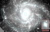 |
Fig. B.1. Spitzer IRAC 3.6 μm image showing the definition of our adopted environments. The inset on the bottom-right highlights the center with a different color stretch. |
All Tables
All Figures
|
Fig. 1. Molecular, atomic, and ionized gas in IC 342. This is a false-color composite of IC 342 showing molecular gas traced by our new NOEMA CO(1–0) survey (green), along with stellar light from DSS2 (white), atomic gas traced by the 21 cm line using the VLA (blue), and Hα emission from ionized gas (red). The dashed rectangle delimits the field of view observed with NOEMA and solid ellipses show galactocentric radii at 5, 10, 15, and 20 kpc. |
| In the text | |
|
Fig. 2. NOEMA survey of CO(1–0) emission from IC 342. The distribution of the CO(1–0) peak intensity at the native angular resolution (top left) and the intensity-weighted mean CO velocity at 90 pc resolution (top right) as revealed by our new CO survey. The images show spiral arms, abundant inter-arm emission, and a velocity field that mostly reflects a regularly rotating gas disk. The bottom panels show the molecular gas traced by CO in the context of atomic gas and stars. In these panels, the CO and H I data are shown at a common ∼350 pc resolution. The bottom left panel shows a map of the total neutral gas surface density adding molecular gas surface density to atomic gas surface density from Chiang et al. (2021). The white ellipses show 1, 2, 3 × Re and the gray dashed ellipse indicates 1 R25. The lower right panel shows the azimuthally averaged mass surface density profiles for atomic gas, molecular gas, and stellar mass estimated from the near-infrared. The stellar mass distribution using HST imaging is consistent with a nuclear star cluster and an exponential disk (Carson et al. 2015), while the presented profile suffers from the resolution of the WISE data. Our NOEMA survey covers the inner molecule-dominated region where the H I emission is depressed, including the CO-bright center. |
| In the text | |
|
Fig. 3. Giant molecular clouds or associations in IC 342. The top left panel shows the location of the molecular clouds that we catalog at 90 pc resolution. The size of each circle corresponds to the deconvolved radius and the color indicates which dynamical environment the cloud is assigned to (red shows interarm clouds, green arm cloud, and blue center clouds). The top right and bottom left panels show the cloud properties in σ2/R vs. Σmol space, in which clouds with a fixed virial parameter follow a diagonal line with a slope of unity in log–log space. Σmol is the average surface density within the FWHM size of each cloud, Σmol = MCO/(2πR2). We show the IC 342 clouds for each environment and clouds at the same resolution and sensitivity, but better velocity resolution, from PHANGS-ALMA (Rosolowsky et al. 2021, and Hughes et al., in prep.). The bottom left panel replaces individual clouds with running medians. The bottom right panel adopts a beam-wise approach in which each independent line of sight at a fixed 90 pc resolution supplies a measurement of line width and surface density (Sun et al. 2018, 2020b). Again we compare the IC 342 points to those from a large sample of PHANGS-ALMA galaxies and here we mark the channel width and approximate sensitivity limit for the IC 342 data with dashed lines (for a Gaussian CO line, FWHM = 2.35σ, so we always have more than one channel across the FWHM of the emission line). The bottom row also indicates the mass-weighted median (position of the color circles) and 16 − 84% range (span of the color horizontal or vertical line) for surface densities and line widths. These refer to the corresponding horizontal or vertical axis, with an arbitrary positioning along the perpendicular direction. The mass-weighted averages tend to lie at higher values than the bulk of the individual measurements because much of the molecular gas mass resides in a few high-mass clouds or associations. All panels tell a consistent story: arm clouds show mildly enhanced surface density and line width compared to inter-arm clouds, and the center shows significant enhancements in surface density and line width. The elevated line widths in the center indicate high virial parameters suggesting clouds with additional contributions to their line widths. The deviations from self-gravity virialization would be even more extreme if we adopted a CO-to-H2 conversion factor below the Galactic value used to construct these plots. The black crosses in the right panels show representative error bars for our measurements in IC 342, as explained in the main text. |
| In the text | |
|
Fig. 4. Star formation efficiency per gravitational free-fall time in 1.5 kpc regions. Each hexagonal point shows the integrated molecular gas depletion time for a 1.5 kpc diameter region as a function of the mass-weighted average τff (see Eq. (4)) for 90 pc resolution clouds in that region. A straight, diagonal line in this space, such as the dark red one, corresponds to a fixed ϵff, which could be expected if density variations represent the primary drivers of depletion time variations. We color the regions by galactocentric radius and calculate the implied ϵff for each region. We estimate a median ϵff of 0.45% with a 16 − 84% range of 0.33 − 0.71%, and we illustrate these with the solid red line and shaded pink region. For the central 1.5 kpc region, we illustrate the effect of switching from our adopted Galactic αCO to a starburst conversion factor. The black cross shows a representative error bar as explained in the main text. The plotted values can be found in Table A.3. |
| In the text | |
|
Fig. 5. Zooms of the molecular surface density, peak temperature, and line width towards the galaxy center. The images have been deprojected from the galaxy inclination on the plane of sky, and then converted to kpc using a distance of 3.45 Mpc. The yellow lines show our spiral mask, while the red and white ellipses delimit the extent of the bar and center environment, respectively (see Appendix B.3 for the definition of these environment). |
| In the text | |
|
Fig. B.1. Spitzer IRAC 3.6 μm image showing the definition of our adopted environments. The inset on the bottom-right highlights the center with a different color stretch. |
| In the text | |
Current usage metrics show cumulative count of Article Views (full-text article views including HTML views, PDF and ePub downloads, according to the available data) and Abstracts Views on Vision4Press platform.
Data correspond to usage on the plateform after 2015. The current usage metrics is available 48-96 hours after online publication and is updated daily on week days.
Initial download of the metrics may take a while.