| Issue |
A&A
Volume 679, November 2023
|
|
|---|---|---|
| Article Number | A146 | |
| Number of page(s) | 7 | |
| Section | Astrophysical processes | |
| DOI | https://doi.org/10.1051/0004-6361/202347455 | |
| Published online | 29 November 2023 | |
Plasma line detected by Voyager 1 in the interstellar medium: Tips and traps for quasi-thermal noise spectroscopy
1
LESIA, Observatoire de Paris, PSL Université, CNRS, Sorbonne Université, Université de Paris, 92195 Meudon, France
e-mail: This email address is being protected from spambots. You need JavaScript enabled to view it.
2
Dept. of Physics and Astronomy, University of Iowa, Iowa City, IA 52242, USA
Received:
13
July
2023
Accepted:
25
September
2023
Abstract
The quasi-thermal motion of plasma particles produces electrostatic fluctuations, whose voltage power spectrum induced on electric antennas reveals plasma properties. In weakly magnetised plasmas, the main feature of the spectrum is a line at the plasma frequency – proportional to the square root of the electron density – whose global shape can reveal the electron temperature, while the fine structure reveals the suprathermal electrons. Since it is based on electrostatic waves, quasi-thermal noise spectroscopy (QTN) provides in situ measurements. This method has been successfully used for more than four decades in a large variety of heliosphere environments. Very recently, it has been tentatively applied in the very local interstellar medium (VLISM) to interpret the weak line discovered on board Voyager 1 and in the context of the proposed interstellar probe mission. The present paper shows that the line is still observed in the Voyager Plasma Wave Science data, and concentrates on the main features that distinguish the plasma QTN in the VLISM from that in the heliosphere. We give several tools to interpret it in this medium and highlight the errors arising when it is interpreted without caution, as has recently been done in several publications. We show recent solar wind data, which confirm that the electric field of the QTN line in a weakly magnetised stable plasma is not aligned with the local magnetic field. We explain why the amplitude of the line does not depend on the concentration of suprathermal electrons, and why its observation with a short antenna does not require a kappa electron velocity distribution. Finally, we suggest an origin for the suprathermal electrons producing the QTN and we summarise the properties of the VLISM that could be deduced from an appropriate implementation of QTN spectroscopy on a suitably designed instrument.
Key words: plasmas / waves / instrumentation: miscellaneous / ISM: general
© The Authors 2023
 Open Access article, published by EDP Sciences, under the terms of the Creative Commons Attribution License (https://creativecommons.org/licenses/by/4.0), which permits unrestricted use, distribution, and reproduction in any medium, provided the original work is properly cited.
This article is published in open access under the Subscribe to Open model. This email address is being protected from spambots. You need JavaScript enabled to view it. to support open access publication.
1. Introduction
A weak continuous line close to the local plasma frequency fp has been discovered (Ocker et al. 2021) in spectra measured by the Voyager 1 Plasma Wave Science (PWS) instrument (Scarf & Gurnett 1977) in the very local interstellar medium (VLISM). Such a continuous line has been detected using long spectral averages and its weakness and stability suggest that it might possibly be produced by plasma quasi-thermal noise (QTN), despite the small antenna length of the PWS instrument.
The plasma QTN was discovered in the solar wind by Meyer-Vernet (1979) with the ISEE-3 radio receiver, which was then the most sensitive receiver ever flown (Knoll et al. 1978). This noise is due to the electrostatic field produced by the plasma particle quasi-thermal motion (Fejer & Kan 1969), detected by a sensitive wave receiver at the ports of an electric antenna. Since this electrostatic field is associated with the plasma velocity distributions (Sitenko 1967), in the case of stable distribution functions one can use QTN spectroscopy to reveal plasma properties such as the electron density and temperature (Meyer-Vernet & Perche 1989). This technique has been developed and used in a large variety of media in the heliosphere (Meyer-Vernet et al. 1998, 2017 and references therein), where the quasi-thermal noise is routinely observed with wave instruments and represents the long-wavelength limit for radioastronomy measurements from space (Meyer-Vernet et al. 2000). Because electrostatic waves are heavily damped, the QTN measurements are local, contrary to usual spectroscopy in astronomy. If the plasma is magnetised, then the spectrum has a complex structure including Bernstein waves, from which QTN spectroscopy reveals electron properties (Meyer-Vernet et al. 1993; Moncuquet et al. 1995; Schippers et al. 2013). If the plasma is weakly magnetised, as the interplanetary and interstellar media, then the QTN spectrum has a much simpler structure, with a line at the local plasma frequency fp produced by Langmuir waves. The density deduced from this line is recognised as a gold standard and used as a reference for calibrating other instruments.
Gurnett et al. (2021) proposed to interpret the fp line observed by the Voyager 1 PWS instrument in the VLISM as the QTN associated with an electron velocity distribution composed of the superposition of a cold Maxwellian at 7000 K and a ten times hotter kappa distribution with κ = 1.53; this proposed hot kappa distribution represented 50% of the density and therefore contributed considerably to the pressure. These authors also interpreted the absence of observations of the line before 2016 by arguing that the QTN electric field is oriented along the magnetic field B. They suggested that since the angle α between the Voyager antenna effective direction and B exceeded about 15°, the resulting weakening of the signal by the factor cos2α would hinder its observation.
These arguments have been contradicted by Meyer-Vernet et al. (2022), who showed in a short letter that the stable QTN electrostatic field near fp in the weakly magnetised VLISM should not be aligned with the static magnetic field. Therefore, its orientation could not be responsible for the absence of the line from Voyager 1 PWS measurements taken at locations near the heliopause. In addition to that, Meyer-Vernet et al. (2022) showed that a minute quantity of hot electrons with a power-law energy distribution is sufficient to explain the observations, since the amplitude of the line is independent of the proportion of these electrons provided they dominate the distribution at the high speeds producing the line (Chateau & Meyer-Vernet 1991; Meyer-Vernet et al. 2017). This property eliminated the need to assume a problematic kappa distribution. Nevertheless, in a recent review paper on the interstellar probe mission, Brandt et al. (2023) repeated the arguments that the detection of the QTN line at fp with a modest length antenna requires it to be nearly aligned with the ambient magnetic field and that the observed line can be interpreted with a kappa distribution with κ = 1.53.
In this context, the objective of the present study is two-fold: (i) explain how to perform QTN spectroscopy in the VLISM in order to avoid some previous mistakes and (ii) interpret the observed properties of the fp line identified on Voyager 1. The paper is structured as follows: Sect. 2 shows that the line continues to be observed in the available recent Voyager 1 PWS data, with a frequency consistent with Kurth et al. (2023), and summarises its properties; Sect. 3 presents recent solar wind measurements illustrating that the electric field of the stable QTN line in a weakly magnetised plasma is not aligned with the local magnetic field; Sect. 4 discusses the main differences between QTN spectroscopy in the heliosphere and in the VLISM, the traps to be avoided, and some useful tips; Sect. 5 suggests several explanations for the absence of the line close to the heliosheath and proposes an origin for the suprathermal electrons producing the observed fp line; and finally, we summarise the properties of the VLISM that could be derived with adequate instrumentation and implementation of QTN spectroscopy.
2. The Voyager QTN line
Figure 1 shows the weak continuous line near the local plasma frequency fp measured from the Voyager 1 PWS wideband data in the VLISM from early 2018 to late 2022. The line observed before late 2020 was published and discussed previously (Ocker et al. 2021; Burlaga et al. 2021; Gurnett et al. 2021; Richardson et al. 2022; Meyer-Vernet et al. 2022; Brandt et al. 2023). The two-year line continuation in 2021–2022 is consistent with the observations shown by Kurth et al. (2023).
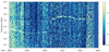 |
Fig. 1. Frequency–time spectrogram showing a portion of the weak continuous line previously published and its continuation from late 2020 until late 2022. The linear intensity scale is relative to the background level. The data from Voyager are available at https://pds.nasa.gov/. |
The spectrogram is built from fast Fourier transforms (FFT) of Voyager 1 PWS waveform data. These waveform data were designed to fit within an imaging subsystem (ISS) image frame. This frame is made of 800 lines, each filled up with 1600 4-bit waveform data at the 28.8 kHz sampling frequency, and is written in 48 s (including small data gaps between individual lines); for details, readers can refer to Kurth et al. (2023). All spectra used in the present analysis are the average of single FFT power spectra computed from each individual line. Because of a mismatch between the Deep Space Network and Voyager playback capabilities, only one out of every five of those 800 lines can be transmitted to Earth, making any enhancement of the spectral resolution by FFTing consecutive lines impossible. The best available spectral resolution of PWS wideband data is therefore limited to 28 800/1600 = 18 Hz – a limit that might be easily overcome in any future dedicated instrument. The noise equivalent bandwidth (NEBW) of the measurement is increased from 18 Hz to about 24 Hz because of the apodisation (Hamming window).
The measured line width is nearly 27 Hz, which is not significantly larger than the instrumental NEBW given the uncertainties. It follows that the line is not resolved, having a measured width close to the frequency resolution. This absence of resolution can be checked by comparing the observed line to the 2.4 kHz interference line, whose measured width appears similar despite its presumably quasi-Dirac shape (Fig. 2). So the intrinsic width of the fp line is expected to be smaller than (or equal to) 24 Hz. The figures were obtained using averages over a part (about 10 s) of the recorded 48 second data snapshots, spaced by 2.2 days or 7 days, depending on the available telemetry, without any detectable change in line width over the instrumental value.
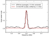 |
Fig. 2. Observed fp line (in black, linear scale) superimposed on the supply interference line (in red) scaled in amplitude and shifted in frequency. The fp line profile was obtained by averaging 45 300 good-quality spectra which were shifted to a common central frequency, fitted to a Gaussian profile, and acquired within the period shown in Fig. 1. The total power exceeds the background by about 20%, which means that the contribution of the line amounts to roughly 20% of the background. |
With a 7 days temporal resolution, the only notable event is a strong density increase of roughly 36% in 2020, with a rapid variation around May 2020 associated with a similar increase in magnetic field strength (Burlaga et al. 2021). This event took place unfortunately just after a data gap of about one month.
Over the 5 yr shown in Fig. 1 (from early 2018 to late 2022), the contribution of the QTN line amounts to about 20% of the background on average. This contribution is roughly two times higher than its mean value from September 2017 to late 2020 (Ocker et al. 2021; Meyer-Vernet et al. 2022), suggesting that the amplitude of the line increased, as shown in Fig. 3, where the line intensity is displayed as a function of its frequency. This increase, associated with the increase in density ( ), can be entirely attributed to the variation in the line intensity in proportion of
  in Eq. (6) (see Sect. 5). However, we note that the use of the automatic gain controlled (AGC) receiver and no telemetered information on the gain as well as in some cases extreme noise due to a low signal-to-noise ratio in the telemetry link makes this comparison somewhat uncertain.
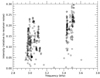 |
Fig. 3. Intensity of the line relative to the background as a function of its frequency, for the spectra acquired within the period shown in Fig. 1. The average power of the line of 14 ± 6% near 3 kHz increases to 20 ± 4% near 3.5 kHz, which is in agreement with Eq. (6). |
3. QTN fp line and magnetic field direction
As we noted in Sect. 1, Gurnett et al. (2021) and Brandt et al. (2023) have argued that the electric field of the QTN fp line is aligned with the ambient static magnetic field, in order to explain why the line was not detected on Voyager near the heliopause.
This argument is not expected to be correct in weakly magnetised stable plasmas, where the electron gyrofrequency fB = eB/(2πm) is negligible with respect to the plasma frequency. In the interstellar medium where the line is detected, fB/fp ∼ 4 × 10⁻³ (e.g., Burlaga et al. 2021). It follows that, with the values of the wave number k contributing to the line, the fB term is negligible in the equation of the generalised Langmuir mode (Willes & Cairns 2000)  , with θ being the angle between B and the longitudinal electric field (Meyer-Vernet et al. 2022). No variation in the QTN with the angle between the antenna direction and the magnetic field has ever been observed in weakly stable plasmas (Meyer-Vernet & Moncuquet 2020) during four decades of QTN observations, except a small variation due to the anisotropy of the electron temperature (Meyer-Vernet 1994).
Figure 4 shows a counter example of the claimed necessity for the antenna direction to be aligned with the local static magnetic field for measuring the QTN fp line in weakly magnetised plasmas. The top panel shows a spectrogram measured by the FIELDS instrument (Bale et al. 2016; Pulupa et al. 2017) in the solar wind during the 14th perihelion of Parker Solar Probe (PSP). In the bottom part of Fig. 4, panel a shows the spectral power at the fp peak, which is used on PSP to estimate the temperature of the suprathermal component of the electron velocity distribution (Moncuquet et al. 2020), panel b shows the electron density deduced from the spectra, panel c shows the ratio of the antenna length to the Debye length deduced as described in the paper cited above, and panel d shows the angle α between the antenna direction and the static magnetic field. With the ratio fB/fp ∼ (1 − 3)×10−2, the angle between the antenna direction and the magnetic field varies between 45 and 90° without affecting the amplitude of the QTN line, with a ratio between the antenna length L and the Debye length LD between 0.6 and 2.
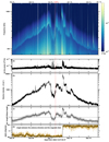 |
Fig. 4. Top panel: spectrogram acquired during the 14th PSP solar perihelion (closest solar distance 13.28 solar radii) with the FIELDS antenna, showing the plasma QTN, on which the fp line clearly emerges (cyan line varying between 90 kHz and 1 MHz). The heliocentric distance in solar radii is indicated at the top. Bottom panel: (a) spectral power at the peak, (b) total electron density, (c) ratio of the antenna length to the plasma Debye length, and (d) angle between the antenna direction and the magnetic field, showing a 180° variation at the heliospheric current sheet crossing (courtesy of FIELDS MAG). The superimposed black lines in panels c and d are one-hour rolling averages. The vertical dotted red line indicates the time of perihelion. The PSP spectrogram is available at https://research.ssl.berkeley.edu/data/psp/data/sci/fields/l2/rfs_lfr/2022/12/. |
4. Tips and traps for QTN spectroscopy in the interstellar medium
QTN measurements in the VLISM differ from those made currently in the heliosphere (Moncuquet et al. 2020) by several major aspects. First, the spatial scales are generally much larger in the VLISM (e.g., Fraternale et al. 2022; Richardson et al. 2023). So, the properties of the interstellar medium are generally much more constant in space and time (as seen from a spacecraft) than in the heliosphere. Furthermore, the high-frequency compressible turbulence has a much smaller amplitude (Ocker et al. 2021 and references therein). The resulting quasi-constancy of the electron density enables the spectra to be averaged for much longer times, so very weak features can be detected. For example, the Voyager interstellar line shown in Figs. 1 and 2 was detected by sampling the data over times that could be separated by one week, whereas the solar wind line shown in Fig. 4 was measured with an acquisition time ≃2 s by the Low Frequency Receiver of the FIELDS instrument on PSP (Pulupa et al. 2017). The QTN noise is indeed rarely integrated for more than a few seconds in the interplanetary medium because of the short-wavelength density fluctuations (Celnikier et al. 1987), which widen the fp line (Chateau & Meyer-Vernet 1991). This property enables one to detect the QTN line far below the instrumental noise of Voyager PWS, since the averaging increases the level of the signal to be detected compared to the fluctuations of the instrumental noise. The line measured in the interstellar medium does indeed have an average power of 10–20% of the receiver noise (Ocker et al. 2021; Meyer-Vernet et al. 2022). In contrast, the power spectral density in the PSP line shown in Fig. 4 is of the order of magnitude of 10−14 V2 Hz−1, which is higher than the instrumental noise (about 2.2 × 10⁻¹⁷ V2 Hz−1) by more than two orders of magnitude.
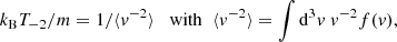
Second, the electron density is very small in the interstellar medium, which has two important consequences. The particle-free paths are very large. The Debye length is relatively large, exceeding the equivalent length of the Voyager antenna L ≃ 7.1 m (Gurnett et al. 2021). It is well known that in that case, the QTN fp line is minute in a Maxwellian plasma and still difficult to detect in the presence of a hot suprathermal Maxwellian component (Meyer-Vernet & Perche 1989). The Debye length
![Mathematical equation: $$ \begin{aligned} L_{\rm D} = [\epsilon _0 k_{\rm B} T_{-2}/(ne^2)]^{1/2} ,\end{aligned} $$](/articles/aa/full_html/2023/11/aa47455-23/aa47455-23-eq4.gif) (1)
(1)
where
 (2)
(2)
with f(v) being the electron 3D velocity distribution normalised to the electron density, is determined by the coldest electrons. Hence, when the distribution is composed of the superposition of a cold Maxwellian and a small proportion of suprathermal electrons, LD is determined by the temperature of the cold Maxwellian.
Third, although the shot noise is often a nuisance in the interplanetary medium, requiring the antennas to be very thin (Meyer-Vernet et al. 2017), the shot noise is expected to be very small in the interstellar medium because the photoelectron emission by the antenna is much smaller than the plasma electron current. This produces a negative antenna potential of a few times the electron energy, which strongly reduces the flux of incoming plasma electrons (Whipple 1981), and therefore the shot noise (Meyer-Vernet et al. 2017).
In general, a few theoretical properties of the QTN enable a simple measurement in weakly magnetised plasmas (Meyer-Vernet & Perche 1989; Meyer-Vernet et al. 2017), as the interplanetary and interstellar media. First, the plasma frequency reveals the electron density, provided the line emerges from the rest of the spectrum. And since the Langmuir wavelength tends to infinity at fp, the QTN measurement is equivalent to a detector of a large cross-section and is relatively immune to spacecraft perturbations (Meyer-Vernet et al. 1998).
Second, below the plasma frequency, the electron QTN spectrum is determined by electrons crossing a Debye length around the antenna. Each such electron induces a potential pulse of duration ∼1/(2πfp), producing a plateau below fp with an amplitude mainly depending on the cold component of the electron distribution. Although the level of this plateau can be calculated numerically (Meyer-Vernet & Perche 1989; Meyer-Vernet et al. 2017), an approximate measurement can be easily made via the following analytic formulas: L/LD ≪ 1: V2 ≃ [(2kBTm)1/2/(3π3/2ϵ0)](L/LD)2[1 + ln(LD/L)] ≃ 3.4 × 10⁻¹⁷T1/2(L/LD)2[1 + ln(LD/L)], 2 < L/LD < 7: V2 ≃ (kBTm)1/2/(π2ϵ0)≃4.1 × 10−17T1/2, and L/LD ≫ 1: V2 ≃ (π/2)1/2kBT/(ϵ0ωpL)≃3.5 × 10−14T/(n1/2L). Here, T is the electron temperature, m is the electron mass, and ωp = 2πfp. When the electron velocity distribution is the superposition of a cold Maxwellian and a hot dilute halo, the temperature in these formulas is roughly that of the cold component, as for the expression of the Debye length. For more complex distributions, detailed values are given by Meyer-Vernet et al. (2017). The above expressions neglect the contribution of the ions (Issautier et al. 1999).
Third, the high-frequency spectrum for (f/fp)(L/LD)≫1 is proportional to the electron total pressure: 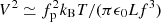 .
.
We now consider the fp peak. The Langmuir wave number at frequency f = fp + Δf with Δf/fp ≪ 1 is kL ≃ (ωp/vth)[2Δf/fp]1/2, where vth is the electron root-mean-square speed defined as
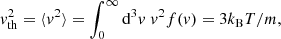 (3)
(3)
which also defines the temperature for velocity distributions that are not necessarily Maxwellian. The speed of the electrons producing the QTN at f = fp + Δf (with Δf/fp ≪ 1) is therefore
![Mathematical equation: $$ \begin{aligned} v_{\mathrm{ph} } \simeq \omega _{\rm p}/k_{\rm L} = v_{\mathrm{th} } [ f_{\rm p}/2\Delta f]^{1/2} .\end{aligned} $$](/articles/aa/full_html/2023/11/aa47455-23/aa47455-23-eq8.gif) (4)
(4)
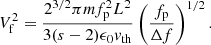
From Eqs. (3) and (4) with the assumed temperature T ≃ 7000°K (McComas et al. 2015), we deduce that the QTN at frequencies in the range fp < f < fp + δf, where fp ≃ 3.5 kHz and δf = 12 Hz is the maximum half-width of the line (Sect. 2), is produced by electrons with a speed faster than vph ≃ 6.8 × 10⁶ m s−1, which corresponds to energies above about 100 eV.
The QTN at frequency fp + Δf, where Δf/fp ≪ 1, measured with an antenna of length L, is given by (Meyer-Vernet et al. 2017)
![Mathematical equation: $$ \begin{aligned} V_{\rm f}^2 \simeq \frac{8 m v_{\rm ph} F(\omega _{\rm p}L/v_{\rm ph})}{\pi \epsilon _0 v_{\rm th}^2} \left[\frac{ \int _{v_{\rm ph}}^{\infty } \mathrm{d} v \; v \; f(v)}{ f(v_{\rm ph})} \right] ,\end{aligned} $$](/articles/aa/full_html/2023/11/aa47455-23/aa47455-23-eq9.gif) (5)
(5)
where vph is given by Eq. (4) and F(x) is the antenna response. Since ωpL/vph ≪ 1, we have F(x)≃x2/24 (Meyer-Vernet & Perche 1989).
The width of the line observed on Voyager is too small to be produced by a hot suprathermal Maxwellian (Meyer-Vernet et al. 2022), contrary to the QTN line generally observed in heliospheric plasmas. Such a thin line can be produced by a minute amount of hot electrons with a power-law energy distribution. Superimposing on a Maxwellian at temperature T, such a distribution fh(v)∝1/vs with s > 2 at energies exceeding ≃100 eV yields a distribution whose thermal speed vth is determined by the Maxwellian and whose value at v ≥ vph nearly equals fh(v). Therefore, the square bracket in Eq. (5) is determined by fh(v) and independent of the concentration of these electrons, and the QTN at frequency fp + Δf (with Δf/fp ≪ 1) is given by
 (6)
(6)
The power associated with frequencies closer to fp than Δf should be larger than this value in the absence of widening of the line by density fluctuations, but it cannot be measured at frequencies closer to fp than the frequency resolution, characterised by the instrumental NEBW. Hence the measured line width should be of the order of the frequency resolution, as observed. (We note that if the instrumental NEBW were much smaller, the speed of the electrons producing the peak would become relativistic.)
Approximating the peak level by the average of Eq. (6) between fp and fp + δf/2, corresponding to the half-width, and substituting fp ≃ 3.5 kHz, L ≃ 10/21/2 ≃ 7.1 m, T ≃ 7000°K, and s = 5, we obtain  V2 Hz−1. Adding the remaining QTN noise of the order of the plateau ≃10−15 V2 Hz−1 from the expressions written above, we get
  V2 Hz−1. With the published receiver noise of about 10−13 V2 Hz−1 (Kurth et al. 1979; Gurnett et al. 2021), the measured line shown in Fig. 2 has an average intrinsic level of the order of 2 × 10⁻¹⁴ V2 Hz−1, which is a few times larger than our theoretical estimate. However, the published receiver noise is based on the spectral density noise threshold of the spectrum analyser channels, whereas for the present work we used the waveform receiver, which could detect line emissions below this level with sufficient signal averaging, so the values of the theoretical and observed line levels are marginally compatible. We note that Eq. (6) shows that the intensity of the line would decrease if T or the instrumental NEBW were larger. We shall return to this point in Sect. 5.
We now evoke some traps into which one may fall when trying to apply QTN spectroscopy in the VLISM. The QTN calculations published by Gurnett et al. (2021) and Brandt et al. (2023) constitute interesting examples of these traps. We note that in Figs. 4 and 5 of the former paper, the plotted shot noise, which represents the main noise contribution below fp, is too large by factors of 10 and 20 for f < fp, respectively, even with a positive antenna potential as in the model by Meyer-Vernet & Perche (1989) cited in the caption of these figures. These errors may have arisen in particular because the antenna impedance should be calculated correctly in this frequency range (Zouganelis et al. 2009). A further little known trap is that the slope of the shot noise changes for f > fp, with a decrease much faster than 1/f2, because the rise time of the voltage pulses producing the shot noise is roughly the time for an electron to travel a Debye length. It follows that the squared Fourier transform decreases much more steeply than 1/f2 for f > fp (Meyer-Vernet 1985). Furthermore, with the expected small photoelectron emission from the antenna in the VLISM, the shot noise should become much smaller because of the expected negative antenna potential. In addition, the ion QTN (Issautier et al. 1999) is not negligible below fp with the parameters considered in the figure by Gurnett et al. (2021) reproduced by Brandt et al. (2023).
We now consider the proposed interpretation of the fp line by the superposition in equal proportions of a Maxwellian and a ten times hotter kappa distribution with κ = 1.53 (Fig. 7 by Gurnett et al. 2021, reproduced in Fig. 14 by Brandt et al. 2023). This highly publicised figure exhibits further traps.
As we already noted, the fp peak is determined by the suprathermal electrons, independently of their concentration. More precisely, the noise at frequencies between fp and fp + Δf is determined by the shape of the electron distribution at speeds exceeding the value given in Eq. (4). At such speeds, the contribution of the Maxwellian has considerably decreased, so the distribution assumed in these papers reduces to the kappa function, which itself reduces to a power law ∝1/vs with s = 2 × (κ + 1)≃5. Therefore, the QTN at frequency f = fp + Δf with the distribution assumed in these papers should be roughly equal to the value given in Eq. (6). However, as we already noted, the smaller the value of Δf, the higner the intensity, and the theoretical QTN should not be plotted closer to fp than the frequency resolution in order to compare it to the data. We note, finally, that such a figure showing a QTN peak level close to the receiver noise contradicts the observations, which show a much smaller value.
The caption of this figure is interesting, too, since it reveals a frequent misunderstanding of the QTN. The caption attributes the large level of the peak to the smallness of the Debye length of the kappa distribution. The origin of such a misunderstanding is that increasing the thermal speed vth indeed decreases the peak level and that the Debye length is proportional to vth if the plasma is Maxwellian. However, the small Debye length of a kappa distribution with a value of kappa close to 1.5 is produced by the small value of T−2 given by Eq. (2), which has no effect on the peak, independently of the problems raised by such a distribution (Meyer-Vernet et al. 2022).
5. Discussion and conclusion
If the absence of the stable fp line close to the heliopause does not come from the angle between the Voyager antenna direction and the magnetic field, we must find an alternative explanation. Meyer-Vernet et al. (2022) suggested that the density fluctuations, which do not prevent the detection of the line farther out, may increase close to the heliopause, where compressive fluctuations in the heliosheath are transmitted (Burlaga et al. 2015, 2018), without reaching large distances farther out (Zank et al. 2019). This may broaden the peak and therefore decrease its amplitude. This suggestion should be studied in detail, which is outside the scope of the present paper. Other possible explanations should be examined as well. First, the electron density is much smaller close to the heliopause, especially before 2015 (Kurth et al. 2023), which would decrease the intensity of the line according to Eq. (6). Second, this equation shows that the line intensity should decrease close to the heliopause if the electron temperature increases (e.g., Fraternale & Pogorelov 2021 and references therein) since the peak varies as the inverse of the thermal speed. In particular, if T ≃ 30 000 K or more as the ion temperature measured by Voyager 2 PLS immediately outside the heliopause, albeit with currents close to the instrument threshold (Richardson et al. 2019), the intensity of the line would decrease by a factor of two or more, as well as the QTN plateau. A third possibility is a variation in the energy spectrum of the suprathermal electrons and of their minimal energy which determines the intrinsic width of the line via Eq. (4).
On the other hand, as we noted in Sect. 2, the increase in line intensity in 2020 from 14% to 20% of the background when the frequency of the fp line increases from roughly 3 kHz–3.5 kHz (Fig. 3) is entirely attributable to this increase in the value of fp since Eq. (6) shows that the intensity of the line should be proportional to  .
.
An important question is: what is the origin of the suprathermal electrons of energy exceeding ∼100 eV assumed in the present paper in order to produce the QTN line? This energy is of the same order of magnitude as that of the electron beams suggested to produce the instability exciting the plasma oscillation events detected close to the heliopause (Gurnett et al. 2021).
We first note that the presence of suprathermal electrons near 100 eV is not surprising since with an ambient electron density of the order of 0.15 cm−3, their Coulomb-free path is much larger than the distance from the heliopause and other density gradients that might produce them.
We suggest below an original explanation for these suprathermal electrons: the presence of density gradients. In order to enforce plasma quasi-neutrality, density gradients produce ambipolar electric fields, of order of magnitude E given by the electron momentum equation, which can be approximated by eE ≃ kBT/H, where the scale height H is roughly given by H−1 ≃ n−1(dn/dx). Here, dn/dx is the space derivative of the density and the temperature gradient is neglected compared to that of the density in the electron momentum equation. If the electric field exceeds the Dreicer field ED given by eED ≃ 2kBT/lf (Dreicer 1959, 1960), with lf being the mean-free path of thermal electrons, electrons with an energy exceeding the thermal energy times 3ED/E may undergo runaway, yielding a non-thermal velocity distribution. Scudder (2019, 2023) suggested steady runaway as the origin of the ubiquitous suprathermal electrons in the solar wind and possibly other astrophysical contexts. Such a production of suprathermal electrons above about ∼100 times the thermal energy would thus require density gradients of scale height H ∼ 100 lf/6. With a Coulomb-free path of thermal electrons lf ≃ 0.15 AU in the LISM measured from Voyager 1’s available data, the required scale height would be a few AU if such a process acts in a steady way. This is similar to the scale height reported by Gurnett et al. (2013) and Kurth et al. (2023).
Finally, it is important to note that the available data make the analysis difficult. In addition to telemetry errors, observational gaps, and other problems, the very high instrumental noise requires long spectral averages to detect the line. Furthermore, the intrinsic power of the signal is unknown since the level of the automatic gain control was not telemetered, so the signal can only be deduced relative to the very large instrumental noise. With a modern sensitive instrument and antennas of 50 m length1, the QTN plateau enabling a simple measurement of the thermal electrons could be easily measured, as well as the plasma frequency peak, even in the absence of a significant suprathermal component. Measuring a suprathermal component with a power-law distribution for electrons of energy exceeding 100 eV as considered here requires an instrumental relative NEBW of the order of 3 × 10⁻³.
Further analysis should be performed to check the proposed mechanisms using future data from Voyager, which can bring new perspectives for the Interstellar Probe project.
See Interstellar Probe Concept Study Report at https://interstellarprobe.jhuapl.edu/.
Acknowledgments
W.S.K. acknowledges support by NASA through Contract 1622510 with the Jet Propulsion Laboratory and the use of the Space Physics Data Repository at the University of Iowa supported by the Roy J. Carver Charitable Trust.
References
- Bale, S. D., Goetz, K., Harvey, P. R., et al. 2016, Space Sci. Rev., 204, 49 [Google Scholar]
- Brandt, P. C., Provornikova, E., Bale, S. D., et al. 2023, Space Sci. Rev., 219, 18 [NASA ADS] [CrossRef] [Google Scholar]
- Burlaga, L. F., Florinski, V., & Ness, N. F. 2015, ApJ, 804, L31 [NASA ADS] [CrossRef] [Google Scholar]
- Burlaga, L. F., Florinski, V., & Ness, N. F. 2018, ApJ, 854, 20 [NASA ADS] [CrossRef] [Google Scholar]
- Burlaga, L. F., Kurth, W. S., Gurnett, D. A., et al. 2021, ApJ, 911, 61 [NASA ADS] [CrossRef] [Google Scholar]
- Celnikier, L. M., Muschietti, L., & Goldman, M. V. 1987, A&A, 181, 138 [NASA ADS] [Google Scholar]
- Chateau, Y. F., & Meyer-Vernet, N. 1991, J. Geophys. Res. Space Phys., 96, 5825 [CrossRef] [Google Scholar]
- Dreicer, H. 1959, Phys. Rev., 115, 238 [NASA ADS] [CrossRef] [Google Scholar]
- Dreicer, H. 1960, Phys. Rev., 117, 329 [NASA ADS] [CrossRef] [Google Scholar]
- Fejer, J. A., & Kan, J. R. 1969, Radio Sci., 4, 721 [NASA ADS] [CrossRef] [Google Scholar]
- Fraternale, F., & Pogorelov, N. V. 2021, ApJ, 906, 75 [NASA ADS] [CrossRef] [Google Scholar]
- Fraternale, F., Zhao, L., Pogorelov, N. V., et al. 2022, Front. Astron. Space Sci., 9, 353 [NASA ADS] [CrossRef] [Google Scholar]
- Gurnett, D. A., Kurth, W. S., Burlaga, L. F., et al. 2013, Science, 341, 1489 [NASA ADS] [CrossRef] [Google Scholar]
- Gurnett, D. A., Kurth, W. S., Burlaga, L. F., et al. 2021, ApJ, 921, 62 [NASA ADS] [CrossRef] [Google Scholar]
- Issautier, K., Meyer-Vernet, N., Moncuquet, M., et al. 1999, J. Geophys. Res. Space Phys., 104, 15665 [Google Scholar]
- Knoll, R., Epstein, G., Hoang, S., et al. 1978, IEEE Trans., 16, 199 [NASA ADS] [Google Scholar]
- Kurth, W. S., Gurnett, D. A., & Scarf, F. L. 1979, J. Geophys. Res. Space Phys., 84, 3413 [NASA ADS] [CrossRef] [Google Scholar]
- Kurth, W. S., Burlaga, L. F., Kim, T., et al. 2023, ApJ, 951, 71 [NASA ADS] [CrossRef] [Google Scholar]
- Lee, K. H., & Lee, L. C. 2019, Nat. Astron., 3, 154 [Google Scholar]
- McComas, D. J., Bzowski, M., Frisch, P., et al. 2015, ApJ, 801, 28 [NASA ADS] [CrossRef] [Google Scholar]
- Meyer-Vernet, N. 1979, J. Geophys. Res. Space Phys., 84, 5373 [CrossRef] [Google Scholar]
- Meyer-Vernet, N. 1985, Adv. Space Res., 5, 37 [NASA ADS] [CrossRef] [Google Scholar]
- Meyer-Vernet, N. 1994, Geophys. Res. Lett., 21, 397 [NASA ADS] [CrossRef] [Google Scholar]
- Meyer-Vernet, N., & Moncuquet, M. 2020, J. Geophys. Res. Space Phys., 125, e2019JA027723 [NASA ADS] [CrossRef] [Google Scholar]
- Meyer-Vernet, N., & Perche, C. 1989, J. Geophys. Res. Space Phys., 94, 2405 [NASA ADS] [CrossRef] [Google Scholar]
- Meyer-Vernet, N., Hoang, S., & Moncuquet, M. 1993, J. Geophys. Res. Space Phys., 98, 21163 [CrossRef] [Google Scholar]
- Meyer-Vernet, N., Hoang, S., Issautier, K., et al. 1998, in Measurement Techniques in Space Plasmas: Fields, GM 103, eds. R. Pfaff, J. E. Borovsky, & D. T. Young (Washington, DC: AGU), 205 [CrossRef] [Google Scholar]
- Meyer-Vernet, N., Hoang, S., Issautier, K., et al. 2000, in Astronomy at Long Wavelengths, GM 119, eds. R. G. Stone, & B. T. Tsurutani (Washington D.C.: AGU), 67 [CrossRef] [Google Scholar]
- Meyer-Vernet, N., Issautier, K., & Moncuquet, M. 2017, J. Geophys. Res. Space Phys., 122, 7925 [NASA ADS] [CrossRef] [Google Scholar]
- Meyer-Vernet, N., Lecacheux, A., Issautier, K., & Moncuquet, M. 2022, A&A, 658, L12 [NASA ADS] [CrossRef] [EDP Sciences] [Google Scholar]
- Moncuquet, M., Meyer-Vernet, N., & Hoang, S. 1995, J. Geophys. Res. Space Phys., 100, 21697 [NASA ADS] [CrossRef] [Google Scholar]
- Moncuquet, M., Meyer-Vernet, N., Issautier, K., et al. 2020, ApJS, 246, 44 [Google Scholar]
- Ocker, S. K., Cordes, J. M., Chatterjee, S., et al. 2021, Nat. Astron., 5, 761 [NASA ADS] [CrossRef] [Google Scholar]
- Pulupa, M., Bale, S. D., Bonnell, J. W., et al. 2017, J. Geophys. Res. Space Phys., 122, 2836 [Google Scholar]
- Richardson, J. D., Belcher, J. W., Garcia-Galindo, & Burlaga, L. F. 2019, Nat. Astron., 3, 1019 [NASA ADS] [CrossRef] [Google Scholar]
- Richardson, J. D., Burlaga, L. F., Elliott, H., et al. 2022, Space Sci. Rev., 218, 35 [NASA ADS] [CrossRef] [Google Scholar]
- Richardson, J. D., Bykov, A., Effenberger, F., et al. 2023, Space Sci. Rev., 219, 6 [NASA ADS] [CrossRef] [Google Scholar]
- Scarf, F. L., & Gurnett, D. A. 1977, Space Sci. Rev., 31, 289 [NASA ADS] [Google Scholar]
- Schippers, P., Moncuquet, M., Meyer-Vernet, N., et al. 2013, J. Geophys. Res. Space Phys., 118, 7170 [CrossRef] [Google Scholar]
- Scudder, J. D. 2019, ApJ, 885, 138 [Google Scholar]
- Scudder, J. D. 2023, ApJ, 944, 133 [NASA ADS] [CrossRef] [Google Scholar]
- Sitenko, A. G. 1967, Electromagnetic Fluctuations in Plasmas (New York: Academic Press) [Google Scholar]
- Whipple, E. C. 1981, Rep. Prog. Phys., 44, 1197 [NASA ADS] [CrossRef] [Google Scholar]
- Willes, A. J., & Cairns, I. H. 2000, Phys. Plasmas, 7, 3167 [NASA ADS] [CrossRef] [Google Scholar]
- Zank, G. P., Nakanotani, M., & Webb, G. M. 2019, ApJ, 887, 116 [NASA ADS] [CrossRef] [Google Scholar]
- Zouganelis, I., Maksimovic, M., Meyer-Vernet, N., et al. 2009, Radio Sci., 45, RS1005 [NASA ADS] [Google Scholar]
All Figures
|
Fig. 1. Frequency–time spectrogram showing a portion of the weak continuous line previously published and its continuation from late 2020 until late 2022. The linear intensity scale is relative to the background level. The data from Voyager are available at https://pds.nasa.gov/. |
| In the text | |
|
Fig. 2. Observed fp line (in black, linear scale) superimposed on the supply interference line (in red) scaled in amplitude and shifted in frequency. The fp line profile was obtained by averaging 45 300 good-quality spectra which were shifted to a common central frequency, fitted to a Gaussian profile, and acquired within the period shown in Fig. 1. The total power exceeds the background by about 20%, which means that the contribution of the line amounts to roughly 20% of the background. |
| In the text | |
|
Fig. 3. Intensity of the line relative to the background as a function of its frequency, for the spectra acquired within the period shown in Fig. 1. The average power of the line of 14 ± 6% near 3 kHz increases to 20 ± 4% near 3.5 kHz, which is in agreement with Eq. (6). |
| In the text | |
|
Fig. 4. Top panel: spectrogram acquired during the 14th PSP solar perihelion (closest solar distance 13.28 solar radii) with the FIELDS antenna, showing the plasma QTN, on which the fp line clearly emerges (cyan line varying between 90 kHz and 1 MHz). The heliocentric distance in solar radii is indicated at the top. Bottom panel: (a) spectral power at the peak, (b) total electron density, (c) ratio of the antenna length to the plasma Debye length, and (d) angle between the antenna direction and the magnetic field, showing a 180° variation at the heliospheric current sheet crossing (courtesy of FIELDS MAG). The superimposed black lines in panels c and d are one-hour rolling averages. The vertical dotted red line indicates the time of perihelion. The PSP spectrogram is available at https://research.ssl.berkeley.edu/data/psp/data/sci/fields/l2/rfs_lfr/2022/12/. |
| In the text | |
Current usage metrics show cumulative count of Article Views (full-text article views including HTML views, PDF and ePub downloads, according to the available data) and Abstracts Views on Vision4Press platform.
Data correspond to usage on the plateform after 2015. The current usage metrics is available 48-96 hours after online publication and is updated daily on week days.
Initial download of the metrics may take a while.