| Issue |
A&A
Volume 658, February 2022
|
|
|---|---|---|
| Article Number | L12 | |
| Number of page(s) | 5 | |
| Section | Letters to the Editor | |
| DOI | https://doi.org/10.1051/0004-6361/202243030 | |
| Published online | 23 February 2022 | |
Letter to the Editor
Weak line discovered by Voyager 1 in the interstellar medium: Quasi-thermal noise produced by very few fast electrons
LESIA, Observatoire de Paris, PSL Université, CNRS, Sorbonne Université, Université de Paris, 92195 Meudon, France
e-mail: This email address is being protected from spambots. You need JavaScript enabled to view it.
, This email address is being protected from spambots. You need JavaScript enabled to view it.
, This email address is being protected from spambots. You need JavaScript enabled to view it.
Received:
3
January
2022
Accepted:
8
February
2022
Abstract
A weak continuous line has been recently discovered onboard Voyager 1 in the interstellar medium, whose origin raised two major questions. First, how can this line be produced by plasma quasi-thermal noise on the Voyager short antenna? Second, why does this line emerge at some distance from the heliopause? We provide a simple answer to these questions, which elucidates the origin of this line. First, a minute quantity of supra-thermal electrons, as generally present in plasmas – whence the qualifier ‘quasi-thermal’ – can produce a small plasma frequency peak on a short antenna, of amplitude independent of the concentration of these electrons; furthermore, the detection required long spectral averages, alleviating the smallness of the peak compared to the background. We therefore attribute the observed line to a minute proportion of fast electrons that contribute negligibly to the pressure. Second, we suggest that, up to some distance from the heliopause, the large compressive fluctuations ubiquitous in this region prevent the line to emerge from the statistical fluctuations of the receiver noise because it is blurred out by the averaging required for detection, especially in the presence of short-wavelength density fluctuations. These results open up novel perspectives for interstellar missions, by showing that a minute proportion of fast electrons may be sufficient to measure the density even with a relatively short antenna, because the quietness of the medium enables a large number of spectra to be averaged.
Key words: plasmas / methods: observational / ISM: general / radio continuum: ISM
© N. Meyer-Vernet et al. 2022
 Open Access article, published by EDP Sciences, under the terms of the Creative Commons Attribution License (https://creativecommons.org/licenses/by/4.0), which permits unrestricted use, distribution, and reproduction in any medium, provided the original work is properly cited.
1. Introduction
Ocker et al. (2021) (see also Burlaga et al. 2021) have recently discovered a weak continuous line close to the local plasma frequency on the Voyager 1 Plasma Wave System (PWS) instrument (Scarf & Gurnett 1977) in the interstellar medium. The origin of this line was not understood since a plasma quasi-thermal noise (QTN) origin was deemed problematic.
The plasma QTN is produced by the quasi-thermal motion of ambient plasma electrons, which induce electric fluctuations (Sitenko 1967) detected in situ by electric antennas. At frequencies below the plasma frequency fp, the electrons are Debye shielded, so their thermal motion produces voltage pulses shorter than the inverse frequency of observation, yielding a spectral plateau. Above fp, the quasi-thermal motions excite Langmuir waves, producing a spectral peak near fp as well as a power spectrum proportional to the electron pressure at high frequencies (Meyer-Vernet & Perche 1989). Since the discovery of this noise in the interplanetary medium (Meyer-Vernet 1979; Couturier et al. 1981), calculations of it have been extended to flat-top (Chateau & Meyer-Vernet 1989) and Kappa velocity distributions (Chateau & Meyer-Vernet 1991; Zouganelis 2008; Le Chat et al. 2009), to magnetised plasmas (Sentman 1982; Meyer-Vernet et al. 1993), and to include ions (Issautier et al. 1999). Spectroscopy of this noise has been used to measure in situ the electron density and temperature and the properties of supra-thermal electrons in the solar wind as well as in planetary and cometary environments on the spacecraft ISEE3-ICE, Ulysses, WIND, Cassini (Meyer-Vernet et al. 2017, and references therein), and more recently, Parker Solar Probe (PSP; Moncuquet et al. 2020).
Since the Langmuir wave phase speed exceeds the electron thermal speed by a larger and larger margin as the frequency approaches fp, whereas electric antennas are mainly sensitive to wavelengths of the order of their length, the peak appears only on antennas longer than the Debye length if the plasma is Maxwellian. However, because of the strong increase in the wave phase speed close to fp, the presence of supra-thermal electrons of similar speed produces a peak that still exists for antennas shorter than the Debye length, albeit with a smaller amplitude (Meyer-Vernet & Perche 1989; Chateau & Meyer-Vernet 1991). Figure 1 shows such an example where the line appears clearly on the 2 m antenna of the PSP FIELDS instrument (Bale et al. 2016), even when the Debye length estimated via QTN spectroscopy (bottom panel) exceeds the equivalent antenna length. This line amounts to about 0.5 × 10⁻¹⁴ V2 Hz−1 at the receiver ports (Fig. 1), which corresponds to about 6 × 10⁻¹⁴ V2 Hz−1 at the antenna ports (considering the gain factor); it was interpreted as QTN produced by a few percent of supra-thermal electrons of temperature of the order of 100 eV (Moncuquet et al. 2020).
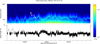 |
Fig. 1. Spectrogram acquired during the third PSP solar perihelion (August–September 2019) with the FIELDS antenna, showing the plasma QTN on which the fp line emerges clearly (cyan line). The plasma Debye length is plotted in black in the bottom panel. |
Therefore, a fp line can be observed in the presence of a small proportion of supra-thermal electrons, even with a relatively short antenna, if the radio receiver is sensitive enough (as is the case for the PSP/FIELDS instrument) or if the plasma frequency is sufficiently constant to enable it to emerge when a large number of spectra are averaged (as is the case of the Voyager/PWS instrument, as we will show in the next section). In the interplanetary medium, such averaging cannot be performed because of the perturbations and the ubiquitous short-wavelength density fluctuations (Celnikier et al. 1987).
A crucial property of the peak is that its height only depends on the velocity profile at speeds close to the wave phase speed at the measuring frequency (Chateau & Meyer-Vernet 1991; Meyer-Vernet et al. 2017). In other words, the height of the peak depends on the energy of supra-thermal electrons, not on their concentration; in contrast, increasing this concentration tends to increase the peak width. Hence, to explain the observed Voyager thin line, it is not necessary to assume 50% supra-thermals, which increases the pressure by a large factor, as Gurnett et al. (2021) did.
2. QTN in the quiet local interstellar medium
The Langmuir wave number responsible for the line at frequency f = fp + Δf with Δf/fp ≪ 1 is
![Mathematical equation: $$ \begin{aligned} k_{\rm L} = (\omega _{\rm p}/{ v}_{\mathrm{th} }) [2 \Delta f/f_{\rm p}]^{1/2}, \end{aligned} $$](/articles/aa/full_html/2022/02/aa43030-22/aa43030-22-eq1.gif) (1)
(1)
where ωp = 2πfp and
 (2)
(2)
Here vth is the electron mean square speed, T the temperature, f(v) the electron 3D-velocity distribution, and m the electron mass. The phase speed producing the QTN near fp is therefore
![Mathematical equation: $$ \begin{aligned} { v}_{\mathrm{ph} } \simeq \omega _{\rm p}/k_{\rm L} = { v}_{\mathrm{th} } [f_{\rm p}/2\Delta f]^{1/2}. \end{aligned} $$](/articles/aa/full_html/2022/02/aa43030-22/aa43030-22-eq3.gif) (3)
(3)
Ocker et al. (2021) indicate a frequency resolution of about δf ≃ 10 Hz, of the same order of magnitude as the line width. This corresponds to Δf/fp ≃ 3 × 10⁻³, so Eq. (3) yields the wave phase speed vph ≃ 7 × 10⁶ m s−1 at frequency fp + δf, for T = 7000 K. The electrons producing the QTN peak are thus expected to have an energy of the order of 100 eV or larger. We note that the relative velocity v between the plasma and the spacecraft, which yields a relative Doppler-shift v/vph ≃ 0.5%, might modify the shape of the line with this frequency resolution.
The QTN peak at the ports of an antenna of length L is given by (Meyer-Vernet et al. 2017)
![Mathematical equation: $$ \begin{aligned} V_{\rm f}^2 \simeq \frac{8 m { v}_{\mathrm{ph} } F(\omega _{\rm p}L/{ v}_{\mathrm{ph} })}{\pi \epsilon _0 { v}_{\mathrm{th} }^2} \left[\frac{\int _{{ v}_{\mathrm{ph} }}^{\infty }\mathrm{d}{ v} \; { v} \; f({ v})}{f({ v}_{\mathrm{ph} })}\right], \end{aligned} $$](/articles/aa/full_html/2022/02/aa43030-22/aa43030-22-eq4.gif) (4)
(4)
where vph is given by (3) and F(x) is the antenna response, given for ωpL/vph ≪ 1, by
 (5)
(5)
We first estimate the QTN peak by superimposing on the local interstellar medium (LISM) velocity distribution (assumed to be a Maxwellian of density n = 0.11 cm−3 and temperature T = 7000 K) a minute proportion nh/n ≪ 1 of Maxwellian electrons of temperature Th ≫ T, namely  . We see below that to produce a small enough line width, nh should be so minute that it does not significantly change the temperature T (or the pressure).
A sufficiently large ratio Th/T can produce a high peak, but for L/LD < 1 the peak width is set by the frequency at which the hot Maxwellian contributes to roughly half of the distribution at the corresponding phase speed (Meyer-Vernet & Perche 1989; Meyer-Vernet et al. 2017), that is,
 (6)
(6)
Using Eqs. (2) and (3), we deduce the relative width of the peak as
![Mathematical equation: $$ \begin{aligned} \Delta f/f \simeq (3/4)/\ln [n T_{\rm h}^{3/2}/(n_{\rm h} T^{3/2})]. \end{aligned} $$](/articles/aa/full_html/2022/02/aa43030-22/aa43030-22-eq8.gif) (7)
(7)
Such a width, depending in a logarithmic way on the concentration of supra-thermals, is difficult to reconcile with the very thin observed line, unless an infinitesimal proportion of supra-thermal electrons is assumed.
Therefore, we instead superimpose on the LISM Maxwellian a minute proportion of electrons with a power-law distribution fh(v) ∝ 1/vs (with s > 2) at speeds above vmin, in a speed range that includes the phase speeds producing the line and a few times these speeds and with a density that ensures that the power law exceeds the Maxwellian at these speeds. Because vph/vth ≫ 1, the Maxwellian has decreased by a huge factor at such speeds. Hence, the supra-thermal electrons largely dominate the total distribution at the speeds that produce the line, even if they contribute negligibly to the electron density and temperature or pressure. We note that the frequency resolution ensures that vph ≪ c (the velocity of light in vacuum).
With such supra-thermal electrons, the whole distribution in Eq. (4) can be replaced by f(v)∝1/vs at speeds v ≥ vph, and so the bracket equals  . Therefore, Eqs. (3)–(5) yield at frequency fp + Δf
 (8)
(8)
if vph ≥ vmin, which implies from Eq. (3)
 (9)
(9)
Approximating the peak level at frequency resolution δf by the average, ![Mathematical equation: $ {\propto}[\int_{f_{\rm p}}^{f_{\rm p} + \delta f} {\rm d}f/(f-f_{\rm p})^{1/2}]/\delta f = 2/\delta f^{1/2} $](/articles/aa/full_html/2022/02/aa43030-22/aa43030-22-eq12.gif) , we get at the antenna ports
, we get at the antenna ports
 (10)
(10)
if the relative frequency resolution δf/fp is smaller than the limit given by Eq. (9); with δf ≃ 10 Hz, this requires a minimum energy of supra-thermals of about 100 eV. Level (10) represents the QTN Langmuir wave contribution, to which, since L < LD, one must add the remaining contribution of the order of the plateau level, which is roughly equal to 10−15 V2 Hz−1 for these parameters (Meyer-Vernet & Perche 1989). Since kLL ≪ 1, we substitute  for the Voyager V antennas, as an approximation (Meyer-Vernet & Moncuquet 2020). Thus Eq. (10) yields
  V2 Hz−1.
If s = 5 − 7, which corresponds to a differential flux of dJ/dE ∝ E−p with p = 1.5 − 2.5 for sub-relativistic particles, we get  V2 Hz−1. A roughly twice larger spectral resolution, as shown in Figs. 3 and 4, would change these values by a factor of
  , and the minimum energy of supra-thermals by a factor of 2. Given the approximations used, we estimate these levels to be accurate within a factor of 3.
Since level (10) is proportional to the square root of the inverse of the relative frequency resolution, the line width will be of the same order of magnitude as the frequency resolution if it is not widened by the density variations during the time of integration.
This is illustrated in Fig. 2 which shows the fp line calculated with a frequency resolution δf/f ≃ 10−3 for Kappa distributions κ = 2 and 1.7, respectively (Le Chat et al. 2009). Such distributions are convenient for numerically estimating the peak because at frequencies sufficiently close to fp, the phase speed vph is so large that (i) a minute proportion of Kappa-distributed supra-thermals dominates the whole velocity distribution at vph and (ii) the Kappa itself reduces to a power law with s = 2(κ + 1). Contrary to Gurnett et al. (2021), we did not consider smaller values of κ, which would give rise to convergence problems, needing to be regularised (Scherer et al. 2018).
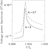 |
Fig. 2. QTN fp peak produced by Kappa distributions, with a relative frequency resolution δf/fp ≃ 10−3. As explained in the text, such distributions are convenient computational tools for estimating the peak produced by superimposing on a Maxwellian a minute proportion of power-law-distributed electrons of speeds exceeding the wave phase speed. |
Figure 2 also illustrates that, contrary to a common misunderstanding (Gurnett et al. 2021), the decrease in Debye length as κ decreases does not significantly increase the Langmuir wave contribution to the QTN (even though it changes somewhat the other contribution that depends on low-energy electrons) (Chateau & Meyer-Vernet 1991). This is because kL does not depend on (1/⟨v−2⟩)1/2, which determines LD, but on vth = ⟨v2⟩1/2; only for Maxwellians are both quantities proportional.
The measured amplitude cannot be calibrated because the gain values of the automatic gain control were not re-transmitted to the ground. However, the total average intensity can be compared to that of the background. Figure 3 shows such an example obtained when the line visibility is not ambiguous (i.e. after September 2017, see Fig. 4) by averaging spectra over about 2600 s distributed over 2.5 years in order to reduce the statistical fluctuations of the steady background level and make the line emerge. One sees that the contribution of the line to the total intensity is smaller than the background by roughly one order of magnitude on average, and its width is not significantly different from the achievable spectral resolution, given the expected broadening due to the uncertainty in frequency location and the expected intensity variations of the line over time. This weak line level confirms the results of Ocker et al. (2021) and contradicts the interpretation by Gurnett et al. (2021) that the QTN should exceed the receiver noise.
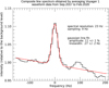 |
Fig. 3. Line profile (linear scale) obtained by averaging 42 600 spectra shifted to a common central frequency by fitting a Gaussian profile (in red). The total intensity exceeds the background by 11%, which means that the contribution of the line is smaller than the background level by about one order of magnitude and that the line width is not significantly different from the spectral resolution. |
With the published receiver noise (Kurth et al. 1979; Gurnett et al. 2021), this yields an average measured level of the order of 10−14 V2 Hz−1, which is marginally compatible with our estimates. However, the receiver noise is very probably overestimated below 20 kHz, since the published values are close to the sum of the quasi-thermal and the shot noise at the beginning of the Voyager mission. Hence the minimum measured level at these frequencies was not set by the receiver noise, but by the QTN, which represents a radio background (Meyer-Vernet 2000) unrecognised at this epoch. Furthermore, the published receiver noise was deduced by multiplying by the square of the equivalent antenna length for electromagnetic waves, which has since been revaluated to a smaller value (Meyer-Vernet et al. 1996).
Therefore, our result is expected to explain the observed line, both in terms of amplitude and width.
3. Emergence of the line at several AU from the heliopause
It has been suggested that the lack of observation of the line close to the heliopause is due to the QTN decrease by the factor cos2θ where θ is the angle between the antenna effective axis and the magnetic field B (Gurnett et al. 2021). However, this interpretation would require that the electric field be aligned with B, which is doubtful because of the smallness of B and because of the frequency resolution. Indeed, the electric field is instead perpendicular to B at the upper-hybrid frequency  , where fB = eB/(2πm) is the electron gyrofrequency (Stix 1962). Since fB/fp = 3.7 × 10⁻³, fUH differs from fp by less than 10−5 fp, which is much less than the frequency resolution. In other words, the QTN line is not expected to be affected by the magnetic field. This can also be understood from the dispersion equation of the generalised Langmuir mode (Willes & Cairns 2000)
  , θ being the angle between B and the longitudinal electric field, since the fB term is negligible.
We suggest instead that the detection of the line is impeded when density fluctuations alter its frequency, fp, too much during the time of integration required to detect the line. These fluctuations broaden the peak in relative value by one-half of the relative density fluctuations and decrease its height by roughly the ratio of the original peak width to the broadened value. This is the reason why one does not integrate the QTN noise over timescales exceeding a few seconds in the interplanetary medium, where perturbations and short-wavelength density fluctuations are ubiquitous (Chateau & Meyer-Vernet 1991).
Given the velocity of Voyager 1 (about 17 km s−1 in 2020) and PWS sampling occurring every two days at best, the medium was probed at points several millions of kilometres apart. In the quiet interstellar medium where the fp line is detected, the density fluctuations are so small that the frequency of the fp line changes very weakly, and is not blurred out after averaging. The value Δn/n = 0.034 found by Ocker et al. (2021) was derived by integrating the fluctuation spectrum up to the larger observed fluctuation scale of 10 AU, which corresponds to 2.8 years. A sufficiently small time of integration would broaden the line by less than the frequency resolution. However, the density fluctuations are expected to be higher closer to the heliopause, where compressive fluctuations in the heliosheath are transmitted across the heliopause (Burlaga et al. 2015, 2018), but they are not expected to reach large distances farther out (Zank et al. 2019). Depending on their amplitude and spectrum at scales corresponding to the time of integration, the line may be blurred out, especially if the short-wavelength turbulence, including the enhanced turbulence at kinetic scales (Lee & Lee 2019) is important. Conversely, the disappearance of the line for a given time of integration might be used to deduce the amplitude of the density fluctuations. We also note that the numerous solar-wind-initiated perturbations in this region producing intense emissions (see Fig. 4) impede long-term averages, and the large-scale variations in density compromise the localisation of the line necessary to detect it.
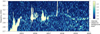 |
Fig. 4. Spectrogram of the interstellar line, built from Voyager 1 PWS waveform data with a spectral resolution of 23 Hz (using Fourier transforms of 1600 waveform samples, clocked at 28.8 kHz and Hamming-windowed). |
4. Discussion and conclusion
We have shown that superimposing a minute quantity of electrons with a hard power-law velocity distribution above about 100 eV on the LISM Maxwellian at 7000 K produces a QTN peak that explains the observed line. The width is of the order of the frequency resolution if the density fluctuations during the time of integration do not broaden the line, and the amplitude explains the observations, even better if the receiver noise level is a little lower than what has been published.
As in many dilute plasmas, the presence of supra-thermal electrons is not surprising (Scudder 2019), since the Coulomb free path increases as the energy squared. With an ambient electron density of the order of n ≃ 0.1 cm−3, the Coulomb free path of electrons of energy E ≃ 100 eV is about  AU. This is very large compared to the relevant scales and to distances from shocks that may produce such electrons and to distances from the heliopause. Several other equilibrium processes are operating (Draine & Kreisch 2018), but they concern smaller energies.
Since the region close to the heliopause is filled with compressive fluctuations from the heliosheath that do not penetrate very far into the quiet interstellar medium, we suggest that the corresponding density fluctuations may blur out the line there, especially if the short-wavelength turbulence is important, whereas these fluctuations have sufficiently decreased farther out to have only a small effect. Furthermore, the long-term variations in density may compromise the localisation of the line required in the detection process. More detailed comparisons of the QTN theory with the observations with different averaging at different epochs could reveal more properties of the medium.
The present calculations do not consider the contribution of cosmic rays to the QTN, which takes place much closer to fp than the frequency resolution. However, it might be interesting to generalise the calculations to relativistic speeds, in order to estimate this contribution.
Our results provide new perspectives for interstellar probes, showing for the first time that, thanks to the quietness of the medium, a minute proportion of supra-thermal electrons may be sufficient to enable the electron density to be measured with antennas shorter than the Debye length, even though long antennas are mandatory for accurately measuring the electron temperature.
References
- Bale, S. D., Goetz, K., Harvey, P. R., et al. 2016, Space Sci. Rev., 204, 49 [Google Scholar]
- Burlaga, L. F., Florinski, V., & Ness, N. F. 2015, ApJ, 804, L31 [NASA ADS] [CrossRef] [Google Scholar]
- Burlaga, L. F., Florinski, V., & Ness, N. F. 2018, ApJ, 854, 20 [NASA ADS] [CrossRef] [Google Scholar]
- Burlaga, L. F., Kurth, W. S., Gurnett, D. A., et al. 2021, ApJ, 911, 61 [NASA ADS] [CrossRef] [Google Scholar]
- Celnikier, L. M., Muschietti, L., & Goldman, M. V. 1987, A&A, 181, 138 [NASA ADS] [Google Scholar]
- Chateau, Y. F., & Meyer-Vernet, N. 1989, J. Geophys. Res.: Space Phys., 94, 15407 [NASA ADS] [CrossRef] [Google Scholar]
- Chateau, Y. F., & Meyer-Vernet, N. 1991, J. Geophys. Res., 96, 5825 [NASA ADS] [CrossRef] [Google Scholar]
- Couturier, P., Hoang, S., Meyer-Vernet, N., & Steinberg, J.-L. 1981, J. Geophys. Res.: Space Phys., 86, 11127 [NASA ADS] [CrossRef] [Google Scholar]
- Draine, B. T., & Kreisch, C. D. 2018, ApJ, 262, 30 [NASA ADS] [CrossRef] [Google Scholar]
- Gurnett, D. A., Kurth, W. S., Burlaga, L. F., et al. 2021, ApJ, 921, 62 [NASA ADS] [CrossRef] [Google Scholar]
- Issautier, K., Meyer-Vernet, N., Moncuquet, M., et al. 1999, J. Geophys. Res., 104, 15665 [Google Scholar]
- Kurth, W. S., Gurnett, D. A., & Scarf, F. L. 1979, J. Geophys. Res.: Space Phys., 84, 3413 [NASA ADS] [CrossRef] [Google Scholar]
- Le Chat, G., Issautier, K., Meyer-Vernet, N., et al. 2009, Phys. Plasmas, 16, 102903 [CrossRef] [Google Scholar]
- Lee, K. H., & Lee, L. C. 2019, Nat. Astron., 3, 154 [Google Scholar]
- Meyer-Vernet, N. 1979, J. Geophys. Res.: Space Phys., 84, 5373 [NASA ADS] [CrossRef] [Google Scholar]
- Meyer-Vernet, N. 2000, in Astronomy at Long Wavelengths, ed. R. G. Stone, 67 [Google Scholar]
- Meyer-Vernet, N., & Moncuquet, M. 2020, J. Geophys. Res.: Space Phys., 125, A027723 [Google Scholar]
- Meyer-Vernet, N., & Perche, C. 1989, J. Geophys. Res.: Space Phys., 94, 2405 [NASA ADS] [CrossRef] [Google Scholar]
- Meyer-Vernet, N., Hoang, S., & Moncuquet, M. 1993, J. Geophys. Res.: Space Phys., 98, 21163 [NASA ADS] [CrossRef] [Google Scholar]
- Meyer-Vernet, N., Lecacheux, A., & Pedersen, B. M. 1996, Icarus, 123, 113 [NASA ADS] [CrossRef] [Google Scholar]
- Meyer-Vernet, N., Issautier, K., & Moncuquet, M. 2017, J. Geophys. Res.: Space Phys., 122, 7925 [NASA ADS] [CrossRef] [Google Scholar]
- Moncuquet, M., Meyer-Vernet, N., Issautier, K., et al. 2020, ApJS, 246, 44 [Google Scholar]
- Ocker, S. K., Cordes, J. M., Chatterjee, S., et al. 2021, Nat. Astron., 5, 761 [NASA ADS] [CrossRef] [Google Scholar]
- Scarf, F. L., & Gurnett, D. A. 1977, Space Sci. Rev., 31, 289 [NASA ADS] [Google Scholar]
- Scherer, K., Fichtner, H., & Lazar, M. 2018, Eur. Lett., 120, 50002 [Google Scholar]
- Scudder, J. D. 2019, ApJ, 885, 138 [Google Scholar]
- Sentman, D. D. 1982, J. Geophys. Res.: Space Phys., 87, 1455 [NASA ADS] [CrossRef] [Google Scholar]
- Sitenko, A. G. 1967, Electromagnetic Fluctuations in Plasmas (New York: Academic Press) [Google Scholar]
- Stix, T. H. 1962, The Theory of Plasma Waves (London: McGraw-Hill), 223 [Google Scholar]
- Willes, A. J., & Cairns, I. H. 2000, Phys. Plasmas, 7, 3167 [NASA ADS] [CrossRef] [Google Scholar]
- Zank, G. P., Nakanotani, M., & Webb, G. M. 2019, ApJ, 887, 116 [NASA ADS] [CrossRef] [Google Scholar]
- Zouganelis, I. 2008, J. Geophys. Res.: Space Phys., 113, A0111 [Google Scholar]
All Figures
|
Fig. 1. Spectrogram acquired during the third PSP solar perihelion (August–September 2019) with the FIELDS antenna, showing the plasma QTN on which the fp line emerges clearly (cyan line). The plasma Debye length is plotted in black in the bottom panel. |
| In the text | |
|
Fig. 2. QTN fp peak produced by Kappa distributions, with a relative frequency resolution δf/fp ≃ 10−3. As explained in the text, such distributions are convenient computational tools for estimating the peak produced by superimposing on a Maxwellian a minute proportion of power-law-distributed electrons of speeds exceeding the wave phase speed. |
| In the text | |
|
Fig. 3. Line profile (linear scale) obtained by averaging 42 600 spectra shifted to a common central frequency by fitting a Gaussian profile (in red). The total intensity exceeds the background by 11%, which means that the contribution of the line is smaller than the background level by about one order of magnitude and that the line width is not significantly different from the spectral resolution. |
| In the text | |
|
Fig. 4. Spectrogram of the interstellar line, built from Voyager 1 PWS waveform data with a spectral resolution of 23 Hz (using Fourier transforms of 1600 waveform samples, clocked at 28.8 kHz and Hamming-windowed). |
| In the text | |
Current usage metrics show cumulative count of Article Views (full-text article views including HTML views, PDF and ePub downloads, according to the available data) and Abstracts Views on Vision4Press platform.
Data correspond to usage on the plateform after 2015. The current usage metrics is available 48-96 hours after online publication and is updated daily on week days.
Initial download of the metrics may take a while.