| Issue |
A&A
Volume 679, November 2023
|
|
|---|---|---|
| Article Number | A96 | |
| Number of page(s) | 18 | |
| Section | Cosmology (including clusters of galaxies) | |
| DOI | https://doi.org/10.1051/0004-6361/202346992 | |
| Published online | 15 November 2023 | |
A new measurement of the expansion history of the Universe at z = 1.26 with cosmic chronometers in VANDELS
1
Dipartimento di Fisica e Astronomia “Augusto Righi”–Università di Bologna, Via Piero Gobetti 93/2, 40129 Bologna, Italy
e-mail: elena.tomasetti2@unibo.it
2
INAF – Osservatorio di Astrofisica e Scienza dello Spazio di Bologna, Via Piero Gobetti 93/3, 40129 Bologna, Italy
3
Institute for Frontiers in Astronomy and Astrophysics, Beijing Normal University, Beijing 102206, PR China
4
Department of Astronomy, Beijing Normal University, Beijing 100875, PR China
5
INAF – Osservatorio Astrofisico di Arcetri, Largo E. Fermi 5, 50125 Firenze, Italy
6
Institute for Astronomy, University of Edinburgh, Royal Observatory, Edinburgh EH9 3HJ, UK
7
INAF – Osservatorio Astronomico di Roma, Via di Frascati 33, 00078 Monte Porzio Catone, Italy
Received:
24
May
2023
Accepted:
1
August
2023
Aims. We aim to derive a new constraint on the expansion history of the Universe by applying the cosmic chronometers method in the VANDELS survey, studying the age evolution of high-redshift galaxies with a full-spectral-fitting approach.
Methods. We selected a sample of 39 massive (log(M⋆/M⊙) > 10.8) and passive (log(sSFR/yr−1) < −11) galaxies from the fourth data release of the VANDELS survey at 1 < z < 1.5. To minimise the potential contamination by star-forming outliers, we selected our sample by combining different selection criteria, considering both photometric and spectroscopic information. The analysis of the observed spectral features provides direct evidence of an age evolution with redshift and of mass-downsizing, with more massive galaxies presenting stronger age-related features. To estimate the physical properties of the sample, we performed full spectral fitting with the code BAGPIPES, jointly analysing spectra and photometry of our sources without any cosmological assumption regarding the age of the population.
Results. The derived physical properties of the selected galaxies are characteristic of a passive population, with short star formation timescales (⟨τ⟩ = 0.28 ± 0.02 Gyr), low dust extinction (⟨AV, dust⟩ = 0.43 ± 0.02 mag), and sub-solar metallicities (⟨Z/Z⊙⟩ = 0.44 ± 0.01) compatible with other measurements of similar galaxies in this redshift range. The stellar ages, even if no cosmological constraint is assumed in the fit, show a decreasing trend compatible with a standard cosmological model, proving the robustness of the method in measuring the ageing of the population. Moreover, they show a distinctive mass-downsizing pattern, with more massive galaxies (⟨log(M⋆/M⊙)⟩ = 11.4) being older than less massive ones (⟨log(M⋆/M⊙)⟩ = 11.15) by ∼0.8 Gyr. We thoroughly tested the dependence of our results on the assumed SFH, finding a maximum 2% fluctuation on median results using models with significantly different functional forms. The derived ages are combined to build a median age–redshift relation, which we used to perform our cosmological analysis.
Conclusions. By fitting the median age–redshift relation with a flat ΛCDM model, assuming a Gaussian prior on ΩM, 0 = 0.3 ± 0.02 from late-Universe cosmological probes, we obtain a new estimate of the Hubble constant H0 = 67−15+14 km s−1 Mpc−1. In the end, we derive a new estimate of the Hubble parameter by applying the cosmic chronometers method to this sample, deriving a value of H(z = 1.26) = 135 ± 65 km s−1 Mpc−1 considering both statistical and systematic errors. While the error budget in this analysis is dominated by the scarcity of the sample, this work demonstrates the potential strength of the cosmic chronometers approach up to z > 1, especially in view of the next incoming large spectroscopic surveys such as Euclid.
Key words: cosmological parameters / cosmology: observations / galaxies: evolution
© The Authors 2023
 Open Access article, published by EDP Sciences, under the terms of the Creative Commons Attribution License (https://creativecommons.org/licenses/by/4.0), which permits unrestricted use, distribution, and reproduction in any medium, provided the original work is properly cited.
This article is published in open access under the Subscribe to Open model. Subscribe to A&A to support open access publication.
1. Introduction
Modern cosmology is well-established on the successful paradigm of the ΛCDM model nowadays. According to the model, dark energy dominates the energy budget of our Universe and is responsible for its accelerated expansion, while cold dark matter (CDM) is the main driver of the gravitational interaction shaping the large-scale structure of the Universe. This description of our Universe was accurately assessed during the last decades thanks to a series of main cosmological probes, including the cosmic microwave background (CMB; e.g. Bennett et al. 2003; Planck Collaboration VI 2020), type Ia supernovae (e.g. Riess et al. 1998; Perlmutter et al. 1999), or baryonic acoustic oscillations (e.g. Percival et al. 2001; Eisenstein et al. 2005). However, the precision achieved in these measurements recently revealed a 4–5σ tension between the late- and early-Universe estimates of cosmological parameters (Kamionkowski & Riess 2023). It is therefore becoming crucial to extend these measurements beyond the main probes, mapping the expansion history of the Universe via independent methods. This will allow us to understand if the tension is due to some observational or systematic effect, or if the difference is real, hinting at new physics.
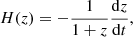
In this context, it is crucial not only to obtain independent measurements of the expansion history of the Universe, but also to find probes that provide such constraints independently of any cosmological assumption. Lately, interest has been growing in the analysis of the oldest astrophysical objects, with the aim of determining their absolute ages, setting a lower limit on the current age of the Universe (Valcin et al. 2021; Cimatti & Moresco 2023), or studying how they age with cosmic time, in an attempt to trace the evolution of the Universe itself (Moresco et al. 2022). This second approach is the so-called cosmic chronometers method (CC; Jimenez & Loeb 2002), which can provide direct estimates of the Hubble parameter from the differential ages of “standard chronometers” with minimal hypotheses. In fact, just assuming the cosmological principle and a Friedmann–Lema tre–Robertson–Walker (FLRW) metric, the Hubble parameter can be expressed as

meaning that it can be directly measured at a given redshift once the local differential of cosmic age (dt) in redshift (dz) is known (an extensive description of the method can be found in Moresco et al. 2022). In order to do this, it is necessary to select a homogeneous and synchronised sample of objects in a certain redshift interval, for which ages or age-related quantities can be measured. In this way, we can obtain an age–redshift that maps the ageing trend of the Universe, and for which Eq. (1) can be applied.
The best astrophysical objects that can be considered cosmic chronometers over a wide redshift range are massive and passively evolving galaxies. A wide range of literature shows that this type of galaxy built up its mass very rapidly (#x0394;t < 0.3 Gyr; Citro et al. 2017; Carnall et al. 2018, 2019; Estrada-Carpenter et al. 2019) and at high redshifts (z > 2 − 3, Thomas et al. 2010; Carnall et al. 2018), so it constitutes a very homogeneous and synchronised population, as with chronometers that started ‘ticking’ coherently. This is of course an assumption whose impact has to be verified directly on the data. Much of the literature undoubtedly points out ongoing star formation in early-type galaxies, mergers, and continuous formation (Moresco et al. 2013; Belli et al. 2017) that, if not properly taken into account, might significantly bias our cosmological analysis.
In light of this, an accurate selection process is required to identify, in a sample of galaxies, a group of chronometers populating the tail of the oldest, most massive objects and not showing any evidence of ongoing star formation. This requires us to analyse different aspects, such as the galaxy’s colour, its spectral features, or the presence of emission lines and their prominence. Many works (Franzetti et al. 2007; Moresco et al. 2018; Schreiber et al. 2018; Borghi et al. 2022a) have proven how these criteria are indeed complementary, and it is necessary to combine them to maximise the purity of the sample.
Other than an accurate selection, the CC method requires robust measurements of differential redshift (dz) and differential ages (dt). While high-precision spectroscopic measurements are today available for the redshift, obtaining accurate age estimates is not as straightforward. Different methods have been explored, some using the whole spectral information – such as full-spectral-fitting (e.g. Carnall et al. 2018) – and others focusing on age-related spectral features (Thomas et al. 2011). In Moresco et al. (2011), another approach was proposed in which, instead of relying on ages, H(z) is determined by tracing the evolution of the break at 4000 Å rest frame (D4000 hereafter), with the advantage of relying on a direct observable. To date, the CC method has been applied up to redshift z ≃ 2, adopting both approaches, and is very promising in view of upcoming large surveys including Euclid (Laureijs et al. 2011), in which the higher statistics will improve the accuracy on H(z) measurements obtained with this technique significantly.
In this work, we took advantage of the deep VIMOS survey of the CANDELS UDS and CDFS survey fields (VANDELS, McLure et al. 2018), which provides optical spectra and photometry of a wide population of galaxies up to z ≃ 6.5. It was designed to provide ultra-deep, medium-resolution spectra, with high enough signal-to-noise ratio (S/N) to perform spectral line studies, both individually on the brighter sources and on stacked spectra for the fainter ones (Garilli et al. 2021). Many works based on VANDELS data have already been published investigating different environments and populations of objects: from the intergalactic medium (IGM; e.g. Thomas et al. 2020, 2021) and active galactic nuclei (AGNs; e.g. Magliocchetti et al. 2020), to Lyα and He II emitters (e.g. Marchi et al. 2019; Hoag et al. 2019; Cullen et al. 2020; Saxena et al. 2020a,b; Guaita et al. 2020) to the physical properties of star-forming (Cullen et al. 2019, 2020; Calabrò et al. 2021, 2022) and quiescent galaxies (Carnall et al. 2019, 2022; Hamadouche et al. 2022). In particular, the last have shown the presence, in VANDELS, of a population of red, massive, and passive galaxies covering the redshift range of 1 ≤ z ≤ 1.5, constituting a potential set of chronometers. Moreover, the richness of spectro-photometric information available in VANDELS allows us to adopt a full-spectral-fitting approach to estimate ages as well as many other physical properties of the sample, such as metallicity and SFH. For this purpose, we took advantage of the public code BAGPIPES (Carnall et al. 2018), which was already tested and validated for VANDELS data, and specifically modified in Jiao et al. (2023) to remove the cosmological prior on ages. All the results obtained in this work are thus independent of any cosmological model.
This paper is divided as follows. In Sect. 2, we present the dataset, the selection process, and the properties of the CCs sample; in Sect. 3 we describe the full-spectral-fitting process and relative results also discussing the impact of different star formation histories assumptions on the results; in Sect. 4 the cosmological analysis is presented, including the H(z) measurement through the CC approach and the assessment of systematic uncertainties; in Sect. 5 we draw our conclusions.
2. Data
In this section, we present an overview of the VANDELS survey, the process adopted to select an optimal sample of cosmic chronometers, their spectral features, and physical properties.
2.1. The VANDELS survey
The VANDELS survey (McLure et al. 2018; Pentericci et al. 2018; Garilli et al. 2021) is a deep VIMOS spectroscopic survey targeting high-redshift galaxies in the CANDELS UDS and CDFS survey fields, with a footprint of ≃0.2 deg2. The observed spectra cover on average the wavelength range 4800 ≤ λ ≤ 9800 Å with a mean spectral resolution R ≃ 650. Both in UDS and CDFS the CANDELS survey (Grogin et al. 2011; Koekemoer et al. 2011) offers deep, optical-near-infrared (nearIR) HST imaging, and in CDFS it also offers deep HST/ACS optical imaging from the GOODS survey (Giavalisco et al. 2004) and ultra-deep X-ray imaging (Luo et al. 2017). However, about 50% of the VANDELS footprint is not covered by HST imaging, which lies only in the central areas, and for those objects in the wider-field region, the optical-nearIR photometric information is provided by different ground-based telescopes. A complete list of the available photometric data, covering the 3700−45 000 Å wavelength range, can be found in Garilli et al. (2021).
In this work, we analysed data from the fourth and final data release of VANDELS (DR4, Garilli et al. 2021), which counts 2087 galaxies pre-selected in photometric redshift to lie in the range 1 ≤ z ≤ 7, comprising 417 star-forming galaxies (SFG, 2.4 ≤ z ≤ 5.5), 1259 Lyman-break galaxies (LBG, 3.0 ≤ z ≤ 7.0), and 278 passive galaxies (PASS, 1.0 ≤ z ≤ 2.5). The remaining 133 objects are AGNs, Herschel-detected galaxies, or secondary objects.
Besides spectra and photometry, DR4 also offers a catalogue including the following: (i) spectroscopic redshift measurements (zspec) and a relative quality flag (zflag); (ii) target classification as one of the types listed above, based on photometric criteria (mainly i, z, H magnitudes and UV and VJ colours) as described in McLure et al. (2018); (iii) spectral-energy-distribution (SED) fitting estimates of object properties, including rest-frame UV and VJ colours, stellar mass, V-band dust attenuation, and star-formation rate (these quantities are derived using the BAGPIPES code Carnall et al. 2018 as described in Garilli et al. 2021; iv) correction factors for the error spectra, introduced to improve the correlation between the variance in the observed spectra and the associated median error, as described in Talia et al. (2023).
The exposure time for each object (up to 80 h) is designed to obtain, especially for passive and star-forming galaxies, a S/N high enough to perform detailed spectroscopic studies. This consists of a S/N higher than ten for star-forming and passive galaxies, and higher than five for the other targets (Garilli et al. 2021).
2.2. Selecting a reliable sample of cosmic chronometers
A proper application of the cosmic chronometers method requires the selection of the purest sample of massive and passively evolving galaxies, avoiding contamination by younger star-forming objects that could bias the subsequent cosmological analysis (see Moresco et al. 2022 for more details). Many different criteria have been developed for this purpose, based on rest-frame colours (e.g. UVJ, Williams et al. 2009; NUVrJ, Ilbert et al. 2013), SED (e.g. Ilbert et al. 2010), star-formation rate (SFR; e.g. Pozzetti et al. 2010), or emission lines (e.g. Mignoli et al. 2009). In this context, several works have also shown that adopting a simple criterion is not enough to identify all the possible star-forming outliers, with possible residual contamination of up to 50% depending on the criterion (Franzetti et al. 2007; Moresco et al. 2013).
For this reason, aiming to maximise the purity of our sample, in this work we combine different and complementary cuts, based on both photometric and spectroscopic information, following this outline:
(1) Parent sample. as a starting point, we define a parent sample made of galaxies selected as follows. As a first step, we select galaxies classified as passive targets in VANDELS (278 objects). Among the passive targets, we consider galaxies in the redshift range of 1.0 ≤ z ≤ 1.5 (241 objects), with the lower and upper boundaries of the redshift interval excluding, respectively, four and 33 objects. The lower limit is applied because the distribution of the passive sample becomes statistically significant at z ≥ 1. The upper limit, given the spectra wavelength coverage, is needed to ensure that all spectra include some major spectral features, such as the D4000 break, that are crucial in the following analysis.
Lastly, we require zflag = 3, 4. In VANDELS, this flag identifies objects with the most reliable redshift measurements; these are estimated to have a > 99% probability of being correct (Garilli et al. 2021). This requirement, met by 265 passive targets, is particularly relevant for the cosmological analysis. Combining the aforementioned criteria, the parent sample counts 234 galaxies.
(2) UVJ cut. since the DR4 catalogue provides rest-frame U − V and V − J colours, we apply the photometric criterion based on the colour–colour UVJ diagram (Williams et al. 2009) in order to select photometric passive galaxies, adopting the cut in McLure et al. (2018):
As mentioned before, this criterion was already used for the target classification, but the U − V and V − J colours, in that case, were slightly different from those available in the DR4 catalogue. In both cases, they are derived via SED-fitting, but in DR4 this is performed with the additional information of spectroscopic redshifts, an improved photometry, and the BAGPIPES code, optimised for this survey. By applying the UVJ cut on the parent sample, 25 additional objects are discarded. Most of them were identified as post-starburst galaxies in Carnall et al. (2019). After the UVJ selection, our sample is reduced to 219 galaxies.
(3) [OII] cut. we further clean the sample by analysing the [OII]λ3727 emission line, an indicator of ongoing star formation since it is a tracer of photo-ionised gas (Magris et al. 2003). A cut on the equivalent width (EW) of the [OII] is often adopted, as in Mignoli et al. (2009), where star-forming objects are identified by EW([OII]) > 5 Å. In this work, a more conservative choice was preferred, and only galaxies with a significantly detected [OII] line are discarded, namely objects with EW([OII]) > 5 Å and S/N([OII]) > 3. This means that spectra with EW([OII]) > 5 Å but low S/N are not excluded from the sample, with the aim being to keep objects in which the [OII] line could simply be due to noise fluctuation.
The [OII] cut turns out to be the most restrictive selection step, reducing the sample to 96 galaxies (41% of the parent sample), but is fundamental to minimise the contamination by ongoing star formation or younger components, as discussed in Moresco et al. (2022).
(4) H/K cut. Another stellar population diagnostic is the ratio of two absorption lines, CaII H at 3969 Å and CaII K at 3934 Å, first defined by Rose (1984). In passive galaxies, the CaII K line is generally deeper than the CaII H, but since the CaII H line overlaps with the Hϵ line of the Balmer series at 3970 Å, deeper in the presence of young and hot A and B-type stars, CaII H results more prominent than CaII K if a young component is present in the population. Recent works (Moresco et al. 2018; Borghi et al. 2022a) have proven the effectiveness of this indicator by showing that a 5% contamination by young populations in the flux budget triggers the inversion.
To quantify this behaviour, we evaluate the ratio H/K ≡ (CaII H + Hϵ)/CaII K by measuring the corresponding pseudo-Lick indices with the code PyLick (Borghi et al. 2022a). When using integrated quantities, a common requirement to identify non-contaminated objects is H/K < 1.2−1.5 (Borghi et al. 2022a). In this work, we selected galaxies with H/K < 1.3 in order to increase the purity of the sample preserving the statistics, as can be seen in Fig. 1f. The H/K cut reduces the sample to 78 galaxies.
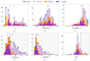 |
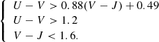
Fig. 1. Histograms for the physical and spectral properties of the samples in each selection step, as shown in the legend and described in Sect. 2.2. Vertical arrows represent the corresponding median values, and, when present, the dashed vertical line indicates the threshold value adopted to select cosmic chronometers according to that quantity (the shaded area showing the discarded range). We note that for the [OII] we adopted a conservative cut, discarding only the objects that showed both EW([OII]) > 5 Å and S/N([OII]) > 3, aiming to keep objects in which the [OII] line could be due to noise fluctuation. |
(5) Visual inspection. The remaining spectra are visually checked to search for anomalies such as residual emission lines or calibration issues. We identify four objects showing this kind of issue: CDFS128563, UDS000769, UDS021218, and UDS137225. After this step, the sample counts 74 galaxies.
(6) Redshift cut. On the selected sample, we first perform a study of the spectral features, to which we dedicate the next section. This analysis highlights an anomalous behaviour with redshift of some spectral features, making it necessary to add a further selection step. In particular, we find that all objects below redshift z < 1.07 present a 4000 Å break (D4000) weaker than its expected value at those redshifts, with an inconsistent evolutionary trend, which appears to be caused by some systematic effect. Several possible causes for this effect have been explored and are extensively discussed in Appendix A; however, up to now no clear evidence has been found to account for this anomaly. For this reason, to avoid introducing a potential bias in the subsequent cosmological analysis, we prefer to discard the 23 galaxies below this redshift threshold. We highlight that this does not affect the robustness of the following results since it only reduces the redshift coverage.
Finally, we cross-checked our galaxies with the VANDELS AGN sample (Bongiorno et al., in prep.), removing two objects which are identified as AGNs. We thus obtain a final sample of 49 cosmic chronometers.
In Table 1, median values for different physical and spectral properties are listed for each step of the selection process. Unless otherwise specified, errors on median values are computed as median absolute deviations (MAD) divided by the square root of the number of objects. The S/N for each spectrum is estimated as the median of the S/N computed in each pixel in the range 3100 < λ < 3500 Å. In Fig. 1, the distribution of some of these properties for each passage is shown. Using the same colour-code, in the top panel of Fig. 2 we show the UVJ diagram, and in Fig. 3 we show the median stacked spectra for each selection step (normalised in the wavelength range of 3320−3850 Å). In the bottom panel of Fig. 2, we show the EW[OII] against the H/K ratio for the sample obtained after the UVJ cut. This highlights how the two selection steps act in clearing the sample. In particular, we can observe that the threshold we adopted in EW[OII] and the one in S/N[OII] match very well, meaning that we are discarding galaxies where this emission line is really present and evident.
 |
Fig. 2. Photometric and spectroscopic selection criteria. Top: UVJ diagram for the main selection steps. Galaxies above the dashed line are qualified as passive following the criterion in McLure et al. (2018). Bottom: EW[OII] versus H/K ratio, colour-coded by S/N[OII], for the sample after the UVJ cut. The shaded areas show the discarded ranges for both quantities. |
 |
Fig. 3. Median stacked spectra estimated for the different incremental selected samples of our analysis, as described in Sect. 2.2. We underline that the final sample considered is the purple one, on which we also highlight the most characteristic absorption features (grey shaded area) and spectral breaks (dashed area), as well as the position of potential emission lines (red shaded area), showing the absence of emission lines in our final sample. |
The selected sample of cosmic chronometers, with a median redshift of ⟨z⟩ = 1.21 ± 0.02, populates the tail of the reddest galaxies in the UVJ diagram and shows the required properties. In particular, it has a median stellar mass equal to ⟨log(M⋆/M⊙)⟩ = 10.88 ± 0.05, and about 75% of the sample has log(M⋆/M⊙) > 10.6, a value often used as a threshold to select CCs (Moresco et al. 2022). The median specific star formation rate (sSFR) is ⟨log(sSFR/yr−1)⟩ = −12.2 ± 0.2, and more than 90% of the sample has log(sSFR/yr−1) < − 11, a common limit to characterise passive galaxies (Pozzetti et al. 2010). The histograms in Fig. 1 also show how the selection based on spectral features has been effective in minimising the contamination by young stellar activity, decreasing the sSFR obtained after only the UVJ cut by 90%. The distributions in [OII] and H/K are typical of passive populations too, with a typical S/N([OII]) < 3 and a median ⟨H/K⟩ = 0.92 ± 0.02 well below the adopted threshold. In Fig. 1d, one can also see the presence of a few objects that, despite having EW[OII] > 5 Å, are kept in the CCs sample because of the low S/N[OII].
In Fig. 3, the effect of the selection process is shown on median composite spectra. Top-down, the blue stacked spectrum, relative to the parent sample, has the most prominent [OII] emission and very similar CaII H and CaII K. The lilac one, realised after the UVJ cut, is not much different because the sample differs only by 25 objects, mostly post-starburst galaxies (Carnall et al. 2019), but shows a slightly weaker [OII]. Anyway, this confirms again how just adopting a photometric criterion is not enough to remove the contamination by young components, because the [OII] emission line, even if weak, is still present. Only the cut on its EW, which leads to the orange spectrum, is able to clean out this feature. It has a sharp impact on the statistics but is necessary to maximise the purity of the sample. Finally, the purple spectrum is built with the 49 CCs and, besides showing no [OII] emission, has the minimum H/K ratio.
2.3. Spectral properties of the CCs sample
Since the CCs sample falls in the redshift range of 1 < z < 1.5, the spectral coverage is able to include some interesting spectral features. One of the most relevant is the D4000, a spectral discontinuity at 4000 Å, which is particularly strong in the context of passive galaxies. It is caused by a sudden onset of absorption lines at wavelengths bluer than 4000 Å and is stronger in evolved stellar populations. For this reason, at fixed metallicity, it has a tight correlation with the galaxy age -with older galaxies having a stronger D4000 – and a very low dependence on the presence of α-elements (Moresco et al. 2012). The classical definition of the D4000 is given in Bruzual (1983), while more recent is the narrow definition (Dn4000) given in Balogh et al. (1999), which is less affected by dust absorption. This last one is shown in the purple spectrum in Fig. 3.
As with the CaII H and K, we use PyLick to measure the Dn4000 for the whole sample of CCs. In order to study its trend with redshift and mass, we separate high-mass (HM) and low-mass (LM) galaxies by the median stellar mass of the sample, 1010.88 M⊙. We then divide each sub-sample into three redshift bins, such that there is the same number of objects in each bin, obtaining a total of six sub-samples. In each of them, we measure the median Dn4000 value. In Fig. 4, we show Dn4000 measurements obtained for single galaxies (grey) and median values in each sub-sample: in blue for the LM sample, in red for the HM sample. The Dn4000 shows a clear decreasing trend, both for the HM and the LM samples, providing initial observational evidence that the selected CCs sample ages with cosmic time. We also observe a mass-downsizing trend (Thomas et al. 2010), given that HM galaxies have a stronger median Dn4000 than LM objects at fixed redshift. These results constitute a first observational validation of the core hypotheses of the CC method.
 |
Fig. 4. Dn4000 trend with redshift. The measurements for the single objects of the CCs sample are shown in grey; blue and red dots are median values averaged in two mass bins, log(M⋆/M⊙)≤10.88 (high-mass) and log(M⋆/M⊙) > 10.88 (low-mass), respectively. The different lines show the Dn4000–z relation obtained from the 2016 version of the Bruzual & Charlot (2003) models at different formation redshifts and assuming a reference flat ΛCDM cosmology (ΩM = 0.3, ΩΛ = 0.7 and H0 = 70 km s−1 Mpc−1), purely for illustrative purposes. We note that, qualitatively, the observed trends follow the cosmological models quite well, but we defer to Sect. 4 the full cosmological analysis. |
3. Method and analysis
In this section, we present the method adopted to estimate ages and physical properties of the CCs sample, the code used, its settings, and the results obtained.
3.1. Full spectral fitting with BAGPIPES
Today there are two main ways of estimating ages from galaxy spectra: by fitting observed spectra with synthetic ones, and so using the whole spectral information, or by focusing on particular age-dependent indices. In this work, to benefit from the richness of the spectral and photometric information available in VANDELS, we followed the first path. In particular, we exploited a full-spectral-fitting technique using the public code BAGPIPES (Carnall et al. 2018) – already employed and optimised on VANDELS data- which allowed us to fit jointly spectra and photometry with a Bayesian approach. This means that once we have chosen a model ℳ depending on a set of parameters θ, the observed spectrum fλ is modelled to maximise the posterior probability on θ, 𝒫(θ|fλ, ℳ), as defined by the Bayes theorem,
and sampled through the nested sampling algorithm MultiNest (Buchner 2016). In particular, as extensively described in Carnall et al. (2019), the model is built with four main components.
The first is SSP(λ, age, Z), a simple stellar population model depending on the wavelength λ, on the age of the stellar population, on its metallicity Z, and on the initial mass function (IMF). The stellar population synthesis (SPS) models, implemented in the form of grids of SSPs, are the 2016 version of Bruzual & Charlot (2003, BC16; see Chevallard & Charlot 2016). They are constructed using a Kroupa (2001) IMF.
The second is SFR(t), which is the galaxy star formation history (SFH). The code allows us to combine different SFHs, one for each SSP, with various functional forms (e.g. delta function, constant, exponentially declining, double power law).
The third is T+(age, λ), which is the transmission curve of the ionised interstellar medium (ISM) as described in Charlot & Longhetti (2001). This component is referred to as nebular and, unlike the ones above, is optional.
The fourth is the T0(age, λ) transmission curve of the neutral ISM, which is mainly due to dust absorption and emission. Different models are implemented in the code, including those of Calzetti et al. (2000), Cardelli et al. (1989), or Charlot & Fall (2000). This is also an optional component and is referred to as dust. In addition to these, there are two more optional but non-physical components: noise, which is an additive term acting on the error spectrum to correct a possible underestimation; and calibration, which perturbs the spectrum with a second-order Chebyshev polynomial to fix possible calibration issues.
The code provides, for each galaxy, a best-fit spectrum and an estimate to the 16th, 50th, and 84th percentiles of all the parameters involved in the fit (e.g. age, metallicity, and stellar mass formed). The Mformed parameter is defined as the whole stellar mass formed from t = 0 to the time t at which it is observed:
In the following, we refer to this parameter when discussing the mass of the galaxies. This parameter is slightly different from the standard stellar mass, which does not include stellar remnants, but the two are tightly correlated. In general, we find an offset of ∼0.2 dex between the two, which we need to take into account when comparing our resulting masses with literature values.
In this context, it is important to underline that the version of BAGPIPES we are using differs from the original for the treatment of the prior on galaxies’ ages. This modification is described in detail in Jiao et al. (2023). Originally, the code assumed a cosmological prior on ages, for which the maximum age of the fit should be smaller than the age of the Universe at the corresponding redshift, given a flat ΛCDM model with the parameters ΩM = 0.3, ΩΛ = 0.7 and H0 = 70 km s−1 Mpc−1. Although its impact is of relative interest in galaxy evolution studies and is generally neglected, it cannot be ignored in cosmological analyses because the derived ages would be constrained by the cosmological model assumed; hence, when fitting those, one would just retrieve the assumed prior. To avoid this, we consider instead a uniform prior on galaxy ages, so that they can span between 0 and 20 Gyr independently of redshift. This implies that, in theory, the estimated ages could result more advanced than the age of the Universe expected in a standard cosmological model at a given redshift, so a first test will be to verify their compatibility.
BAGPIPES is able to combine multiple SFHs, one for each stellar population, with different functional forms. Here, we present two of the most extensively used, on which we focus our analysis.
The delayed exponentially declining (DED) SFH, is given by the equation
where τ sets the width of the SFH while T0 is the age of the Universe when the star formation begins. This means that it is directly linked to the age of the galaxy, which can be obtained by

where ageU(zobs) is the age of the Universe at the redshift of observation. Besides this, BAGPIPES provides another age definition called mass-weighted age:
This is similar to Eq. (6), but T0 is replaced with an estimate of the age-weighted on the galaxy SFR. In the case of a DED SFH, the results obtained with these two definitions differ by an offset (∼0.6 Gyr), typically constant in redshift and age.
This SFH is frequently used (Citro et al. 2017; Carnall et al. 2018) for passively evolving galaxies, characterised by a single and strong episode of star formation followed by passive evolution, because it is able to reproduce a realistic star formation process using only two parameters.
The double-power-law (DPL) SFH, given by
![$$ \begin{aligned} {\mathrm{SFR}(t)} \propto {\left[\left(\frac{t}{\tau }\right)^\alpha + \left(\frac{t}{\tau }\right)^{-\beta }\right]}^{-1}, \end{aligned} $$](/articles/aa/full_html/2023/11/aa46992-23/aa46992-23-eq10.gif)
where α and β describe, respectively, the falling and rising slope of the curve while the τ parameter is related to the SFH peak. In this case, differently from a DED SFH, due to the shape of the SFH, the only age definition provided is the mass-weighted one. This type of functional form allows the SFH more freedom in shape by decoupling the rising and falling phase of the star formation, but the increased number of free parameters should be carefully studied since it might induce a non-physical correlation between the two (see Appendix B).
3.2. Full spectral fitting in VANDELS
Before performing the fit on VANDELS data, we checked spectra and photometry to fix possible anomalies. On the one hand, we define a spectroscopic S/N by dividing, at each wavelength, the flux for its associated noise, which allowed us to determine the average S/N of the spectrum. On the other hand, analysing the photometric S/N distribution, we observe that it is up to three orders of magnitude higher (max(S/Nphot)∼103) than the spectroscopic one (⟨S/Nspec⟩ = 5.74 ± 0.17) for the same object, especially at the reddest wavelengths. If unaccounted for, this difference can have a significant impact on the fit, forcing it to reproduce the photometry irrespectively of the spectroscopic data. We also observe that the redder photometric points are also the ones with smaller errors, and this could introduce an additional bias in the analysis since the bluer photometric data points have also been proven to be fundamental in reconstructing the physical properties linked to the star-formation activity. To correct for this issue, we assumed a maximum S/N for the photometric data points to S/N = 10, correcting the errors in case it was larger and in this way better weighting all the parts of spectrum and photometry.
Once we had performed these corrections, we tested different configurations of parameters and priors, with a particular focus on the impact of the chosen SFH. This is important not only to accurately reproduce the observed data, but also to evaluate how robust the results are when changing the fitting model, which is fundamental to estimate potential biases and systematic effects when performing cosmological analyses. Here, we report parameters and priors of three fit settings: baseline, configuration 1, and configuration 2, as reported in Table 2. They mainly differ in two characteristics: the SFH functional form and the data used in the fitting process. The baseline and configuration 1 models both fit spectra and photometry, but with a different SFH: respectively a DED and a DPL; the baseline and configuration 2 models both use a DED SFH, but the second one does not include photometry in the fit. Apart from these differences, all these three models are built on a common set of components, namely: (i) a SFH modelled either with a DED or a DPL functional form; (ii) a dust attenuation component described in Salim et al. (2018), which consists of a power law as in Calzetti et al. (2000), but with a deviation from the slope parameterised by δ; (iii) a nebular component implemented in BAGPIPES using the code Cloudy (Ferland et al. 2017) and described in more detail in Carnall et al. (2018; the process of selection should have already excluded objects having this type of emission, but we conservatively decided to include it in the model to verify its absence); (iv) redshift fixed, for each galaxy, to the value of the spectroscopic redshift obtained in VANDELS; (v) a calibration component, implemented as a second-order Chebyshev polynomial; (vi) a noise correction, introduced as white noise. The main parameters and relative priors are listed in Table 2.
Parameters and priors adopted for each configuration used in the full spectrum fitting.
For each configuration, we verified the convergence of the results and that the best-fit model is correctly reproducing the observed spectra and photometry. If these requirements are not met, the results cannot be considered valid, and they are therefore flagged as a bad fit. To perform this operation, we visually examined the best-fit spectra and photometry and the distribution of the posterior probability on the parameters for each galaxy. For the baseline configuration, only 5/49 galaxies are flagged as bad fits. In Fig. 5, the typical best-fit spectrum and photometry are shown in the case of a good fit for the baseline configuration.
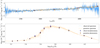 |
Fig. 5. Example of best-fit spectrum and photometry (in orange) obtained by fitting the observed ones (in blue) with the baseline configuration, as described in Sect. 3.2. |
As the name implies, the baseline configuration will be used as a benchmark to perform both the analysis of the physical properties of the population and the cosmological study, which is presented in the next sections. Among the three configurations presented here, it presents the smaller number of bad fits and the best agreement between observed spectrophotometry and the posterior one. In Appendix B, we instead discuss the comparison between baseline and configuration 1 results, aiming to evaluate how the choice of a more complex SFH impacts the results. This also allows us to account for its systematic effect in the cosmological analysis.
3.3. Physical properties of the CCs sample
The fitting process with the baseline configuration is successful for 44 CCs (90% of CCs sample), with a median reduced chi-square of  = 1.46, considering both spectra and photometry. In order to estimate their physical properties, we computed, for each parameter, the median and 16th–84th percentile ranges of the posterior distribution. The analysis of these quantities shows that our CCs sample, in agreement with our selection process, consists of galaxies with high stellar masses, as commonly occurs in a population of passive galaxies, with a median stellar mass ⟨log(Mformed/M⊙)⟩ = 11.21 ± 0.05; a median metallicity value of ⟨Z/Z⊙⟩ = 0.44 ± 0.01; short SFHs, with a typical timescale for the star formation ⟨τ⟩ = 0.28 ± 0.02 Gyr, which also agrees with a mass-downsizing scenario where more massive galaxies are the first to assemble in very short bursts of formation (Thomas et al. 2010; Citro et al. 2017); and low dust reddening, with a median V-band dust extinction of ⟨AV, dust⟩ = 0.43 ± 0.02 mag.
We notice here that in the literature there is quite a large spread in the derived metallicity for passive and massive galaxies at these redshifts, with estimates going from sub-solar values of 0.4−0.7 Z⊙ (e.g. Kriek et al. 2019; Lonoce et al. 2020; Carnall et al. 2022) up to 1.3−1.6 Z⊙ (e.g. Conroy et al. 2014; Onodera et al. 2015). Our results, in particular, are compatible with the ones found in Kriek et al. (2019) and Lonoce et al. (2020), and slightly lower with respect to the metallicities obtained by Carnall et al. (2022), who analysed the stacked spectra from a sample of VANDELS passive galaxies in the range 1 ≤ z ≤ 1.3, finding 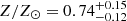 with BAGPIPES.
We also compare our results with the independent analysis of Saracco et al. (2023), who studied a sample of 64 passive galaxies in VANDELS performing non-parametric full-spectral-fitting on stacked spectra in six mass ranges, using different combinations of models and fitting codes. The sample was selected following the same requirements adopted in this work to identify the parent sample but with a tighter redshift range (1 ≤ z ≤ 1.4) and adding a lower limit to the S/N (S/N > 6 per Å in the range [3400−3600] Å). They find typically over-solar metallicities, different from both the ones in this work and in Carnall et al. (2022). The spread in these results could be due to the models adopted or to the full-spectrum-fitting code used, as also shown in Saracco et al. (2023), where the variation of one or both of them produces a scatter in the metallicity estimation of up to 0.4 dex.
It is important to underline that, for the cosmological purpose of this work, we expect the impact of this effect to be negligible, given that the CC method relies on the estimation of differential quantities. In particular, given an optimally selected sample of massive and passive galaxies, what is fundamental is ensuring its homogeneity. This condition is met in our sample, which shows homogeneous metallicities in the considered redshift range. Moreover, comparing our age estimates with the ones in Saracco et al. (2023), we find a good agreement with their mass-weighted ages, using both the STARLIGHT (Cid Fernandes et al. 2005) and pPXF (Cappellari 2017) codes.
By adopting an archaeological look-back approach, we can study how our measured quantities vary as a function of redshift. In particular, given the cosmological purpose of this work, we are interested in the age–redshift relation, which is discussed in detail in Sect. 3.4. In Fig. 6a, we show the age–redshift for our 44 CCs coloured by stellar mass. From this trend, we can draw three main conclusions. First, for most of the galaxies (95% of CCs), ages are below that of the Universe, as expected in a standard cosmology (flat ΛCDM with ΩM, 0 = 0.3, ΩΛ, 0 = 0.7, H0 = 70 km s−1 Mpc−1), even without having imposed a cosmological prior, since they could formally vary between 0 and 20 Gyr across the entire redshift range. This is, perse, a significant result since it demonstrates that with enough spectral coverage, a sufficient S/N, and adequate photometric data, we can constrain this parameter reliably without any additional cosmological assumption. Second, the ages show a decreasing trend with redshift in agreement with the cosmological expectation, in line with what was already observed for the Dn4000. The third important observation is the existence of a mass-downsizing trend, with more massive galaxies being older than the less massive ones at fixed redshift. In particular, objects with log(Mformed/M⊙) ≤ 11.1 show formation redshifts in the 1.5 ≲ zform ≲ 4 range, while for galaxies with log(Mformed/M⊙) > 11.1 it spans the 2 ≲ zform ≲ 7 range.
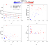 |
Fig. 6. Trends with redshift of age (a), stellar mass (b), tau parameter (c), and metallicity (d), colour-coded by stellar mass. In the age–redshift the lines in the background represent the theoretical trends in a flat ΛCDM cosmology with ΩM, 0 = 0.3, ΩΛ, 0 = 0.7, H0 = 70 km s−1 Mpc−1, and different formation redshifts. |
In Fig. 6, we show the trends with redshift for other relevant physical parameters estimated in the fit (stellar mass, metallicity, and τ parameter), coloured accordingly to the stellar mass. We can notice that for the more massive sample (in red) there are no strong trends with redshift for any of the considered quantities, except the ages, while the lower mass sample (in blue) shows a mild increasing trend with redshift for the stellar mass. This is a well-known effect due to the observational luminosity threshold, which allows us to see only the intrinsically brightest objects when we observe the distant Universe. This effect can be noted in particular for the stellar mass since it correlates with the galaxy luminosity. Given this, it is clear that to obtain a homogeneous sample as a function of redshift for the cosmological analyses, it will be necessary to perform a cut in stellar mass, as we discuss in Sect. 3.4.
Another important observation in this context can be derived for the τ parameter, which is related to the SFH length, and its trend with redshift in Fig. 6c. Both for the higher and the lower mass galaxies it is stable around 0.3 Gyr, but the high-mass sample seems to have a longer period of star formation, in contrast with what is expected in a mass-downsizing paradigm, in which the more massive a galaxy is, the older it is expected to be, and the shorter its SFH. We trace the origin for this inversion to be the existent degeneracy between τ and age, occurring as a direct correlation between these two parameters. This effect is well known in literature (Gavazzi et al. 2002) when adopting a DED SFH, since age and τ have very similar effects on the spectral shape, and it is difficult to disentangle their contribution. The impact of this effect, however, is negligible on our results since the range of retrieved τ is extremely small and compatible with a very short SFH, and, most importantly, because our cosmological analysis is made on sub-samples with constant mass and where the τ appears very stable as a function of redshift. In this context, it is even more interesting to analyse the impact on the results of adopting a DPL SFH, in which the decoupling of the rising and falling slope allows more freedom for the SFH shape.
The assumed SFH has been identified in recent literature as a potentially significant source of systematic effects in the estimate of galaxies’ physical parameters. For this reason, we extensively tested the dependence of our measurements on the assumed SFH functional form. In particular, we repeated our analysis considering the DPL SFH (configuration 1) and assessed the robustness of our results. In Appendix B, we provide a detailed discussion of our findings. In summary, we obtain that the age estimates are very robust, with minimal variations occurring when changing the SFH. In particular, setting a lower limit to the rising slope of the DPL SFH (β > 10) to exclude non-physical solutions, we find a median percent difference in age estimates below 2%. In terms of velocity dispersion and dust reddening, the discrepancy is even smaller, reaching a median percent difference lower than 1%, while the gap in stellar mass is of 0.001 dex. Moreover, the resulting SFH shapes are almost identical when adopting a DED or a DPL, despite the different functional forms. In the following sections, we use the results of configuration 1 to assess the systematic effect introduced by assuming a different SFH in estimating the cosmological parameters.
3.4. Optimising the selection of cosmic chronometers
In Sect. 3.3, the discussion of the physical properties of the 44 selected galaxies has provided additional support to the fact that these objects meet the conditions for being CCs, given their high masses (⟨log(Mformed/M⊙)⟩ = 11.21 ± 0.05) and their very short periods of star formation ⟨τ⟩ = 0.28 ± 0.02 Gyr. At this point, an important aspect to be considered in applying the method is the maximisation of the synchronicity of the sample formation time. In a mass-downsizing scenario, high-mass galaxies (the cut log(M⋆/M⊙) > 10.6 is often applied; Moresco et al. 2022) are the first to form (z > 2 − 3, Citro et al. 2017; Carnall et al. 2018, 2019) in a short burst of star formation (t < 0.3 Gyr, Thomas et al. 2010; Carnall et al. 2018), so they are the best able to provide a sample of synchronised chronometers. Anyway, it is important not only to select massive galaxies, but also that their properties be consistent in redshift in order to maximise the homogeneity of the sample at different cosmic times and to avoid biases in the cosmological analysis. In the previous section, commenting on Fig. 6, we note that the sample shows homogeneous metallicity and τ throughout redshift, while the stellar mass for the low-mass sample – in blue in Fig. 6b – shows an increasing trend with redshift. Then, with the aim of homogenising the sample mass, we apply a further cut log(Mformed/M⊙) < 10.8 (discarding 5 galaxies), a threshold that not only makes our CCs homogeneous in mass, but also in redshift of formation, removing all the galaxies with zform < 2 in Fig. 6a. The sample of CCs that we adopted for the cosmological analysis thus features 39 galaxies.
With this accurately selected sample, we were then able to build the median age–redshift relation, which is more robust in tracing the ageing trend since it allows us to increase the S/N of our measurements. This consists of dividing the sample into redshift bins and eventually into mass bins, and then averaging ages and redshifts in each sub-group. To each median age, we assigned an error computed as MAD/ . We tested different types of binning: (i) equally spaced or equally populated in redshift; (ii) two or four redshift bins; (iii) sub-dividing (or not) the sample into mass bins according to the median value of the log(Mformed/M⊙) distribution (⟨log(Mformed/M⊙)⟩ = 11.26). When dividing the sample into mass sub-samples, we decided to split them in redshift bins after the mass separation to obtain more homogeneous sub-samples in mass, and, hence, time of formation.
By combining these three options, eight different binning types can be obtained, but not all of them are effective in tracing the age–redshift trend. For example, using the separation in mass and four redshift intervals at the same time produces a total of eight sub-samples with ≤5 galaxies each, ending with median values that are very sensitive to fluctuations in each bin. On the contrary, adopting two redshift bins and no mass separation would lead to more stable median values, but having just a pair of points is not effective in constraining the age–redshift trend. Additionally, aiming for the maximum synchronicity of the population that we average on, we find it better to always adopt the mass separation, which guarantees a better homogeneity of the sample in each bin.
After these considerations, we can conclude that the best binning types for our sample are two, given by two equally spaced or equally populated redshift bins, divided in mass. We refer to the equally spaced one as binning A, which we use as a benchmark, while the equally populated one is referred to as binning B and is used as a comparison. This choice was made because the first one guarantees a more homogeneous sampling of the ageing trend also in terms of redshift. The median age–redshift trend for binning A is shown in Fig. 7 and the relative median values and errors are reported in Table 3.
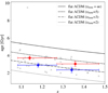 |
Fig. 7. Median age–redshift trend for the 39 CCs sample, obtained with binning A. Red and blue dots represent median values, respectively, for the high-mass (log(Mformed/M⊙) > 11.26) and the low-mass (log(Mformed/M⊙)≤11.26) sample. In the background, grey dots are the 39 single measurements, while lines show, for illustrative purposes only, the theoretical trends with different redshifts of formation, as given by a flat ΛCDM model with ΩM = 0.3, ΩΛ = 0.7 and H0 = 70 km s−1 Mpc−1. |
Median ages and properties of the selected CC sample considering the binning A as described in the text.
4. Cosmological analysis
In this section, we describe the use of the median age–redshift relation built in Sect. 3.4 to perform the cosmological analysis. In particular, we applied the cosmic chronometers method, directly measuring the Hubble parameter using Eq. (1) that does not rely on any cosmological model. In this way, we obtain a new estimate for H(z) at redshift z > 1 that is completely cosmology-independent. As an additional test, we also considered fitting the age–redshift relation directly, assuming instead a cosmological model. This allowed us to derive an estimate of the Hubble constant H0, which is not, however, cosmology-independent. We note here that it could be also possible to derive a cosmology-independent estimate of H0 by extrapolating the H(z) relation down to z = 0 (Moresco et al. 2022; Moresco 2023).
4.1. Cosmological constraints with the cosmic chronometers approach
Starting from the median age–redshift relation obtained in Sect. 3.4, we were then able to apply the cosmic chronometers method. As already discussed in Sect. 1, the Hubble parameter H(z) can be estimated by evaluating the differential age evolution over a small redshift bin dz of a sample of cosmic chronometers through the equation
which means that we can estimate the Hubble parameter at the redshift of the CCs sample by measuring the first derivative of the age–redshift relation. This requires an accurately synchronised sample of CCs; a suitably large redshift interval, such that the differential in age (dt) is larger than its uncertainty; and small age errors, to maximise the accuracy on the measurement of dz/dt. The selection process presented in Sect. 2.2 and the optimisation of the CCs sample in Sect. 3.4 showed that the 39 selected CCs have the characteristics to satisfy the first requirement. Moreover, the chosen binning type (binning A, described in Sect. 3.4) is optimal for meeting these requisites, representing a good balance between the need for sampling in redshift and the need for statistics in each bin. At the same time, adopting the mass separation allowed us to maximise the synchronicity of each sub-sample given the strong correlation among stellar mass, age, and redshift of formation expected in a mass-downsizing scenario (Thomas et al. 2010).
4.1.1. Computing H(z) with the cosmic chronometers method
Starting from the median age–redshift relation obtained with binning A, shown in Fig. 7 and reported in Table 3, the Hubble parameter H(z) is computed in two steps: first, Eq. (9) is applied separately on the two high- and low-mass data points, where z is computed as the mean redshift of the two points, obtaining two H(z) measurements and relative errors; then we compute the average of these two values, weighted on the associated error. We can obtain this average because, while the median age in the two mass sub-samples is clearly offset due to a different time of formation, and hence needs to be analysed separately, the underlying cosmology has to be the same, and therefore the Hubble parameter estimates can be averaged to increase the accuracy of the measurement. In this way, we obtain an estimate for the Hubble parameter at z ≃ 1.26:
![$$ \begin{aligned} H(z \simeq 1.26) = 135 \pm 60\,(\mathrm{stat}) \quad [\mathrm{km\,s^{-1}\,Mpc^{-1}}], \end{aligned} $$](/articles/aa/full_html/2023/11/aa46992-23/aa46992-23-eq15.gif)
where the associated error is given here by the only contribution of the statistical uncertainty, resulting from the propagation of the error on median ages, which scales with  , the number of elements in each bin. In the next section, we analyse the impact on the result of two effects, the binning choice, and the SFH choice, aiming to include a systematic component in the uncertainty.
4.1.2. Study of the systematic effects on H(z)
In Sect. 3.1 we discuss the different types of fit configurations that have been tested on our CCs sample. We pay particular attention to configuration 1, which differs from the baseline in having a DPL SFH instead of a DED SFH, to which Appendix B is dedicated. There, we find a strong agreement between baseline and configuration 1 results with a mean percentage difference in ages smaller than 2%. Here, we want to understand how this slight discrepancy in age propagates to the estimation of the Hubble parameter. We should recall that when using a DPL SFH, BAGPIPES only provides mass-weighted ages, as defined in Eq. (7), while baseline results are built with standard ages, from the definition in Eq. (6). As already discussed, this difference does not introduce a change in the slope of the ageing trend, because we verify that the offset between the two definitions is constant in redshift.
After performing the fit with configuration 1, we discarded the five objects identified in Sect. 3.4 to have log(Mformed/M⊙) < 10.8, and then we cleared bad fits from the sample, ending up with a sample of 36 CCs. With these, we obtain a new median age–redshift by applying binning A, and then we implemented the CC method by repeating the process explained in Sect. 4.1. The Hubble parameter measurement in this case is H(z ≃ 1.25) = 156 ± 51 km s−1 Mpc−1.
To include the effect of the assumed binning in the total error budget, we repeated this process for binning B, both with baseline and configuration 1 results. The four measurements obtained are reported in Table 4. To estimate the impact of choosing a different SFH, we computed the average difference between baseline and configuration 1 measurement of H(z) for equivalent binnings, which results in a contribution to the error budget of #x0394;HSFH = 27 km s−1 Mpc−1. We note that this large uncertainty is dominated by the H(z) value obtained with configuration 1 and binning B, the less accurate of the four estimates that we derive, as shown in Table 4. This effect is due to the fact that in this configuration the number of correctly estimated ages is smaller than in the baseline configuration, and therefore, with the statistics being lower, it is subject to slightly larger fluctuations when varying the binning. In particular, we notice that by choosing the equally populated binning we end up with an uneven redshift sampling that increases the fluctuation in the average ages, resulting in a significantly larger uncertainty on H(z). If we exclude this result, #x0394;HSFH would be cut down to 15 km s−1 Mpc−1. Lastly, we also included the discrepancy in H(z) between baseline binning A and binning B, #x0394;Hbin = 2.4 km s−1 Mpc−1, in the error. Adding these two contributions, we obtain the following:
![$$ \begin{aligned} H(z \simeq 1.26) =&135 \pm 60\,(\mathrm{stat}) \\&\pm 27\,(\mathrm{sys}) \pm 2.4\,(\mathrm{bin}) \quad [\mathrm{km\,s^{-1}\,Mpc^{-1}}]; \end{aligned} $$](/articles/aa/full_html/2023/11/aa46992-23/aa46992-23-eq17.gif)
Measurements of H(z) obtained applying the CC method to median age–redshift trends obtained with baseline and configuration 1 fits, both using binning A and binning B.
and, finally, summing the errors in quadrature:
![$$ \begin{aligned} H(z \simeq 1.26) = 135 \pm 65 \quad [\mathrm{km\,s^{-1}\,Mpc^{-1}}]. \end{aligned} $$](/articles/aa/full_html/2023/11/aa46992-23/aa46992-23-eq18.gif)
This measurement, which represents the main result of this work, is also shown in Fig. 8, where all the H(z) measurements obtained with the CC method are reported as a function of redshift.
 |
Fig. 8. H(z) measurement obtained in this work in comparison with all the H(z) estimations obtained up to now with the cosmic chronometers method. The dashed line represents the theoretical trend of a flat ΛCDM model as in Planck Collaboration VI (2020) as a purely illustrative reference. |
It is clear that the statistical uncertainty here dominates the error budget of the final result, as a direct consequence of the low number of CCs in the sample. Recalling that the statistical error on H(z) depends on the uncertainty of median ages, computed as MAD/ , we would need larger statistics to cut down its contribution. For comparison, in Jiao et al. (2023) an estimate of the Hubble parameter H(z ≃ 0.80) = 113.1 ± 15.2 (stat) is obtained with a sample of 350 CCs from the LEGA-C survey (Straatman et al. 2018), reaching a statistical error of 13%. Indeed, starting from the statistical error obtained in this work of 44% with a sample of 39 objects and assuming that this scales with
  , the expected statistical error for a sample of 350 galaxies is around 15%, very similar to the 13% actually obtained.
This gives an optimistic prospect on the achievable results with future, much larger, surveys. The ESA space mission Euclid (Laureijs et al. 2011), for example, is expected to observe up to a few thousand CC candidates in the redshift range of 1.5 < z < 2, increasing the current statistics by two orders of magnitude. In the context of the H(z) estimate with the CC method, this would mean being able to obtain measurements of the Hubble parameter up to z = 2 with a statistical error of the order of 6%, significantly increasing the precision of the estimates at this redshift, which now stands between 10% and 25%. In this way, we could more accurately constrain the H(z) trend and, as a consequence, the expansion history of the Universe.
4.2. Analysing the age–redshift relation
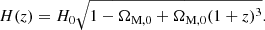
As an additional test, we studied the age–redshift relation assuming a cosmological model directly. In particular, we fitted the median age–redshift with a flat ΛCDM model, where the free parameters are the Hubble constant H0 and the a dimensional matter density parameter (ΩM, 0). Here, we decided to neglect the contribution due to radiation and neutrinos, but we verified that it affects our results by less than 0.2%, which is well below our current error. In this framework, the Hubble parameter H(z) is given by
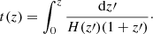
In addition, considering a Friedmann–Lemaitre–Robertson–Walker (FLRW) metric, the age of the Universe at a given redshift t(z) is linked to the Hubble parameter through the following equation:
Before fitting this age–redshift relation to our median data, we needed to pay attention to the fact that t(z) refers to the age of the Universe here, while we obtained ages for a sample of CCs. This means that the two trends are separated by an offset, due to the delay between the Big Bang and the formation of the first galaxies. We parameterised this offset as t0, representing the age of the Universe at which our CCs formed. Assuming that the objects in the sample are coeval, t0 can be considered constant in redshift. Its value will instead be left free to vary. Introducing t0, Eq. (11) can be modified to suit the CCs age–redshift trend as follows:
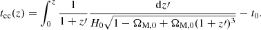
Constraining these three parameters at the same time is a non-trivial process, mainly due to their degeneracies; for example, a higher t0 results in a lower age of the Universe, but this happens with a higher H0 or a larger ΩM, 0 too. As it is also shown in Borghi et al. (2022b), even if these degeneracies are non-negligible, the three parameters affect the age–redshift slope differently. So, if age errors are small enough and if appropriate priors on the parameters are adopted, we could at least partially mitigate these degeneracies.
We performed the fit of the age–redshift relation obtained with binning A (shown in Fig. 7 and described in Table 3) with the theoretical trend in Eq. (12) by adopting a Markov chain Monte Carlo (MCMC) technique implemented through the affine-invariant emcee sampler (Foreman-Mackey et al. 2013) and considering a Gaussian likelihood function. Uniform uninformative priors were assumed for H0 and t0: H0 ∼ 𝒰(25, 125), t0 ∼ 𝒰(0.5, 5). For ΩM, 0, a Gaussian prior is adopted: ΩM, 0 ∼ 𝒢(0.3, 0.02); this is required to keep degeneracies under control. Its value and uncertainty refer to the ones used in Jimenez et al. (2019), resulting from the combination of different measurements of ΩM, 0, all independent of the cosmic microwave background (CMB).
If the mass-downsizing scenario is valid, lower mass galaxies would have formed later than higher-mass ones. Since the median age–redshift relation is divided into a high-mass and a low-mass sample, to take this effect into account, we introduced a parameter #x0394;t that measures the offset in formation time between the two populations. Differently from t0, #x0394;t is not considered a free parameter, but its value is assumed constant and is computed as the average age separation between these two sub-samples. For binning A we find #x0394;t ∼ 0.8 Gyr. To jointly fit all data, therefore, we considered this shift of the lower mass sample in our analysis.
Performing the fit, we obtain  km s−1 Mpc−1 and
  Gyr. Values and errors are, respectively, medians and 1σ values of the posterior distribution. Results are shown in Fig. 9, where grey curves are drawn from the posterior distribution of parameters between 16th and 84th percentiles.
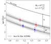 |
Fig. 9. Fit to median age–redshift trend obtained with binning A. Red and blue dots are median values, respectively, for the high-mass (log(Mformed/M⊙) > 11.26) and the low-mass (log(Mformed/M⊙)≤11.26) sample. In grey, we show flat ΛCDM trends with (H0, ΩM, 0, t0) values randomly extracted from the posterior distribution, comprised between 16th and 84th percentiles. Dashed black lines represent the best fit. |
Comparing these results with the ones in Riess et al. (2022) and Planck Collaboration VI (2020), we can say that our errors are not conclusive enough to prefer one or the other, and our measurements agree both with the late- and the early-Universe estimations of H0. We note here that the large error on H0 is mostly due to the very low statistics of CCs available in this analysis. However, these results are still promising in view of upcoming large surveys, such as Euclid (Laureijs et al. 2011), where both the redshift coverage and the much lower statistical errors, granted by the much higher statistics, could significantly increase the precision of the cosmological parameters.
5. Conclusions
In this work, we selected and analysed a sample of massive and passively evolving galaxies from data release 4 of the VANDELS spectroscopic survey (McLure et al. 2018), with the purpose of estimating the Hubble parameter H(z) with the cosmic chronometers method. We adopted a full-spectral-fitting technique to estimate the physical properties of the sample, to benefit from all the spectral and photometric information available in VANDELS, using the code BAGPIPES (Carnall et al. 2018), which was already adopted and optimised within the survey. Differently from the studies already carried out in VANDELS, in this work we adopted a modified version of the code introduced in Jiao et al. (2023), where a non-cosmological prior is assumed on the age of the galaxy population, which is free to vary between 0 and 20 Gyr at all redshifts. This means that the resulting ages are not constrained by a chosen cosmology, but depend only on the adopted stellar population synthesis models and on the component used in the fit to reproduce spectra and photometry.
Our main results are summarised as follows:
-
We selected a sample of 49 purely passive galaxies in the 1 < z < 1.5 redshift range, adopting multiple and complementary selection criteria: a photometric criterion (UVJ), a cut on the [OII] emission line, a cut on the H/K ratio, a visual inspection, and also a redshift cut. The latter is needed because of an anomaly found in the D4000 trend, for which galaxies at z < 1.07 are discarded to avoid biases in the subsequent analysis. The selected galaxies show a red continuum, no emission lines linked to stellar activity, and no H/K inversion. They turn out to have high stellar masses and low sSFR, with median values of ⟨log(M⋆/M⊙)⟩ = 10.88 ± 0.05 and ⟨log(sSFR/yr−1)⟩ = −12.2 ± 0.2.
-
Studying the evolution of age-related spectral features, mainly D4000 and Dn4000, we observe a clear decreasing trend with redshift. Since these features are proven to correlate with the galaxy age, this gives initial, purely observational evidence that the population under analysis is ageing with cosmic time. We also observe that, at fixed redshift, more massive galaxies show a higher D4000 with respect to the lower mass ones, supporting a mass-downsizing scenario.
-
Performing full-spectral-fitting, we obtain age estimates below the age of the Universe in a standard flat ΛCDM model (ΩM = 0.3, ΩΛ = 0.7 and H0 = 70 km s−1 Mpc−1) for 95% of the sample, even if they could formally vary between 0 and 20 Gyr. This proves the robustness of our estimates, where the good quality of VANDELS data allows us to determine correct ages, even without imposing the standard cosmological prior on them. Ages also decrease with redshift, in agreement with this cosmological model, and, at fixed redshift, more massive galaxies result older than lower mass ones, confirming the mass-downsizing trend. The sample is characterised by high masses, sub-solar metallicities, low dust extinction, and a short period of star formation, with median values of mass, metallicity, dust reddening, and τ parameter equal to ⟨log(Mformed/M⊙)⟩ = 11.21 ± 0.05, ⟨Z/Z⊙⟩ = 0.44 ± 0.01, ⟨AV, dust⟩ = 0.43 ± 0.02 mag, and ⟨τ⟩ = 0.28 ± 0.02 Gyr. Metallicity values are compatible with those obtained in Carnall et al. (2022) on a sample of VANDELS passive galaxies.
-
Comparing results obtained by fitting with a delayed SFH or a double-power-law SFH, we find that, despite the different functional forms, the two turn out to be identical if the involved parameters are constrained in a physically reasonable range. In particular, by setting a lower limit to the rising slope of the double-power-law SFH, β > 10, the median percentage difference in age and metallicity estimates is below 2%, for dust reddening and velocity dispersion is less than 1%, while for stellar mass is of 0.001 dex.
-
We further cleaned the 49 galaxies in the sample by removing bad fits and applying a mass cut (log(Mformed/M⊙)≤10.8) to homogenise it, ending with a sample of 39 cosmic chronometers. We built a median age–redshift relation by dividing the sample into two mass bins and two redshift bins. By fitting this median age–redshift relation with a flat ΛCDM model, we obtain an estimate for the Hubble constant
 km s−1 Mpc−1 and for the formation time of high-mass objects of
  Gyr. In doing this, we needed to set a Gaussian prior on ΩM, 0 = 0.30 ± 0.02 in order to keep degeneracies under control.
 -
Finally, we obtain a new, cosmology-independent direct measurement of the Hubble parameter at z ∼ 1.26 equal to H(z) = 135 ± 65 km s−1 Mpc−1 by applying the cosmic chronometers method. Errors include both statistical and systematic uncertainties, with the first dominating the error budget. In the systematic component, we include the effect on the H(z) estimate by using a more complex SFH and the effect of changing the binning while computing the median age–redshift relation.
In conclusion, this work provides additional evidence supporting the robustness of the CC method up to z = 1.5 while proving the effectiveness, even at this redshift, of adopting a full-spectral-fitting approach to extract ages and physical parameters of the galaxy population.
At the same time, the positive results obtained in terms of H(z) and H0, despite the poor statistics, are very promising in view of upcoming large spectroscopic surveys such as Euclid (Laureijs et al. 2011). Forecasting a number of cosmic-chronometer candidates of two orders of magnitude greater than the ones in this work, we could expect to bring down the statistical error to 6% up to z ∼ 2.
Acknowledgments
We thank the anonymous referee for the constructive and useful suggestions that helped in improving this paper. M.M. and A.Cim. acknowledge the grants ASI n.I/023/12/0 and ASI n.2018-23-HH.0. A.Cim. acknowledges the support from grant PRIN MIUR 2017 – 20173ML3WW_001. M.M. acknowledges support from MIUR, PRIN 2017 (grant 20179ZF5KS). E.T. acknowledges the support from COST Action CA21136 – “Addressing observational tensions in cosmology with systematics and fundamental physics (CosmoVerse)”, supported by COST (European Cooperation in Science and Technology). A.C.Car. thanks the Leverhulme Trust for their support via a Leverhulme Early Career Fellowship.
References
- Balogh, M. L., Morris, S. L., Yee, H. K. C., Carlberg, R. G., & Ellingson, E. 1999, ApJ, 527, 54 [Google Scholar]
- Belli, S., Genzel, R., Förster Schreiber, N. M., et al. 2017, ApJ, 841, L6 [NASA ADS] [CrossRef] [Google Scholar]
- Bennett, C. L., Halpern, M., Hinshaw, G., et al. 2003, ApJS, 148, 1 [Google Scholar]
- Borghi, N., Moresco, M., Cimatti, A., et al. 2022a, ApJ, 927, 164 [NASA ADS] [CrossRef] [Google Scholar]
- Borghi, N., Moresco, M., & Cimatti, A. 2022b, ApJ, 928, L4 [NASA ADS] [CrossRef] [Google Scholar]
- Bruzual, G. 1983, ApJ, 273, 105 [CrossRef] [Google Scholar]
- Bruzual, G., & Charlot, S. 2003, MNRAS, 344, 1000 [NASA ADS] [CrossRef] [Google Scholar]
- Buchner, J. 2016, Stat. Comput., 26, 383 [Google Scholar]
- Calabrò, A., Castellano, M., Pentericci, L., et al. 2021, A&A, 646, A39 [EDP Sciences] [Google Scholar]
- Calabrò, A., Pentericci, L., Talia, M., et al. 2022, A&A, 667, A117 [NASA ADS] [CrossRef] [EDP Sciences] [Google Scholar]
- Calzetti, D., Armus, L., Bohlin, R. C., et al. 2000, ApJ, 533, 682 [NASA ADS] [CrossRef] [Google Scholar]
- Cappellari, M. 2017, MNRAS, 466, 798 [Google Scholar]
- Cardelli, J. A., Clayton, G. C., & Mathis, J. S. 1989, ApJ, 345, 245 [Google Scholar]
- Carnall, A. C., McLure, R. J., Dunlop, J. S., & Davé, R. 2018, MNRAS, 480, 4379 [Google Scholar]
- Carnall, A. C., McLure, R. J., Dunlop, J. S., et al. 2019, MNRAS, 490, 417 [Google Scholar]
- Carnall, A. C., McLure, R. J., Dunlop, J. S., et al. 2022, ApJ, 929, 131 [NASA ADS] [CrossRef] [Google Scholar]
- Charlot, S., & Fall, S. M. 2000, ApJ, 539, 718 [Google Scholar]
- Charlot, S., & Longhetti, M. 2001, MNRAS, 323, 887 [NASA ADS] [CrossRef] [Google Scholar]
- Chevallard, J., & Charlot, S. 2016, MNRAS, 462, 1415 [NASA ADS] [CrossRef] [Google Scholar]
- Cid Fernandes, R., Mateus, A., Sodré, L., Stasińska, G., & Gomes, J. M. 2005, MNRAS, 358, 363 [Google Scholar]
- Cimatti, A., & Moresco, M. 2023, ApJ, 953, 149 [NASA ADS] [CrossRef] [Google Scholar]
- Citro, A., Pozzetti, L., Quai, S., et al. 2017, MNRAS, 469, 3108 [Google Scholar]
- Conroy, C., Graves, G. J., & van Dokkum, P. G. 2014, ApJ, 780, 33 [Google Scholar]
- Cullen, F., McLure, R. J., Dunlop, J. S., et al. 2019, MNRAS, 487, 2038 [Google Scholar]
- Cullen, F., McLure, R. J., Dunlop, J. S., et al. 2020, MNRAS, 495, 1501 [Google Scholar]
- Eisenstein, D. J., Zehavi, I., Hogg, D. W., et al. 2005, ApJ, 633, 560 [Google Scholar]
- Estrada-Carpenter, V., Papovich, C., Momcheva, I., et al. 2019, ApJ, 870, 133 [NASA ADS] [CrossRef] [Google Scholar]
- Ferland, G. J., Chatzikos, M., Guzmán, F., et al. 2017, Rev. Mex. Astron. Astrofis., 53, 385 [NASA ADS] [Google Scholar]
- Foreman-Mackey, D., Hogg, D. W., Lang, D., & Goodman, J. 2013, PASP, 125, 306 [Google Scholar]
- Franzetti, P., Scodeggio, M., Garilli, B., et al. 2007, A&A, 465, 711 [NASA ADS] [CrossRef] [EDP Sciences] [Google Scholar]
- Garilli, B., McLure, R., Pentericci, L., et al. 2021, A&A, 647, A150 [NASA ADS] [CrossRef] [EDP Sciences] [Google Scholar]
- Gavazzi, G., Bonfanti, C., Sanvito, G., Boselli, A., & Scodeggio, M. 2002, ApJ, 576, 135 [NASA ADS] [CrossRef] [Google Scholar]
- Giavalisco, M., Ferguson, H. C., Koekemoer, A. M., et al. 2004, ApJ, 600, L93 [NASA ADS] [CrossRef] [Google Scholar]
- Grogin, N. A., Kocevski, D. D., Faber, S. M., et al. 2011, ApJS, 197, 35 [NASA ADS] [CrossRef] [Google Scholar]
- Guaita, L., Pompei, E., Castellano, M., et al. 2020, A&A, 640, A107 [NASA ADS] [CrossRef] [EDP Sciences] [Google Scholar]
- Hamadouche, M. L., Carnall, A. C., McLure, R. J., et al. 2022, MNRAS, 512, 1262 [NASA ADS] [CrossRef] [Google Scholar]
- Hoag, A., Treu, T., Pentericci, L., et al. 2019, MNRAS, 488, 706 [Google Scholar]
- Ilbert, O., Salvato, M., Le Floc’h, E., et al. 2010, ApJ, 709, 644 [Google Scholar]
- Ilbert, O., McCracken, H. J., Le Fèvre, O., et al. 2013, A&A, 556, A55 [NASA ADS] [CrossRef] [EDP Sciences] [Google Scholar]
- Jiao, K., Borghi, N., Moresco, M., & Zhang, T.-J. 2023, ApJS, 265, 48 [NASA ADS] [CrossRef] [Google Scholar]
- Jimenez, R., & Loeb, A. 2002, ApJ, 573, 37 [NASA ADS] [CrossRef] [Google Scholar]
- Jimenez, R., Cimatti, A., Verde, L., Moresco, M., & Wandelt, B. 2019, JCAP, 2019, 043 [CrossRef] [Google Scholar]
- Kamionkowski, M., & Riess, A. G. 2023, Annu. Rev. Nucl. Part. Sci., 73, 153 [NASA ADS] [CrossRef] [Google Scholar]
- Koekemoer, A. M., Faber, S. M., Ferguson, H. C., et al. 2011, ApJS, 197, 36 [NASA ADS] [CrossRef] [Google Scholar]
- Kriek, M., Price, S. H., Conroy, C., et al. 2019, ApJ, 880, L31 [NASA ADS] [CrossRef] [Google Scholar]
- Kroupa, P. 2001, MNRAS, 322, 231 [NASA ADS] [CrossRef] [Google Scholar]
- Laureijs, R., Amiaux, J., Arduini, S., et al. 2011, ArXiv e-prints [arXiv:1110.3193] [Google Scholar]
- Lonoce, I., Maraston, C., Thomas, D., et al. 2020, MNRAS, 492, 326 [NASA ADS] [CrossRef] [Google Scholar]
- Luo, B., Brandt, W. N., Xue, Y. Q., et al. 2017, ApJS, 228, 2 [Google Scholar]
- Magliocchetti, M., Pentericci, L., Cirasuolo, M., et al. 2020, MNRAS, 493, 3838 [Google Scholar]
- Magris, G., Binette, L., & Bruzual, G. 2003, ApJS, 149, 313 [CrossRef] [Google Scholar]
- Marchi, F., Pentericci, L., Guaita, L., et al. 2019, A&A, 631, A19 [NASA ADS] [CrossRef] [EDP Sciences] [Google Scholar]
- McLure, R. J., Pentericci, L., Cimatti, A., et al. 2018, MNRAS, 479, 25 [NASA ADS] [Google Scholar]
- Mignoli, M., Zamorani, G., Scodeggio, M., et al. 2009, A&A, 493, 39 [NASA ADS] [CrossRef] [EDP Sciences] [Google Scholar]
- Moresco, M. 2023, ArXiv e-prints [arXiv:2307.09501] [Google Scholar]
- Moresco, M., Jimenez, R., Cimatti, A., & Pozzetti, L. 2011, JCAP, 2011, 045 [CrossRef] [Google Scholar]
- Moresco, M., Cimatti, A., Jimenez, R., et al. 2012, JCAP, 2012, 006 [CrossRef] [Google Scholar]
- Moresco, M., Pozzetti, L., Cimatti, A., et al. 2013, A&A, 558, A61 [NASA ADS] [CrossRef] [EDP Sciences] [Google Scholar]
- Moresco, M., Jimenez, R., Verde, L., et al. 2018, ApJ, 868, 84 [NASA ADS] [CrossRef] [Google Scholar]
- Moresco, M., Amati, L., Amendola, L., et al. 2022, Liv. Rev. Relat., 25, 6 [NASA ADS] [Google Scholar]
- Onodera, M., Carollo, C. M., Renzini, A., et al. 2015, ApJ, 808, 161 [NASA ADS] [CrossRef] [Google Scholar]
- Pentericci, L., McLure, R. J., Garilli, B., et al. 2018, A&A, 616, A174 [NASA ADS] [CrossRef] [EDP Sciences] [Google Scholar]
- Percival, W. J., Baugh, C. M., Bland-Hawthorn, J., et al. 2001, MNRAS, 327, 1297 [Google Scholar]
- Perlmutter, S., Aldering, G., Goldhaber, G., et al. 1999, ApJ, 517, 565 [Google Scholar]
- Planck Collaboration VI. 2020, A&A, 641, A6 [NASA ADS] [CrossRef] [EDP Sciences] [Google Scholar]
- Pozzetti, L., Bolzonella, M., Zucca, E., et al. 2010, A&A, 523, A13 [NASA ADS] [CrossRef] [EDP Sciences] [Google Scholar]
- Riess, A. G., Filippenko, A. V., Challis, P., et al. 1998, AJ, 116, 1009 [Google Scholar]
- Riess, A. G., Yuan, W., Macri, L. M., et al. 2022, ApJ, 934, L7 [NASA ADS] [CrossRef] [Google Scholar]
- Rose, J. A. 1984, AJ, 89, 1238 [NASA ADS] [CrossRef] [Google Scholar]
- Salim, S., Boquien, M., & Lee, J. C. 2018, ApJ, 859, 11 [Google Scholar]
- Saracco, P., Barbera, F. L., De Propris, R., et al. 2023, MNRAS, 520, 3027 [NASA ADS] [CrossRef] [Google Scholar]
- Saxena, A., Pentericci, L., Mirabelli, M., et al. 2020a, A&A, 636, A47 [NASA ADS] [CrossRef] [EDP Sciences] [Google Scholar]
- Saxena, A., Pentericci, L., Schaerer, D., et al. 2020b, MNRAS, 496, 3796 [Google Scholar]
- Schreiber, C., Glazebrook, K., Nanayakkara, T., et al. 2018, A&A, 618, A85 [NASA ADS] [CrossRef] [EDP Sciences] [Google Scholar]
- Straatman, C. M. S., van der Wel, A., Bezanson, R., et al. 2018, ApJS, 239, 27 [NASA ADS] [CrossRef] [Google Scholar]
- Talia, M., Schreiber, C., Garilli, B., et al. 2023, A&A, 678, A25 [NASA ADS] [CrossRef] [EDP Sciences] [Google Scholar]
- Thomas, D., Maraston, C., Schawinski, K., Sarzi, M., & Silk, J. 2010, MNRAS, 404, 1775 [NASA ADS] [Google Scholar]
- Thomas, D., Maraston, C., & Johansson, J. 2011, MNRAS, 412, 2183 [Google Scholar]
- Thomas, R., Pentericci, L., Le Fevre, O., et al. 2020, A&A, 634, A110 [NASA ADS] [CrossRef] [EDP Sciences] [Google Scholar]
- Thomas, R., Pentericci, L., Le Fèvre, O., et al. 2021, A&A, 650, A63 [NASA ADS] [CrossRef] [EDP Sciences] [Google Scholar]
- Valcin, D., Jimenez, R., Verde, L., Bernal, J. L., & Wandelt, B. D. 2021, JCAP, 2021, 017 [CrossRef] [Google Scholar]
- Williams, R. J., Quadri, R. F., Franx, M., van Dokkum, P., & Labbé, I. 2009, ApJ, 691, 1879 [NASA ADS] [CrossRef] [Google Scholar]
Appendix A: The z< 1.07 anomaly
The discontinuity at 4000 Å, known as D4000 break, is a spectral feature tightly connected to the age (and metallicity) of passive galaxies. For a homogeneous population where the evolution in metallicity is negligible, we expect a decreasing trend with redshift for this quantity (Moresco et al. 2012), as also shown by theoretical models reported in Fig. A.1. In the redshift range of 1< z< 1.07, highlighted in Fig. A.1 with a shaded region, we instead find an anomalous behaviour: all the objects in this redshift bin show a much weaker Dn4000 than expected, comparable to the values obtained at z = 1.3-1.4, independently of stellar mass. In order to understand the origin of this anomaly, we explored different hypotheses.
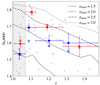 |
Fig. A.1. Dn4000 trend with redshift. In grey, we show the measurements for the single objects of the CCs sample; blue and red dots are median values for objects with log(M⋆/M⊙)≤10.86 (high-mass) and log(M⋆/M⊙) > 10.86 (low-mass), respectively; similarly, blue and red stars are measurements obtained on stacked spectra of low- and high-mass samples. In the background, lines refer to evolutionary models from Bruzual & Charlot (2003) at different formation redshifts. |
The first possible origin that we considered is that some errors in the D4000 measurements were made. To check this, we produced eight stacked spectra, one for each red or blue point in Fig. A.1, first dividing the sample into a high-mass and a low-mass sample with respect to the median mass (log(Mformed/M⊙) = 10.86), and then in four redshift bins. In this way, we were able to obtain spectra with a higher S/N and, therefore, reduce the possibility of a measurement error. We also normalised the eight stacked spectra to their median value in the 3850–3950 Å range, which is the blue wavelength range used in computing Dn4000. We chose this window because in normalising the spectra in this interval we were able to visually check in the red band of the Dn4000 eventual differences among the different spectra. The four stacked spectra for the high-mass sample are shown in Fig. A.2. The coloured horizontal lines at 4000 < λ < 4100 Å represent the average flux in the red window of the Dn4000, and since the spectra have all been normalised in the blue window, they allow us to check differences in the Dn4000, which is the ratio between the average fluxes in these intervals, by eye. As it is possible to see, the average flux at z∼1.04 (blue line) is almost equal to the average flux at z∼1.34 (red line), while at the other redshifts the behaviour is as expected. We observe the same pattern for the low-mass stacked spectra. This means that the population of galaxies in the lowest redshift bin, where we find the anomaly, does effectively show a lower Dn4000 than expected, similar to the one obtained in the highest redshift bin. For this reason, we reject the hypothesis of a measurement error.
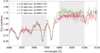 |
Fig. A.2. Median stacked spectra obtained for the high-mass sample in each of the four redshift bins, normalised to their mean value in the blue band of the Dn4000. In grey, we show the two windows in which the red and blue bands of the Dn4000 are defined, while horizontal lines represent their median values in these two ranges. We remind the reader that the median spectra have been normalised in the blue window; therefore, the average fluxes of the four spectra in that region are identical by definition. |
Since this drop in D4000 appears for galaxies at z< 1.07, we considered the possibility of calibration issues. In fact, it involves all the objects in a specific redshift interval and regards mainly ‘wide’ spectroscopic features (such as Dn4000 and Mgwide, while we do not see this anomaly for spectral indices that concern #x0394;λ ≲ 200 Å), so a calibration effect seems plausible. In order to observe this type of behaviour in the D4000, the hypothetical calibration should have increased the observed flux bluer than 8300 Å by ∼10% or, equivalently, decreased it by ∼10% at wavelength redder than 8300 Å, where the D4000 is observed at this redshift. As explained in Garilli et al. (2021), a blue-end correction was indeed applied to the spectra, but it is of the order of 5% and significant only at λ ≲ 5500 Å (observed-frame), and thus not able to justify the observed anomaly. The issue was reported to the VANDELS collaboration, but no other calibration effect was pointed out. Therefore, a calibration issue can be excluded as the anomaly’s source.
Up to now we know that the D4000 drop is actually present in the spectra and that it is not related to a measurement issue, so we wish to explore the possibility of it being related to a real effect concerning galaxy properties. A lower D4000 in a passive galaxy could mean a younger age, a lower metallicity, or a lower dust extinction; even if this were the case, we should still find a reason for these properties characterising this particular redshift bin. We analysed the available physical properties of the sample, this time splitting it into the two fields of observation, CDFS and UDS, so that possible anomalies concerning one of the two fields could be pointed out. Looking at the trends in stellar mass, sSFR, and dust extinction, we do not find substantial differences either throughout redshift or among fields. If we instead consider the age as a trigger, we have two possibilities: the first is that this group of galaxies underwent rejuvenation processes, maybe due to an environmental effect; the second is that an unexpected selection effect is present.
Looking for an environmental difference in the population at z< 1.07, we investigated the presence of overdensities in this redshift interval. Studying the redshift distribution of the sample, we observe that both in UDS and CDFS an overdensity is present around z∼1.04. A dense environment can in fact be a reason for rejuvenation if, for example, it triggers intense merger phenomena. Anyway, this should happen equally in both fields to justify the effect in our data, since the D4000 drop is of the same entity in CDFS and UDS. Moreover, we see that the overdensity at z∼1.04 is not the only one, but others are present at higher redshift. At z∼1.09 in UDS, for example, an important overdensity is present, but we do not see any anomaly in this redshift bin. Hence, the rejuvenation hypothesis seems unlikely.
The second option of a possible selection effect was presented to the VANDELS collaboration, but again nothing was found to justify the anomaly. Upon further scrutiny, we noticed that at z< 1.07 a higher fraction of objects is provided with just ground-based photometry with respect to the z> 1.07 sample, in particular in the CDFS field. This does not explain, per se, the anomaly, but it could hint at the possible origin if a selection effect is present in the preparation of the ground-based catalogues.
Whatever the cause, in order to avoid any potential bias in our cosmological analysis, we decided to remove the galaxies at z< 1.07 from our sample. We emphasise that this simply reduces the statistics of the sample, it does not affect the robustness of the cosmological results.
Finally, we also tested how the results would change by changing the threshold cut in redshift, setting it to lower values (e.g. 1.05, 1.04). By doing so, we verified that including even a few of these anomalous objects would strongly bias the determination of the Hubble parameter. Due to their low D4000, all the galaxies below z = 1.07 appear younger, affecting the slope of age-z by making it significantly shallower with respect to the homogeneous trend observed at z> 1.07, and, in turn, producing a higher H(z).
Appendix B: Assessing the impact of the SFH choice
The SFH choice is certainly one of the most significant components when building a fitting model since it describes how the star-formation rate varies as a function of cosmic time and then dictates the chemical enrichment history of the galaxy, as well as its stellar mass. As discussed in Sect. 3.1, the DPL SFH is a valid alternative to the DED SFH that we use as baseline, and it has actually already been adopted while analysing VANDELS data (Carnall et al. 2019, 2022). There are two main differences with respect to a DED SFH: the first is that a DPL has three free parameters instead of two since its shape is determined separately by the falling (α) and the rising slope (β) of the curve; the second regards the definition of the galaxy age, which is, by default in BAGPIPES, the mass-weighted quantity defined in Eq. 7 instead of the one in Eq. 6 adopted for a DED SFH. For the sake of consistency, in this section we use mass-weighted ages for both DED and DPL SFH assumptions.
As presented in Sect. 3.2, we performed a fit adopting a DPL SFH named configuration 1, with parameters and priors as listed in Tab. 2. Once we remove the bad fits, we find an exceptional agreement with baseline results for 75% of the galaxy population, as shown in Fig. B.1, with a median percentage difference in terms of mass-weighted age, stellar mass, metallicity, dust reddening, and velocity dispersion smaller than 1%. The rest of the sample (six objects) shows a significant difference with respect to baseline results (purple open dots in Fig. B.1).
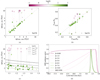 |
Fig. B.1. Comparison of physical parameters obtained with delayed exponentially declining (DED) and double-power-law (DPL) SFH. In panels (a) and (b) we show the comparison of mass-weighted ages and metallicities estimated with the two SFHs. The points are colour-coded according to the parameter β of the DPL model, representing the rising slope of the SFH. We notice that the objects with extremely low β (represented with open circles) are the ones deviating more from the one-to-one relation. For this reason, we fitted those objects again with a more conservative prior on β (β > 10). The grey arrows show how the results converge to the correct relation with the new prior. In panel (c) we present the age-redshift relation with the same colour-coding as in the previous panels. In panel (d) the star-formation rate is shown as a function of the look-back time normalised to its peak for an object significantly deviating from the one-to-one relation in panel (a). The coloured curves represent how the resulting SFH obtained with the DPL model changes with different priors on β, colour-coded as presented in the legend; the grey dashed line shows the DED SFH, for comparison. We notice that above β > 6 the DPL model converges almost exactly to the DED model. |
To understand the nature of this difference, we examined all the properties of these six CCs, finding that they show common characteristics, in particular ages over 5 Gyr and β < 1. Recalling that β sets the rising slope of the SFH, a value β < 1 implies that the first part of the SFH has a concave shape, as in the dark purple curve in Fig. B.1d, causing an extremely slow rise of the SFR. Solutions of this kind appear highly non-physical because they would require a SFH extremely prolonged over time and without significant episodes of star formation, in contradiction with other indicators available (e.g. the measured sSFR, H/K ratio, etc.) and with all the other results obtained in the literature for these extremely massive and passive systems. For the population whose results agree with baseline ones, instead, the value of β spans from a few tens to hundreds, resulting in a very steep rise of the SFR. It seems that relaxing the cosmological prior on ages and adopting a DPL SFH, which is more flexible than a DED SFH in terms of shape, in some cases allows the fit to find a combination of parameters leading to a non-physical solution.
We ran some tests to understand if a different, physically acceptable solution exists for these objects by increasing the prior on β. In Fig. B.1d, we show the SFHs obtained for an example object resulting from seven runs where the β prior was gradually raised from 0.001 to 10. We can observe that up to β > 5 the resulting SFH still has an anomalous shape and duration, with values for β near the prior limit, suggesting that the fit is still trying to reach the non-physical solution. From prior β > 6 on, we instead find solutions with values for β two orders of magnitude larger, and, above this limit, in all cases increasing the value of the prior leads to the exact same solution, which is also almost identical to the SFH found when fitting with a DED SFH. This means that a physical solution for these objects does exist, and, if the SFH parameters are properly constrained, the resulting SFH has the same shape if either a DED SFH or a DPL SFH is assumed.
Based on these findings, we repeated the fit on all of our 49 objects using configuration 1 (Tab. 2), this time increasing the lower limit on β to 10. In Figs. B.1a and B.1b we show the comparison of results for mass-weighted ages and metallicity between baseline (x-axis) and configuration 1 (y-axis) both with the old (open dots) and the new prior (full dots). It is clear that after applying the new prior the results of the two fits have a one-to-one correlation, with a median percentage difference lower than 2% for both quantities. In terms of stellar mass, velocity dispersion, and dust reddening, the discrepancy is even smaller, reaching a median percent difference lower than 1%. Given the colour-code applied in these figures, it is also evident how the results of configuration 1 with the old prior are different from the ones obtained with the new prior only when β converges to values lower than 1, while in all the other cases they overlap almost perfectly. The same behaviour is noticeable in the age-redshift relation shown in Fig. B.1c.
We can conclude that the impact of the SFH choice on the estimation of physical parameters is minimal, under the condition that the SFH parameters are constrained to avoid non-physical solutions. In particular, a lower limit to the rising slope of the DPL SFH β > 10 is effective for this purpose. In addition, the fact that the resulting SFH shape is equivalent when adopting a DED or a DPL SFH further validates the robustness of results obtained with the baseline configuration, despite the existent degeneracy between age and τ in a DEL SFH discussed in Sect. 3.3.
In addition to these tests, we also used configuration 1 results to estimate a value of the Hubble parameter with the DPL SFH, finding very good agreement with the results obtained with the DED SFH. This demonstrates that not only are the absolute ages obtained assuming different SFH in very good agreement, the relative ages are too, proving the robustness of the CC method against the assumption of a specific SFH model (due to the strictness and purity of our selection of CC candidates).
All Tables
Parameters and priors adopted for each configuration used in the full spectrum fitting.
Median ages and properties of the selected CC sample considering the binning A as described in the text.
Measurements of H(z) obtained applying the CC method to median age–redshift trends obtained with baseline and configuration 1 fits, both using binning A and binning B.
All Figures
|
Fig. 1. Histograms for the physical and spectral properties of the samples in each selection step, as shown in the legend and described in Sect. 2.2. Vertical arrows represent the corresponding median values, and, when present, the dashed vertical line indicates the threshold value adopted to select cosmic chronometers according to that quantity (the shaded area showing the discarded range). We note that for the [OII] we adopted a conservative cut, discarding only the objects that showed both EW([OII]) > 5 Å and S/N([OII]) > 3, aiming to keep objects in which the [OII] line could be due to noise fluctuation. |
| In the text | |
|
Fig. 2. Photometric and spectroscopic selection criteria. Top: UVJ diagram for the main selection steps. Galaxies above the dashed line are qualified as passive following the criterion in McLure et al. (2018). Bottom: EW[OII] versus H/K ratio, colour-coded by S/N[OII], for the sample after the UVJ cut. The shaded areas show the discarded ranges for both quantities. |
| In the text | |
|
Fig. 3. Median stacked spectra estimated for the different incremental selected samples of our analysis, as described in Sect. 2.2. We underline that the final sample considered is the purple one, on which we also highlight the most characteristic absorption features (grey shaded area) and spectral breaks (dashed area), as well as the position of potential emission lines (red shaded area), showing the absence of emission lines in our final sample. |
| In the text | |
|
Fig. 4. Dn4000 trend with redshift. The measurements for the single objects of the CCs sample are shown in grey; blue and red dots are median values averaged in two mass bins, log(M⋆/M⊙)≤10.88 (high-mass) and log(M⋆/M⊙) > 10.88 (low-mass), respectively. The different lines show the Dn4000–z relation obtained from the 2016 version of the Bruzual & Charlot (2003) models at different formation redshifts and assuming a reference flat ΛCDM cosmology (ΩM = 0.3, ΩΛ = 0.7 and H0 = 70 km s−1 Mpc−1), purely for illustrative purposes. We note that, qualitatively, the observed trends follow the cosmological models quite well, but we defer to Sect. 4 the full cosmological analysis. |
| In the text | |
|
Fig. 5. Example of best-fit spectrum and photometry (in orange) obtained by fitting the observed ones (in blue) with the baseline configuration, as described in Sect. 3.2. |
| In the text | |
|
Fig. 6. Trends with redshift of age (a), stellar mass (b), tau parameter (c), and metallicity (d), colour-coded by stellar mass. In the age–redshift the lines in the background represent the theoretical trends in a flat ΛCDM cosmology with ΩM, 0 = 0.3, ΩΛ, 0 = 0.7, H0 = 70 km s−1 Mpc−1, and different formation redshifts. |
| In the text | |
|
Fig. 7. Median age–redshift trend for the 39 CCs sample, obtained with binning A. Red and blue dots represent median values, respectively, for the high-mass (log(Mformed/M⊙) > 11.26) and the low-mass (log(Mformed/M⊙)≤11.26) sample. In the background, grey dots are the 39 single measurements, while lines show, for illustrative purposes only, the theoretical trends with different redshifts of formation, as given by a flat ΛCDM model with ΩM = 0.3, ΩΛ = 0.7 and H0 = 70 km s−1 Mpc−1. |
| In the text | |
|
Fig. 8. H(z) measurement obtained in this work in comparison with all the H(z) estimations obtained up to now with the cosmic chronometers method. The dashed line represents the theoretical trend of a flat ΛCDM model as in Planck Collaboration VI (2020) as a purely illustrative reference. |
| In the text | |
|
Fig. 9. Fit to median age–redshift trend obtained with binning A. Red and blue dots are median values, respectively, for the high-mass (log(Mformed/M⊙) > 11.26) and the low-mass (log(Mformed/M⊙)≤11.26) sample. In grey, we show flat ΛCDM trends with (H0, ΩM, 0, t0) values randomly extracted from the posterior distribution, comprised between 16th and 84th percentiles. Dashed black lines represent the best fit. |
| In the text | |
|
Fig. A.1. Dn4000 trend with redshift. In grey, we show the measurements for the single objects of the CCs sample; blue and red dots are median values for objects with log(M⋆/M⊙)≤10.86 (high-mass) and log(M⋆/M⊙) > 10.86 (low-mass), respectively; similarly, blue and red stars are measurements obtained on stacked spectra of low- and high-mass samples. In the background, lines refer to evolutionary models from Bruzual & Charlot (2003) at different formation redshifts. |
| In the text | |
|
Fig. A.2. Median stacked spectra obtained for the high-mass sample in each of the four redshift bins, normalised to their mean value in the blue band of the Dn4000. In grey, we show the two windows in which the red and blue bands of the Dn4000 are defined, while horizontal lines represent their median values in these two ranges. We remind the reader that the median spectra have been normalised in the blue window; therefore, the average fluxes of the four spectra in that region are identical by definition. |
| In the text | |
|
Fig. B.1. Comparison of physical parameters obtained with delayed exponentially declining (DED) and double-power-law (DPL) SFH. In panels (a) and (b) we show the comparison of mass-weighted ages and metallicities estimated with the two SFHs. The points are colour-coded according to the parameter β of the DPL model, representing the rising slope of the SFH. We notice that the objects with extremely low β (represented with open circles) are the ones deviating more from the one-to-one relation. For this reason, we fitted those objects again with a more conservative prior on β (β > 10). The grey arrows show how the results converge to the correct relation with the new prior. In panel (c) we present the age-redshift relation with the same colour-coding as in the previous panels. In panel (d) the star-formation rate is shown as a function of the look-back time normalised to its peak for an object significantly deviating from the one-to-one relation in panel (a). The coloured curves represent how the resulting SFH obtained with the DPL model changes with different priors on β, colour-coded as presented in the legend; the grey dashed line shows the DED SFH, for comparison. We notice that above β > 6 the DPL model converges almost exactly to the DED model. |
| In the text | |
Current usage metrics show cumulative count of Article Views (full-text article views including HTML views, PDF and ePub downloads, according to the available data) and Abstracts Views on Vision4Press platform.
Data correspond to usage on the plateform after 2015. The current usage metrics is available 48-96 hours after online publication and is updated daily on week days.
Initial download of the metrics may take a while.