| Issue |
A&A
Volume 696, April 2025
|
|
|---|---|---|
| Article Number | A98 | |
| Number of page(s) | 16 | |
| Section | Cosmology (including clusters of galaxies) | |
| DOI | https://doi.org/10.1051/0004-6361/202452812 | |
| Published online | 08 April 2025 | |
Globular clusters as cosmic clocks: New cosmological hints from their integrated light
1
Dipartimento di Fisica e Astronomia “Augusto Righi”–Università di Bologna, Via Piero Gobetti 93/2, I-40129 Bologna, Italy
2
INAF – Osservatorio di Astrofisica e Scienza dello Spazio di Bologna, Via Piero Gobetti 93/3, I-40129 Bologna, Italy
3
INAF – Osservatorio Astrofisico di Arcetri, Largo E. Fermi 5, I-50125 Firenze, Italy
4
ICC, University of Barcelona, Martí i Franquès, 1, E08028 Barcelona, Spain
5
ICREA, Pg. Lluis Companys 23, Barcelona 08010, Spain
⋆ Corresponding author; This email address is being protected from spambots. You need JavaScript enabled to view it.
Received:
30
October
2024
Accepted:
10
February
2025
Abstract
Aims. In this work, we explore the reliability and robustness in measuring the ages and main physical properties of a sample of old Milky Way globular clusters (GCs) from their integrated light. This approach sets the stage for using GCs as cosmic clocks at high redshift. Additionally, it enables us to establish an independent lower limit on the age of the Universe, and an upper limit on H0.
Methods. We analysed a sample of 77 GCs from the WAGGS project, by first measuring their spectral features (Lick indices and spectroscopic breaks) with PyLick and then performing full spectral fitting with BAGPIPES. The analysis of Lick indices offers an initial estimate of the population’s age and metallicity, generally aligning well with values reported in the literature. However, it also highlights a subset of old clusters for which we estimate younger ages. This discrepancy is primarily attributed to the presence of horizontal branches (HBs) with complex morphologies, which are not accounted for in the stellar population models. With full spectral fitting we measured the GCs’ ages, metallicities, and masses, testing how removing the cosmological prior on the ages affects the final results.
Results. Compared to isochrone fitting estimates, ages are best recovered when the cosmological prior is removed, with a 20% increase in the number of GCs showing ages compatible with literature values within ±1.5 Gyr. The derived metallicity and mass are consistently in good agreement with the reference values, regardless of HB morphology, [Z/H], or the fit settings. The average discrepancies across the entire sample are ⟨Δ[Z/H]⟩ = −0.02 ± 0.24 dex for metallicity and ⟨Δlog(M⋆/M⊙)⟩ = 0.04 ± 0.28 dex for mass. Metal-rich GCs ([Z/H] ≥ −0.4) showing a red HB (with morphological parameter HBR > 0) are the sub-group in which ages are best recovered. In this group, 70% of the results align with literature values within ±1.5 Gyr. Identifying the tail of the oldest cosmology-independent ages with a Gaussian mixture model, we obtained a sample of 24 objects with ⟨age⟩ = 13.4 ± 1.1 Gyr.
Conclusions. Being a natural lower limit on the age of the Universe, we used the age of the oldest GCs to constrain the Hubble constant, obtaining H0 = 70.5−6.3+7.7 km s−1 Mpc−1 (stat+syst) when a flat ΛCDM with Ωm = 0.30 ± 0.02 (based on low-z measurements) was assumed. Validating the analysis of GCs based on their integrated light lays the foundation for extending this type of study to high redshift, where GCs have begun to appear in lensed fields, thanks to JWST.
Key words: globular clusters: general / cosmological parameters / cosmology: observations
© The Authors 2025
 Open Access article, published by EDP Sciences, under the terms of the Creative Commons Attribution License (https://creativecommons.org/licenses/by/4.0), which permits unrestricted use, distribution, and reproduction in any medium, provided the original work is properly cited.
This article is published in open access under the Subscribe to Open model. This email address is being protected from spambots. You need JavaScript enabled to view it. to support open access publication.
1. Introduction
Over the last few decades, the flat ΛCDM model has been a fundamental pillar in cosmology thanks to the support of independent cosmological probes, including the cosmic microwave background (CMB; e.g. Bennett et al. 2003; Planck Collaboration VI 2020), type Ia supernovae (e.g. Riess et al. 1998; Perlmutter et al. 1999), and baryon acoustic oscillations (e.g. Percival et al. 2001; Eisenstein et al. 2005). Nonetheless, further investigation is necessary to unveil the nature of dark matter and dark energy and assess the precise values of cosmological parameters. In fact, due to the higher precision achieved in late- and early-Universe probes, some inconsistencies have emerged regarding the value of the Hubble constant (H0), where a tension of 4–5σ has now been observed (Abdalla et al. 2022).
In this context, the age of the Universe (tU) can play a crucial role, given its sensitivity to H0. Indeed, in a flat ΛCDM cosmology with ΩM = 0.3 and ΩΛ = 0.7, tU can span a range from ∼14.1 Gyr if H0 = 67 km s−1 Mpc−1 to ∼12.9 Gyr if H0 = 73 km s−1 Mpc−1. Thus, measuring the absolute ages of the most long-lived objects at z = 0 can be critical, since they naturally place a lower limit on the current age of the Universe (tU) and, in turn, an upper limit on H0. This provides independent constraints on the Hubble constant and valuable information for investigating the origin of the observed tension.
Globular clusters (GCs) are among the oldest objects in the Universe for which we can accurately determine the age (VandenBerg et al. 1996; Soderblom 2010; Brown et al. 2018; Oliveira et al. 2020; Massari et al. 2023). Composed of roughly one million stars that formed simultaneously with similar composition (though see reviews by Bastian & Lardo 2018; Gratton et al. 2019; Milone & Marino 2022, for discussions on the multiple population phenomenon in massive clusters), these clusters have remained gravitationally bound for up to a Hubble time. Currently, various GC formation models estimate formation redshifts ranging from 5–7 to as high as 10–12 (Valenzuela et al. 2025). Each GC thus serves as an observable record of the age, metallicity, and kinematics from the time of its formation. Therefore, by measuring their ages, we can use them as ‘clocks’ that began ticking in the early stages of the Universe’s evolution (O’Malley et al. 2017; Jimenez et al. 2019; Valcin et al. 2020, 2021; Cimatti & Moresco 2023).
The most straightforward method to determine the age of a GC is to exploit the fact that the position of the main-sequence turn-off (MSTO) in the plane of effective temperature (Teff) versus luminosity (L) changes with age (or mass). Isochrones, or theoretical tracks of stars with the same chemical composition, are fitted to the MSTO region of colour–magnitude diagrams (CMDs) to estimate the age. Even if this is a well-established and robust method, it is important to explore new and complementary approaches that can address the case when the CMD is not available. In need of a spatially resolved stellar population, indeed, isochrone fitting can be applied only to nearby systems, while moving further than the Magellanic Clouds becomes either very expensive in terms of exposure time or even impossible1. Moreover, recent JWST observations of lensed fields highlighted the presence of GC candidates around lensed galaxies, like the Sparkler (Mowla et al. 2022) at z = 1.38, which, if confirmed with spectroscopy, would extend the study of GCs at high redshift. To do so, we need to explore methods relying on GCs’ integrated light and validate them against the traditional methods. In this scenario, one of the best ways to leverage all the integrated light information is to perform full spectral fitting (FSF), a technique that enables one to measure, alongside the age, all the physical properties of the GC such as metallicity, mass, and dust reddening.
Previous works have derived physical parameters of GCs like age and metallicity using the integrated light provided by Schiavon et al. (2005) for 41 Milky Way (MW) GCs (e.g. Koleva et al. 2008; Cezario et al. 2013; Cabrera-Ziri & Conroy 2022), testing different algorithms, like STECKMAP (Ocvirk et al. 2006), NBURSTS (Chilingarian et al. 2007), ULySS (Koleva et al. 2009), or ALF (Conroy & van Dokkum 2012), and different simple stellar population (SSP) models (Bruzual & Charlot 2003; Prugniel & Soubiran 2004; Vazdekis et al. 2010, 2015). Others have benefited from the larger spectral coverage and higher resolution of the WiFeS Atlas of Galactic Globular cluster Spectra project (WAGGS, Usher et al. 2017, 2019a), providing integrated spectra for 113 GCs in the MW and its satellite galaxies (Usher et al. 2019b; Gonçalves et al. 2020; Cabrera-Ziri & Conroy 2022). In Gonçalves et al. (2020), for instance, the authors adopted the non-parametric FSF code STARLIGHT (Cid Fernandes et al. 2005), relying on MILES SSP models (Vazdekis et al. 2015), with a focus on how the wavelength range influences the recovery of the stellar parameters compared to the CMD fitting. Cabrera-Ziri & Conroy (2022) extended the MW GCs sample from Schiavon et al. (2005) by including younger objects from the Large and Small Magellanic Clouds (LMC and SMC) with WAGGS spectra, adopting the non-parametric FSF code ALF. While there is broad agreement that the ages of younger GCs can be reliably determined through FSF, these studies highlighted the challenges in dating the oldest GCs from their integrated spectra, often yielding results significantly younger than those from isochrone-fitting methods.
In this paper, we focus on the oldest tail of the WAGGS GCs, analysing 82 GCs in the MW. We take advantage of the high-quality integrated spectra provided by WAGGS, along with the wealth of data available for these objects, the independent age estimates derived with different techniques, and the fact that GCs are among the simplest stellar systems in the Universe, the closest templates to an SSP we have. We adopt a parametric FSF method, enabling the reconstruction of GCs’ integrated emission within a high-dimensional parameter space. For this purpose, we use the FSF code BAGPIPES (Carnall et al. 2018) utilising the 2016 version of the Bruzual & Charlot (2003) SSP models. Previous studies in the literature have typically derived parameters such as age, metallicity, mass, and dust reddening while assuming a cosmological prior on the age. In contrast, the novelty of this study lies in removing this prior to explore how the derived ages are affected, as was done by Tomasetti et al. (2023) and Jiao et al. (2023), in order to test the potential of the results in a cosmological framework. By testing this approach, we aim to assess its potential in a cosmological context. We also use these cosmology-independent results to place new constraints on H0 setting the stage for future applications in studying the distant Universe.
This paper is organised as follows. In Sect. 2, we describe the spectra we used, along with the adjustments needed and the ancillary data. In Sect. 3, the spectroscopic analysis of the sample is presented. In Sect. 4, the FSF method and its result are outlined. In Sect. 5, we report the final cosmological analysis. In Sect. 6, we draw our conclusions.
2. Data
The WAGGS project (Usher et al. 2017) is a library of integrated spectra of GCs in the MW and the Local Group, obtained with the WiFeS integral field spectrograph on the Australian National University 2.3 m telescope. With 112 spectra of GCs in the Local Group, it is one of the largest GC spectral libraries currently available, with a wide wavelength coverage (3270–9050 Å) and high spectral resolution (R ∼ 6800). The spectra we work with are normalised and consist of four different gratings, each with its own sampling: 3270–4350 Å (0.27 Å per pixel), 4170–5540 Å (0.37 Å per pixel), 5280–7020 Å (0.44 Å per pixel), and 6800–9050 Å (0.57 Å per pixel). To perform FSF across the entire spectrum, certain adjustments were required.
First, we had to re-scale each spectrum to match its literature photometry, to retrieve the fluxes in physical units. We used the UBVRI integrated photometry from the 2010 edition of the Harris catalogue (Harris 1996, 2010). The correction factor, C, derived via χ2 minimisation, can be written as:
 (1)
(1)
where p is the photometry in the J-th filter, and f and e are, respectively, the average flux and corresponding error estimated on the spectrum on a window of 10 Å. We then multiplied the spectrum in each grating by the corresponding factor, C.
Here, we must underline that UBVRI photometry is not available for all the objects in WAGGS, but only for the 82 GCs belonging to the MW. For the younger GCs in the LMC and SMC and in the Fornax dwarf spheroidal, only BV photometry is available, respectively, from van den Bergh (1981) and van den Bergh (1969). Anyway, in this work, we want to focus on the oldest tail of the local GCs, so we limit our sample to the MW GCs. Before proceeding with the analysis we performed a visual inspection of the spectra, removing five GCs showing either visibly corrupted or very noisy regions (S/N < 10 in more than 40% of the spectrum), namely NGC 6144, NGC 6401, NGC 6517, NGC 6712, and NGC 7492. The sample we analyse here is then constituted of 77 GCs.
To combine the four gratings into a single spectrum, we interpolated all of them onto a common wavelength grid, matching the largest spectral sampling value (0.57 Å per pixel). In the overlap regions, the flux and associated error were estimated by averaging the spectra from the consecutive gratings.
Throughout the paper, we compare our results to literature values of age, mass, and metallicity, and we also consider additional quantities to complement and expand our analysis, like dust reddening, radial velocities, and the distances of the GCs. We use as a reference the values listed in Usher et al. (2017) for ages and masses, in Harris (2010) for metallicities ([Fe/H]) and dust reddening (EB − V) and in Baumgardt et al. (2023) for radial velocities, distance from the Sun, and associated errors.
As for the uncertainties on metallicities, we considered the errors found in other spectroscopic investigations based on integrated spectra of Galactic GCs. These are approximately ±0.15 dex (see Roediger et al. 2014; Colucci et al. 2017).
On ages, the error budget based on MSTO fitting involves several key contributors. The most significant is distance uncertainty; an error of approximately 0.1–0.15 mag can result in an uncertainty in age of about 10%. The error in the initial helium content, known within ∼2%, translates to an uncertainty in age of about 2%. An error in the global metallicity of ∼9–10% and of ∼0.15 dex in iron content leads to an error in age of approximately 4–5%. An uncertainty of ∼0.15–0.2 dex in alpha elements translates to an error in age of about 4% (see a discussion in Cassisi & Salaris 2013). Combining these factors, the overall uncertainty in age can be around 10–20% (e.g. O’Malley et al. 2017). For the sake of comparison, we consider a fixed error of ±1.5 Gyr.
On mass, a typical uncertainty of ∼10% is generally found on single measurements, corresponding to 0.05 dex in log(M⋆/M⊙) (Hénault-Brunet et al. 2019). Nevertheless, a difference of ∼0.2 dex on average can be observed among different catalogues (e.g. Usher et al. 2017 with respect to Baumgardt et al. 2023). For this reason, we adopt a typical error on the mass of 0.2 dex.
3. Spectroscopic analysis
Before estimating the physical parameters of our GC sample with FSF, we want to derive measurements of the spectroscopic features in our sample and use those to have a preliminary assessment of the age and metal content of our GCs. At high redshift, the study of Lick indices (Burstein et al. 1984; Faber et al. 1985) or spectral breaks is often used to constrain stellar population properties. Here we want to see how GCs, the astrophysical objects that most resemble SSPs, fit inside this framework.
To do so, we first measured all the absorption features detectable in the spectra using the public code PyLick (Borghi et al. 2022). We want to compare these data with theoretical models estimated by Thomas et al. (2011) at different ages, metallicities and alpha-enhancements ([α/Fe]). Since these models are built with MILES resolution (∼2.7 Å FWHM), we downgraded the spectral resolution of our sample to match the models. Moreover, if an index lay in the overlap region of two spectral gratings, we ran PyLick on both spectra and then averaged the two values weighting them with their associated errors.
In particular, we measured indices of the Balmer series, like Hβ and Hγ, indices of the iron group like Fe5270 and Fe5335 or Mgb and broader features like the D4000, a spectral break at 4000 Å. These features are particularly relevant in the study of stellar populations in that they are known to independently correlate with age (like D4000 and Hβ) and metallicity (like the iron group), so their analysis can give important insights into the physical properties of the GCs, as we discuss in the following sections.
3.1. Index–age analysis
After measuring the spectral features, we can compare their trend in age with the theoretical ones. A variety of stellar libraries are available in the literature, like Bruzual & Charlot (2003), Maraston & Strömbäck (2011) and Conroy & van Dokkum (2012), adopting different stellar evolutionary models, libraries of stellar spectra and procedures to compute the integrated spectra. In Moresco et al. (2012), however, it is shown how the assumption of different SPS MODELS([A-Z])([a-z]+)([0-9][0-9][0-9][0-9])|%[%]|%(%) has a negligible impact on the slope of the index-age trend, in particular in the case of the D4000. To compare our measurements with theoretical trends, here we are considering the 2016 version of Bruzual & Charlot (2003) models (hereafter BC16), since these are the same SPS models implemented in BAGPIPES.
In Fig. 1a the measured Dn4000 is shown as a function of the GC literature age for the 75 GCs for which an age estimate is provided in the literature, divided into six metallicity bins. For a qualitative comparison, we report the theoretical trends from BC16 with [Fe/H] varying from −0.33 to −2.25 and alpha-enhancement ([α/Fe]) fixed to solar value. The trends are almost flat in this age interval, as is expected in these ranges of ages and metallicities (see, e.g., Moresco et al. 2022), but show an evident gradient with metallicity, that is in good agreement with the theoretical distribution, with the Dn4000 increasing as metallicity raises.
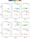 |
Fig. 1. Dn4000 (top) and Hβ (bottom) trends with age and metallicity. The indices are shown for a sample of 75 GCs for which a literature value of age is available, divided into six [Fe/H] bins and colour-coded according to it. In the background, the stellar models from BC16 relative to each [Fe/H] bin are shown with different line styles. |
Analogous to the Dn4000, in Fig. 1b the trends in age are shown for the Balmer index, Hβ, in comparison with the theoretical trends in the same metallicity bins. The distribution of this feature shows a good agreement with the models as well, this time decreasing with increasing metallicity.
Testing these observables against the stellar models in the case of GCs, objects for which independent and robust measurements of age and metallicities are available, is of great importance in order to validate the models and their use in cosmological analyses. In the application of cosmic chronometers (Jimenez & Loeb 2002), for instance, especially when the D4000 is directly used to trace the age evolution in redshift (Moresco et al. 2012; Moresco 2015; Moresco et al. 2016) it is fundamental that the D4000 traces correctly the stellar population evolution in time (i.e. the D4000–age slope).
3.2. Index–index diagrams
While in the previous section we studied the sensitivity of single features to the age and metallicity of the population, it is also possible to combine them in the analysis, taking advantage of their different sensitivity to parameters like age, metallicity, and alpha-enhancement. In this case, we are considering a different set of theoretical models to compare them with, specifically developed to take into account also a variation in the chemical composition (Thomas et al. 2011, TMJ). Historically, this method has been applied in galaxies (e.g. Onodera et al. 2015; Scott et al. 2017; Lonoce et al. 2020; Borghi et al. 2022) but also in GCs (e.g. Strader & Brodie 2004; Proctor et al. 2004; Mendel et al. 2007; Annibali et al. 2018) to derive constraints on the physical properties of these objects. Applying this method, we selected and compared indices that are mostly sensible to age, metallicity, or α-enhancement variations so that we could disentangle their contributions to the feature’s equivalent width. The most widely used are indices of the Balmer series, the iron-group ones, like Fe5270 and Fe5335, and Mgb. As for BC16, the models in TMJ have MILES resolution, but differently from BC16, they produce a forecast only for the set of Lick indices and not the entire spectrum. In particular, they model the indices values on a grid of ages, metallicities, and alpha-enhancements. Generally, an age-sensitive and a metallicity-sensitive index are plotted one against the other, and compared to a model grid with varying age and [Fe/H] but fixed [α/Fe]. In Fig. 2 we present two examples of these diagrams, Hβ − Mgb and HγF–[MgFe]’, where the latter is defined as:
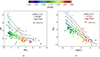 |
Fig. 2. Index–index diagnostic diagrams, on the left Hβ − Mgb and on the right HγF–[MgFe]’. The points are colour-coded by their literature value of [Fe/H]. We report TMJ models as a grid with varying metallicity (vertical lines) and varying age (horizontal lines), the first with the same colour code as the data points. Solid lines refer to models with [α/Fe] = 0.3, while the dashed lines in the background represent the solar-scaled grid. |
![Mathematical equation: $$ \begin{aligned} \mathrm{[Mg/Fe]^{\prime }} = \sqrt{\mathrm{Mg_b (0.72 \times Fe5270 + 0.28 \times Fe5335)}}. \end{aligned} $$](/articles/aa/full_html/2025/04/aa52812-24/aa52812-24-eq3.gif) (2)
(2)
Here, the [α/Fe] is fixed at 0.3, which is the closest to the typical value found in the literature for our sample of GCs, around 0.35 (e.g. Pritzl et al. 2005; Mendel et al. 2007).
This method allows us to obtain a first estimate of the population’s age and metallicity, which aligns well with the literature values, obtained with the independent traditional methods. In terms of age, the sample of GCs populates the area of the oldest objects in the diagrams, with a percentage of data points compatible with an age older than 12 Gyr of 66% and 88%, respectively, in the Hβ − Mgb and HγF–[MgFe]’.
From inspecting Fig. 2, we note that metal-rich GCs consistently fall below the oldest ages predicted by the models. To some extent, this may be caused by the lower α-enhancement characterising metal-rich GCs; the effect is indeed mitigated if we consider the dashed grey grid lines corresponding to models with [α/Fe] = 0. The observation that other metal-rich GCs exhibit similarly low Balmer line strengths compared to model predictions suggests a systematic problem with the zero-point calibration of current stellar population models2 (see Gibson et al. 1999; Vazdekis et al. 2015). Previous studies have shown that factors such as α-element enhancement and atomic diffusion (Cassisi et al. 1998; Salaris et al. 2000) in evolutionary models may provide a plausible explanation for the observed weakening of Balmer lines. These effects influence the temperatures of turnoff stars, which are the primary contributors to the Balmer lines in old, metal-rich stellar populations.
From the diagrams in Fig. 2 we can also see a small percentage of GCs in the area of typically younger objects, above the 8 Gyr grid-line. In particular, in the Hβ − Mgb this happens for 17 GCs, while in the HγF–[MgFe]’ for 11 GCs.
This behaviour can be attributed to the possible presence of an extended horizontal branch (HB), which can make the spectrum appear much bluer than expected for an old population and exhibit prominent Balmer lines, resembling a younger object. This is a very well-known effect, that has always made the study of GCs from integrated light challenging, mostly because the parameters determining the presence and the extent of the HB are not fully predictable with the current stellar evolution models. Various works have made progress in developing diagnostics to identify elongated HBs from integrated light, based on the Balmer lines (Lee et al. 2000; Schiavon et al. 2004) or on CaII and Mgb (Percival & Salaris 2011). Others have managed to include the HB contribution on top of the SSP models (Jimenez et al. 2004; Koleva et al. 2008; Cabrera-Ziri & Conroy 2022), modelling the emission from the HB hot stars as identified in the GCs’ CMD. However, we still lack of a complete modelisation of the HB component, due to the many uncertainties around its origin. Modelling the HB component is beyond the scope of this study, instead, our primary goal is to assess how this un-modelled component may impact studies of integrated populations, using methods commonly employed in galaxy evolution analyses.
The most common parameter used to quantify the HB extent is the morphology index HBR (Lee 1989; Lee et al. 1994), defined as:
 (3)
(3)
where B and R are the number of stars bluer and redder than the RR Lyrae instability strip, and V is the number of RR Lyrae stars. Although this parameter does not fully capture the distribution of stars along the HB, it still provides valuable information about the HB morphology, indicating whether it is predominantly red (HBR ∼ −1) or blue (HBR ∼ 1). In Fig. 3 we report the same Hβ − Mgb diagram as in Fig. 2a, but this time colour-coded by the HBR value listed in Harris (1996) (2010 edition), which is known for 69/82 objects (coloured points). According to this index, among the 14 GCs populating the area above the 8 Gyr grid line and for which the HBR is known, 13 show a blue HB, and for 11 of those the HBR is even higher than 0.5, a clue of a very elongated blue HB. The fraction of objects with HBR above zero decreases as we move to the areas belonging to older ages: 72% (18/25) between 8 Gyr and 12 Gyr and 33% (10/30) over 12 Gyr. The same trend can be observed moving from lower to higher [Fe/H], with a percentage of GCs showing blue HBs decreasing from 68% (23/34) at [Fe/H] < −1.35 to 49% (13/29) in the range −1.35 ≤ [Fe/H] ≤ −0.33 and dropping to zero at [Fe/H]> − 0.33.
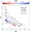 |
Fig. 3. Hβ − Mgb diagram, colour-coded by the value of HBR index. Blank points are GCs for which the HBR estimate is not available in Harris (1996) (2010 version). TMJ models are represented as a grid with varying metallicity (vertical lines) and varying age (horizontal lines). |
As was anticipated, stellar evolution models do not currently account for the presence of an extended blue HB, so this must be considered in the FSF analysis, where objects with extended HB morphology might be mistakenly identified as young stellar populations (Schiavon et al. 2004; Jimenez et al. 2004; Koleva et al. 2008; Cabrera-Ziri & Conroy 2022). From our initial qualitative analysis using indices, we expect this issue to be more prevalent in metal-poor objects with prominent Hβ, which tend to show the highest HBR.
4. Method and analysis
In this section, we present the method adopted to estimate the ages and physical properties of the GCs sample, the code used, its settings, and the results obtained.
4.1. Full spectral fitting with BAGPIPES
We performed FSF using the public code BAGPIPES (Carnall et al. 2018), which allows us to fit spectra and/or photometry adopting a parametric Bayesian approach. A detailed description of all the code’s features is presented in Carnall et al. (2019) and Carnall et al. (2022), while an overview of the settings that we adopt is already outlined in Tomasetti et al. (2023). Here, we recap the main features of the code, highlighting the aspects that are relevant to this work.
BAGPIPES is able to model synthetic spectra and photometry, based on a set of instructions, and then fit the so-modelled spectro-photometry to the observed one via a Bayesian approach, thus maximising the posterior probability using a nested sampling algorithm, Multinest (Buchner 2016). In this work, we focus on four main model components to construct the synthetic spectra.
The first component is an SSP model, which is designed to reproduce the continuum emission and the absorption features of a population built up in a single episode of star formation. The SSP models implemented in BAGPIPES are the 2016 version of Bruzual & Charlot (2003) (BC16, see Chevallard & Charlot 2016). They produce different synthetic spectra based on the wavelength λ range, the age of the stellar population, and its overall metallicity [Z/H], assuming a Kroupa (2001) initial mass function (IMF).
The second component is the star formation history (SFH). The code allows one to combine different SFHs, one for each SSP, but dealing with GCs we implement a single SFH, assuming a unique star formation episode. In particular, we adopt the delayed exponentially declining (DED) SFH, which is given by the equation
 (4)
(4)
where SFR is the star formation rate, τ provides the width of the SFH, and T0 sets the age of the Universe at which the star formation begins. Using a single DED is recommended when dealing with a stellar population whose timescale of formation is much shorter than its age, as we expect for GCs.
The third component is dust absorption and emission. This is particularly important to model the redder part of the spectrum, which can be largely depressed due to the presence of dust in the system. In the context of MW GCs, this component is necessary to account for the MW dust on the line of sight, for which WAGGS spectra are not corrected. The model implemented here is the Salim et al. (2018), represented by a power-law, as in Calzetti et al. (2000), with an additional parameter, δ, representing a slope deviation.
The last component is a non-physical term representing noise, which can be added to the error spectrum to account for any potential underestimation. This noise is introduced as white noise.
After running the code, we obtain a best-fit spectrum and the posterior distributions for all the parameters involved, like age, mass formed, overall metallicity, and dust extinction. At the same time, BAGPIPES can provide estimates of derived quantities, like the SFR or the stellar mass formed, parameters that are not directly involved in the fit. In particular, the mass formed (Mformed) and the stellar mass formed (M⋆) are different in that the first one comprises all the mass formed from t = 0 to the time t at which the GC is observed:
 (5)
(5)
including also stellar remnants (Mrem), while the second one includes only the mass of living stars:
 (6)
(6)
From now on, we refer to M⋆ as the mass of the objects.
Since we aim to use the resulting ages in a cosmological framework, it is important to avoid any constraint based on cosmology. For this reason, we employ a version of BAGPIPES, described in Jiao et al. (2023), that deviates from the original in handling the priors on the stellar population age, allowing them to vary up to a cosmology-independent value (e.g. 15 Gyr, 20 Gyr) at any redshift. This modification has already been tested and validated in VANDELS (Tomasetti et al. 2023) and LEGA-C (Jiao et al. 2023). Originally the code assumes a cosmological prior on ages, for which the maximum age resulting from the fit should be smaller than the age of the Universe at the corresponding redshift, given a flat ΛCDM model with parameters ΩM = 0.3, ΩΛ = 0.7 and H0 = 70 km s−1 Mpc−1. Although this effect is of relative interest in stellar population studies and is typically neglected, it can’t be ignored in cosmological analyses because the derived ages would be constrained by the cosmological model assumed, leading to results that just recover the assumed prior. Below, we are going to test the effect of different assumptions of age prior on the sample of GCs.
4.2. Full spectral fitting in WAGGS
Before inputting the cluster spectra into BAGPIPES, some adjustments were necessary. First, we downgraded the spectral resolution to approximately 2.7 Å FWHM, consistent with the BC16 models used in the code. Next, we aligned the spectra to the correct frame using distances from Baumgardt et al. (2023) and corrected for radial velocity variations, which could cause minor blueshifts or redshifts in the spectra. To prevent underweighting the blue features in the fit – due to the non-uniform error spectrum, with S/N ranging from a few tens to a thousand – we set an upper limit for the S/N at 100 and adjusted the error spectrum accordingly. We tested various S/N thresholds (e.g. 20, 50), finding that they had minimal impact on the results, except when the S/N ratio between the blue and red ends of the spectrum differed by more than a factor of ten, which resulted in very low weight for the blue features in the fit.
After these adjustments, we performed multiple tests to optimally use BAGPIPES on GCs spectra and find the best-fit configuration to reproduce their spectral features accurately. In particular, this process involved: adopting different SFHs (e.g. single burst, delayed exponentially declined) with different priors on the parameters; fitting different wavelength ranges, either moving the lower limit to longer wavelengths to reduce the contamination by HB stars or pushing the upper limit to redder features to better constrain dust reddening; testing different priors on the GC’s [Z/H] and mass (e.g. uniform, Gaussian, logarithmic) to assess their impact on the estimation of these parameters, as well as the influence on ages, given the degeneracies at play. It is worth mentioning here that the mass and metallicity estimates proved to be very stable against all the different changes in the fit setup, while ages were mainly affected by the choice of prior, as we discuss in the following.
In the end, we converged to a fit configuration in which: (i) as often done in literature (Koleva et al. 2008; Gonçalves et al. 2020) we fit the range 3700–6000 Å to avoid the redder telluric lines and we mask the interval 5870 − 5910 Å, where the spectra show a very deep sodium doublet absorption line, since it could be potentially contaminated by interstellar absorption; (ii) we consider a single DED SFH, a dust component and a noise component; (iii) on all the parameters we set uniform, uninformative priors.
To assess the impact of the cosmological prior on the results, we tested two different upper limits for the age parameter: 13.47 Gyr, age of the Universe in a flat ΛCDM model with ΩM, 0 = 0.3, ΩΛ, 0 = 0.7, H0 = 70 km/s/Mpc; 15 Gyr, a loose limit independent of any cosmology. We refer to the first configuration as Config. 13.5 and to the latter as Config. 15. A summary of the main parameters and relative priors for the two configurations can be found in Tab. 1. We highlight that we assume uniform priors on all the parameters, along with wide ranges so that the results are not constrained by any previous knowledge of the GC’s mass, metallicity, dust extinction or age.
Parameters and priors for different configurations.
As was anticipated, BAGPIPES adopts the overall metallicity [Z/H] as the metallicity parameter. To compare our results with [Fe/H] values from the literature, we need to perform a conversion. We used the conversion formula from Salaris & Cassisi (2005):
![Mathematical equation: $$ \begin{aligned} \mathrm{[Z/H]}&= \log \left(\frac{Z}{Z_\odot }\right) \nonumber \\&= \mathrm{[Fe/H]} + \log _{10}\left(10^{[\alpha /\mathrm{Fe}]} 0.694 + 0.306\right). \end{aligned} $$](/articles/aa/full_html/2025/04/aa52812-24/aa52812-24-eq8.gif) (7)
(7)
For objects with [Fe/H]≤ − 1, we applied this formula with an alpha-enhancement of [α/Fe] = 0.35, which is typical of the metal-poor MW GCs (e.g. Pritzl et al. 2005; Mendel et al. 2007), while for GCs with [Fe/H]> − 1 we use [α/Fe] = 0.15, average alpha-enhancement at these metallicities (see, e.g., Pagel & Tautvaisiene 1995; Pancino et al. 2017). From now on, we refer to the quantity [Z/H] as the metallicity of the GCs.
It should be noted that in this work, due to their integration within the BAGPIPES framework, we adopted the BC16 models, which rely on solar-scaled evolutionary tracks. We recognise that this approach can lead to slightly older age estimates compared to α-enhanced isochrones of similar metallicity (Salasnich et al. 2000; Thomas & Maraston 2003). Alternative SSP models that include non-solar compositions and adequate metallicity coverage (Thomas et al. 2003, 2004; Lee & Worthey 2005) typically have a maximum age of 12–15 Gyr (see, e.g., Proctor et al. 2004; Mendel et al. 2007, for discussion). Consequently, they do not enable the removal of the age prior as effectively as required for this analysis. We emphasise the need for models with non-solar compositions to refine age estimates in future studies.
4.3. Results
We performed a visual inspection to evaluate the quality and convergence of the fits. Specifically, we identified fits that either failed to recover the spectral lines or continuum or exhibited double- or multiple-peaked posterior distributions. As a result, we discarded a significant number of poor fits, totalling 11 objects in both Config. 13.5 and Config. 15, which represent about 14% of the sample. Among these, eight GCs had an HBR > 0, and we found that, in these cases, the posterior spectrum underestimated the emission in the wavelength range bluewards of 4000 − 4500 Å. This issue is likely due to the blue HB emission, which the models cannot fully reproduce. Consequently, the fits converge to younger ages, as is observed in these cases in which all eight poor fits have ages younger than 10 Gyr. As is discussed in Sect. 3.2, various studies have successfully included a contribution of the HB on top of the SSP models (e.g. Jimenez et al. 2004; Koleva et al. 2008; Cabrera-Ziri & Conroy 2022). However, incorporating this component into BAGPIPES is outside the scope of this work. Removing bad fits, the clean sample counts 66 GCs in both configurations.
In Fig. 4 two examples of good fits are reported, both converging to ages older than 13 Gyr, one presenting a red HB (NGC6356, HBR = −1) while the other shows a blue HB (NGC 6717, HBR = 0.98). The pulls highlight how in the case of NGC6356 the stellar models, plus the dust components, are able to accurately reproduce the GC’s spectrum, with residuals compatible with 1-σ fluctuations at all wavelengths. In the case of NGC6717, the quality of the fit is still good, but the pulls clearly show a residual at bluer wavelengths, especially concerning the Balmer absorption lines, pointing out the unmodelled hot stars component. This suggests that for GCs characterised by blue HBs may still produce a reliable age estimation, as long as the blue HB stars do not outshine the blue end of the spectrum.
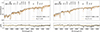 |
Fig. 4. Examples of good fits. In the top panels, the observed spectra are shown in black and the posterior ones in orange. Dashed lines identify the Balmer absorption series, while other main absorption features are highlighted with shaded grey boxes. In the bottom panels, the pulls of each fit ((observed – fit)/error) are shown, with the orange horizontal area representing a 1-σ fluctuation. |
The quality of both considered setups is highlighted by the median reduced chi-squares,  in Config. 13.5 and
  in Config. 15. This is quite noticeable since in this case we adopted the formal spectrum error provided by the analysis, with the correction described in Sect. 4.2. These values are further (as was expected) reduced if we take into account the noise parameter, which acts in correcting the error spectrum for potential underestimations, leading to
  in Config. 13.5 and
  in Config. 15. To analyse the derived physical properties, we consider, for each parameter, the median and the 16th and 84th percentiles of the posterior distribution, respectively, as the best-fit value, lower and upper error.
4.3.1. Configuration 13.5
In Config. 13.5 we observe that metallicities and GC masses are in good agreement with literature values, with mean deviations of ⟨Δ[Z/H]⟩ = 0.09 ± 0.21 dex and ⟨Δlog(M⋆/M⊙)⟩ = −0.09 ± 0.24 dex, respectively, consistent with the typical errors associated with these quantities (see Sect. 2). In terms of stellar age, instead, a clear bimodality is present. While 17% of the sample (11 GCs) turns out to have ages older than 10 Gyr and only ∼0.16 Gyr younger than literature values on average, most of it (55 GCs) shows ages significantly younger than 10 Gyr, ∼8.9 Gyr lower on average. We investigate this difference in the following.
In Figs. 5a and b we show the differences in stellar mass and metallicity as a function of this age gap, colour-coded by HBR index. This highlights two important aspects.
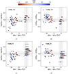 |
Fig. 5. Differences in stellar mass (Δlog(M⋆/M⊙)) and metallicity (Δ[Z/H]) as a function of the difference in age as estimated in this work with respect to literature values. The dashed lines correspond to a null difference, and the shaded grey areas represent an average representative error on literature values, namely 0.2 dex in mass, 0.15 dex in metallicity and 1.5 Gyr in age. The top two panels refer to Config. 13.5 while the bottom ones to Config. 15. All the points are colour-coded by their HBR index. |
The first is, again, the trend with HBR, showing that when this index is positive (blue HB), the code misinterprets the blue shape of the spectrum and the deep Balmer lines for a young population 87% of the time (27/31), resulting in ages on average 8.4 Gyr younger than expected from the literature. This exact behaviour is also observed for most of the red HB population, but in a smaller fraction (73% of the cases, 19/26 GCs) and with a less significant age discrepancy of 5.1 Gyr on average. A similar result was already found both in Koleva et al. (2008) and Cabrera-Ziri & Conroy (2022), where the issue was mitigated by adding a fraction of hot stars on top of the SPS models, but, as was anticipated, including the HB component goes beyond the purpose of this work. In Sect. 4.6, though, a detailed comparison with the results in Cabrera-Ziri & Conroy (2022) can be found.
The second is the existence of a degeneracy among the parameters involved. A lower cluster mass or a higher metallicity can easily mislead the fit to ages much younger than the literature one. This is clear if we compute the median differences in metallicity and mass separately for the GCs resulting older and younger than 10 Gyr: for the former, we find average deviations of ⟨Δ[Z/H]⟩ = −0.14 ± 0.19 dex and ⟨Δlog(M⋆/M⊙)⟩ = 0.16 ± 0.15 dex, for the latter instead ⟨Δ[Z/H]⟩ = 0.13 ± 0.18 dex and ⟨Δlog(M⋆/M⊙)⟩ = −0.13 ± 0.24 dex.
4.3.2. Configuration 15
In Config. 15 the good agreement of metallicity and GC mass estimates with literature values holds, with average differences of ⟨Δ[Z/H]⟩ = −0.02 ± 0.23 dex and ⟨Δlog(M⋆/M⊙)⟩ = 0.04 ± 0.28. Concerning the stellar ages, even though the only difference with respect to Config. 13.5 is the removal of the cosmological prior, the results improve significantly. Here 36% (24 GCs) of the sample shows ages older than 10 Gyr, more than twice the old population of Config. 13.5. Among these 24 GCs, the ages result compatible with literature values 92% of the times (22 GCs), on average 0.67 Gyr older, and we find average discrepancies in [Z/H] and mass of Δ[Z/H]= − 0.11 ± 0.18 and Δlog(M⋆/M⊙) = 0.20 ± 0.20.
In Figs. 5c and d we show the analogous of Figs. 5a and b for Config. 15. We can see that both the trend in HBR and the age–metallicity and age–mass degeneracies are present but with important differences. This time, removing the upper limit on the age parameter has reduced the fraction of blue HB GCs mistaken for young populations to 71% (22/31) and the one of the red HB GCs to 54% (14/26). This means that 13 GCs previously resulting younger than 10 Gyr are now recognised as old populations, representing a 20% increment. The degeneracies cited above play an important role in this because all of these 13 GCs are here characterised by a lower metallicity (Δ[Z/H]∼ − 0.18 dex) and a higher mass (Δlog(M⋆/M⊙)∼0.19 dex) than the one found in Config. 13.5, yet mostly in agreement with literature values within errors. This suggests that for a fraction of GCs an old, more realistic solution does exist beyond the cosmological limit usually set when performing FSF and that it may also be preferred to the younger one if this area of the parameter space is made accessible. For this reason and in light of the subsequent cosmological analysis, we consider Config. 15 our benchmark.
4.4. Systematic effects
As was anticipated in Sect. 4.2, we performed multiple tests with different settings to find the optimal fit configuration. These analyses have been used to assess the systematic error induced in the age determination with our approach. Specifically, we examined eight configurations, each differing from our benchmark in one or two key aspects, including variations in SFH type (burst or DED), age prior (15 Gyr or 20 Gyr) metallicity prior (uniform or Gaussian), wavelength range of the fit, and in fitting spectra in physical units or normalised in the window 4500–5000 Å. The latter was applied in just one configuration, the only case in which the mass parameter could not be determined due to the normalisation. All the characteristics of the different configurations are outlined in Tab. 1, numbered from one to eight.
In this analysis, we discarded all the spurious young solutions with a best-fit age below 10 Gyr for the same reasons discussed in Sect. 4.3, and all the bad fits in Config. 15 and in each of the eight test configurations. In this way, we end up with a sample of 18 GCs having a good fit in at least five out of the nine runs. For each object, we computed the standard deviation of the age distribution in the nine runs. Finally, we estimated a global systematic contribution to the age uncertainty as the average of these standard deviations, weighted on the number of good fits for each GC, resulting in 0.71 Gyr3.
In addition, we considered the possibility of a systematic effect induced by mass segregation. The large apparent sizes of Galactic GCs on the sky, combined with the relatively small field of view of the WiFeS spectrograph (38 × 25 arcsec, comparable to the median core radius of an MW GC, Harris 2010), pose significant challenges for integrated light observations of Galactic GCs. Usher et al. (2017) used a single, central pointing for each GC in their study. However, the MW GCs in their sample span a wide range of heliocentric distances – from 2.2 kpc for NGC 6121 to 41.2 kpc for NGC 7006 – causing the fraction of GC light sampled to vary considerably. When the WiFeS field of view covers only a small portion of a GC’s area, stochastic effects may prevent proper sampling of all stages of stellar evolution, particularly in lower-mass clusters. Additionally, mass segregation – whereby more massive stars migrate towards the cluster centre due to dynamical evolution – further complicates observations. This effect alters the slope of the mass function with radius (e.g. Beccari et al. 2015), potentially mimicking weak radial variations in the IMF. To assess these biases, we examined potential correlations between the age differences estimated in this work and those reported in the literature, as well as with cluster mass and the ratio of the core radius or half-light radius to the equivalent radius of the WiFeS field of view (17.4 arcsec). We found no evidence of statistically significant correlations among these quantities.
4.5. The role of metallicity
In Sect. 3.2 we observed that not only the presence of an extended blue HB, but also a low metallicity could produce some spectral features that can drag the fit to younger ages due to their degeneracy. Here we want to verify if this trend is present in our results. In Fig. 6a, we plot the metallicity obtained from our fit against the values found in the literature, colour-coded by the difference between the age estimated from the fit and the literature one. We can observe that the best match in age estimation is indeed found at the highest metallicities, while the objects for which the age is most underestimated are also the ones with lower metallicity. To perform a quantitative comparison, we divided our sample into metallicity sub-samples, considering three intervals equally spaced in [Z/H]lit: a metal-rich [ − 0.7, 0.0], a metal-intermediate [ − 1.4, −0.7] and a metal-poor [ − 2.1, −1.4].
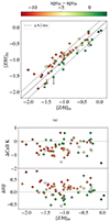 |
Fig. 6. Metallicity and differences in CaII K and Hβ measurements as a function of literature metallicity. Top: [Z/H] obtained in this work against literature [Z/H], colour-coded by the corresponding difference in age. The continuous line represents the one-to-one relation, and the dashed lines the 0.2 dex scatter. Bottom: differences in CaII K and Hβ as measured on the posterior spectra with the observed ones, colour-coded by the difference in age. |
The metal-poor sample counts 15 GCs, among which only the 20% (3/15) is recognised as older than 10 Gyr. This can be better understood by examining the top panel of Fig. 7, where the median stacked spectrum of the metal-poor sample is compared to two synthetic spectra, one 13 Gyr old and the other 4 Gyr old, while all the other parameters (e.g. [Z/H], mass, dust) are fixed to the median literature values characterising this sub-sample. The spectral shape does indeed resemble the one of a young population, with a stronger emission bluer than ∼ 4400 Å with respect to the spectrum of an old population, and stronger Balmer lines. However, in Fig. 6b, where discrepancies in the reproduction of CaII K and Hβ are shown as a function of literature metallicity, we can see that for most of the metal-poor GCs, the Hβ line is actually overestimated. This means that the young solution, even if preferred by the fit, does not precisely follow the observed features. In terms of metallicity and mass, the agreement with literature values is very good, with average deviations of ⟨Δ[Z/H]⟩ = −0.02 ± 0.35 dex and ⟨Δlog(M⋆/M⊙)⟩ = −0.2 ± 0.2 dex, respectively.
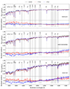 |
Fig. 7. Stacked spectra of the metal-poor (top panel, [ − 2.2, −1.4]), metal-intermediate (central panel, [ − 1.4, −0.6]) and metal-rich (bottom panel, [ − 0.6, 0.2]) subsamples, in comparison with a 4 Gyr (in blue) and 13 Gyr old (in red) synthetic spectra. The values of mass, dust absorption and velocity dispersion of the synthetic spectra are set to the median literature values of each subgroup. All the spectra are normalised in the window 4500–5000 Å. At the bottom of each panel the residuals of the stacked spectra with respect to the synthetic ones are shown with corresponding colours. The Balmer series is indicated with dashed lines, other relevant spectral features are highlighted with grey boxes. It can be noticed how the different sub-groups show different continuum and spectral features properties, and how the models are able to reproduce more accurately the high-metallicity ones. |
The metal-intermediate is the largest sub-group, with 33 GCs, and shows a higher percentage of GCs older than 10 Gyr compared to the metal-poor sample, equal to 33% (11/33). Its median stacked spectrum has a better agreement with an old population in terms of the continuum but still fails to reproduce some observed lines of the Balmer series, as we can see in the central panel of Fig. 7. This is mostly evident for the Hβ line, falling in the region 4500−5000 Å where the spectra have been normalised, which is clearly better reproduced by a young population, as in the metal-poor case. This suggests that there is still non-negligible contamination by hot stars, deepening the Balmer series. We can observe this in more detail in Fig. 6b where to obtain old solutions, the fit has to underestimate the Hβ feature. In contrast, for the young ones, it is either compatible with observations or overestimated. In this metal-intermediate group, we can also observe the importance of reproducing the CaII K line in recovering ages. In fact, while the old solutions all scatter around ΔCaII K ∼ 0, the young ones systematically underestimate this feature. Regarding the metallicity, this sub-group shows a good agreement with literature values, with a ⟨Δ[Z/H]⟩ = 0.10 ± 0.15 dex, and a discrepancy in mass smaller than before ⟨Δlog(M⋆/M⊙)⟩ = −0.04 ± 0.30 dex.
In the metal-rich sample instead, we are able to obtain ages older than 10 Gyr for 56% (10/18) of the sample. This fraction increases as we move to solar values, reaching 70% for [Z/H]lit ≥ −0.4. In the bottom panel of Fig. 7 we can see that, among the three samples, the metal-rich is the most distant from a young population with a much redder continuum. In addition, the metal-rich is the only stacked spectrum in which the Hβ region is better reproduced by the old synthetic spectrum instead of the young one, even if a residual, going in the opposite direction, is still visible4. Looking at Fig. 6b, the metal-rich sample is the only one for which both Hβ and CaII K are well reproduced. In terms of metallicity and mass here we find ⟨Δ[Z/H]⟩ = −0.08 ± 0.15 dex and ⟨Δlog(M⋆/M⊙)⟩ = 0.09 ± 0.16 dex with respect to literature values.
The fact that we can recover ages well in this metallicity range is a remarkable result also in the context of galaxy evolution studies, for which GCs have always been an important test bench, since it shows the reliability of the FSF method in recovering the main physical parameters of the stellar population in a metallicity interval that is typical of high redshift galaxies (see, e.g., Kriek et al. 2019; Lonoce et al. 2020; Carnall et al. 2022; Borghi et al. 2022). Moreover, we show that spectral features like Hβ and CaII K prove to be very sensible to possible spurious age determinations and thus can be used as diagnostics to determine the quality of the age estimates.
4.6. Comparison with previous works
As was anticipated in Sect. 1, different works have already been published investigating the potential of analysing GCs’ integrated spectra, either relying on different datasets or adopting different fitting codes. Here we focus on the work from Cabrera-Ziri & Conroy (2022) (CC22, hereafter), where they use the observations from Schiavon et al. (2005) for a common sub-sample of GCs, and then on the results from Gonçalves et al. (2020) (G20, hereafter), where they analyse the same data but adopt a non-parametric approach.
4.6.1. Comparison with Cabrera-Ziri & Conroy (2022)
CC22 used a similar, but non-parametric, FSF approach with the code ALF (Conroy & van Dokkum 2012) to estimate the ages and metallicities of 32 Galactic GCs from Schiavon et al. (2005), fitting normalised spectra in the range ∼3300 − 6500 Å. As in Config. 13.5, CC22 initially performed the analysis with a standard setting, using a cosmological prior of 14 Gyr. They obtained ages compatible with literature values within 1.5 Gyr for seven GCs, which constitutes 22% of their sample. To compare the results, we consider the 31 GCs included both in their sample and our good fits. For those, in Config. 13.5 we obtain ages within 1.5 Gyr from literature values for 13% of the sample (4/31) while this fraction is more than doubled when we remove the cosmological prior, reaching 32% (10/31).
Compared to CC22, the performance in recovering old ages with Config. 13.5 is comparable but slightly worse. This is likely due to the additional degrees of freedom in our setting, such as the inclusion of dust and mass parameters, along with the lower age prior. If adopting a multi-component model can help in reproducing all the spectral features in more detail, this approach is also more prone to possible degeneracies, as we underlined in different steps of our analysis. Nevertheless, this same choice allows us to obtain better results when removing the cosmological prior, with an increase in the fraction of old objects of 20% with respect to our Config. 13.5 and 10% with respect to the standard setting in CC22.
In CC22, an additional fit was performed that included a component to account for the hotter fraction of HB stars. This approach allowed them to recover ages older than 10 Gyr for 27 out of 31 GCs, with 24 of these being compatible with literature values within 1.5 Gyr. As already discussed, modelling the HB component is outside the purpose of this work, but represents a promising possibility to be explored in future analyses.
4.6.2. Comparison with Goncalves et al. (2020)
In G20 the authors focus on the impact that the wavelength range choice has on the results, adopting the FSF code STARLIGHT (Cid Fernandes et al. 2005). They fit normalised spectra using MILES SSP models (Vazdekis et al. 2015) with ages up to 14 Gyr, [Fe/H] in the range from −2.27 to 0.26 and alpha enhancement either absent or equal to 0.4. Dust reddening is implemented in the code, modelled as in Cardelli et al. (1989). We compare our results to the ones published in Goncalves et al. (2023), obtained by fitting the interval 4828–5634 Å, a narrow range where the main features detectable are Hβ, Mgb triplet, Fe5015, Fe5270, and Fe5335.
We consider the 58 MW GCs for which we obtain a good fit among the 64 MW GCs published in G20; in this sample, they obtained ages compatible with literature values within 1.5 Gyr for nine GCs, representing 15% of the total. In this same sub-group, we have seven GCs compatible with literature ages in Config. 13.5, and 15 in Config. 15, corresponding to 12% and 26% of the sample, respectively. As in the comparison with C22, also in the case of G20 our results when the cosmological prior is applied are comparable but slightly worse, and as commented above the reason probably resides in the higher number of parameters involved and the lower age prior. Again, when we remove the cosmological prior, we obtain a major improvement in the fraction of ages compatible with literature, both with respect to our Config. 13.5 (+14%) and to G20 (+11%).
It is worth mentioning here that we also tested the impact on the results of fitting the wavelength range adopted in G20, first suggested in Walcher et al. (2009), and we considered it when computing the systematic uncertainty on ages in Sect. 4.4. Avoiding all the features bluer than 4828 Å, polluted by the hot HB component, this configuration performs much better for the blue HB, low-metallicity GCs in our sample. In particular, it allows us to recover ages older than 10 Gyr for 63% of metal-poor GCs and 73% of metal-intermediate ones. For the metal-rich sample, instead, it yields worse results compared to Config. 15, with 47% of GCs resulting older than 10 Gyr. Nevertheless, the latter sub-group is the one in which the stellar models should be most effective, thanks to the absence of an extended HB component and low alpha-enhancement in the systems, so Config. 15 was still preferable in terms of the robustness of the results.
5. Application to cosmology
In this section, we analyse what impact our results for GCs’ ages, interpreted as lower limits on the age of the Universe, tU, can have in the determination of the Hubble constant H0 (Jimenez et al. 2019; Valcin et al. 2020, 2021; Vagnozzi et al. 2022; Cimatti & Moresco 2023).
5.1. Method
As anticipated in Sect. 1, and widely described in Cimatti & Moresco (2023), H0 is very sensitive to the value of tU. In a generic cosmological model, H0 can be expressed as:
 (8)
(8)
where t is the age of a given object, zF its redshift of formation, E(z) is defined as H(z)/H0 and A = 977.8 converts the result in units of km s−1 Mpc−1. The analytical expression of E(z) depends on the cosmological model assumed, in particular, in a flat ΛCDM model it can be expressed as a function of redshift and matter density parameter ΩM, so that H0 becomes:
![Mathematical equation: $$ \begin{aligned} {H_0 = \frac{A}{t}\int _0^{z_F}\frac{1}{1+z}[\Omega _{\rm M}(1+z)^3+(1-\Omega _{\rm M})]^{-1/2} \mathrm{d}z}. \end{aligned} $$](/articles/aa/full_html/2025/04/aa52812-24/aa52812-24-eq14.gif) (9)
(9)
Considering the limit of zF = ∞ for which t corresponds to the age of the Universe tU, we can easily understand the sensitivity of the method. Fixing ΩM = 0.3 and varying tU from 12.9 Gyr to 14.1 Gyr the resulting value of H0 spans from 73 km s−1 Mpc−1 to 67 km s−1 Mpc−1.
When applying the method to the oldest objects, H0 can be estimated via a Bayesian approach, in which the likelihood is built on the difference between the measured age and the one predicted by the cosmological model (agem), accounting for the age error (σage):
![Mathematical equation: $$ \begin{aligned} {\mathcal{L} (\mathrm{age}|\mathbf p ) = -0.5 \sum _i \frac{[\mathrm{age}_i-\mathrm{age}_m(\mathbf p )]^2}{\sigma _{\mathrm{age},i}}}, \end{aligned} $$](/articles/aa/full_html/2025/04/aa52812-24/aa52812-24-eq15.gif) (10)
(10)
where p = (H0, zF, ΩM) in a flat ΛCDM cosmology. The posterior distribution then, can be sampled with a Monte Carlo Markov chain approach like the one implemented in the affine-invariant ensemble sampler emcee (Foreman-Mackey et al. 2013). In the choice of priors, a flat, uninformative one can be adopted on H0 and zF, while a Gaussian prior is preferable for ΩM in order to break its intrinsic degeneracy with H0.
As a final note on the method, it is interesting to highlight that nowadays, with facilities like JWST, this approach is no more limited to the study of local objects but can be extended to higher redshift thanks to the first detections of GCs around lensed galaxies. A great case-study is the one of the Sparkler, a galaxy discovered in Webb’s First Deep Field (Mowla et al. 2022) showing a population of compact objects associated with it. Among the 18 compact objects identified (Mowla et al. 2022; Millon et al. 2024), Sparkler shows five GC candidates that, if confirmed with spectroscopy, would be the first detection of GCs at z = 1.38. The spectroscopic study of these objects, analogous to the one performed in this work, would allow us to measure their age, potentially with a higher precision than the one obtained here for ∼13 Gyr old GCs. In younger stellar populations, indeed, the shape of the spectrum and the width of the absorption lines changes much quicker than it does at very old ages, thus reducing the impact of the parameters’ degeneracies on the age uncertainty. In the context of our cosmological analysis, extending the method at higher redshift would just require to replace the lower limit of the integral in Eq. (9) with the redshift of the lensed GC. In the case of the Sparkler at redshift 1.38, for example, the age of the Universe ranges from 4.3 Gyr to 4.7 Gyr adopting the reference values for H0 given above, 73 km s−1 Mpc−1 and 67 km s−1 Mpc−1, respectively.
5.2. Results
As was anticipated in Sect. 4.3, we adopted as benchmark Config. 15, where the cosmological prior is removed. To identify the tail of the oldest objects, we adopt a Gaussian Mixture Model (GMM) on the whole sample, combining normal distributions peaked on the best-fit ages, with 1-σ equal to relative uncertainties. We then let the fit decide the optimal number of subsamples in which to split our data. Both considering the Bayesian Information Criterion (BIC) or the Akaike Information Criterion (AIC), we find that the optimal number of components is three: a first peak identifying the youngest, blue-HB, spurious solutions; a second one for the intermediate ages; a third one comprising all the 24 oldest GCs, peaking at 13.4 ± 1.1 Gyr. The latter represents the oldest tail of the GCs’ age distribution.
We applied the method described in Sect. 5.1 for each of these GCs separately, and then on their average, adopting the following priors: uniform on H0 ∈ [0, 150] km s−1 Mpc−1 and on zF ∈ [11, 30], Gaussian on ΩM = 0.30 ± 0.02. The lower limit on zF is based on the highest redshift at which galaxies have spectroscopic confirmations (Curtis-Lake et al. 2023), the higher limit instead relies on the values found in theoretical models for the redshift of formation of the very first stars (Galli & Palla 2013). As regards ΩM, the value chosen here comes from the combination of different low-redshift results (Jimenez et al. 2019), thus independent of the CMB.
Our 24 old GCs span the age range 13.2–13.6 Gyr, with errors around 1 Gyr, thus the resulting H0 range we find covers the interval 69.5–71.7 km s−1 Mpc−1, with typical uncertainties of ∼5 km s−1 Mpc−1. To provide a single H0 measurement, we also ran the MCMC using mean and standard deviation of the old peak found in the GMM fit: 13.4 ± 1.1 Gyr. This results in a final value for  (stat).
To account for the systematic contribution to the error budget computed in Sect. 4.4 we summed it in quadrature to the standard deviation of the distribution and ran again the MCMC. The final result, comprising both statistics and systematic effects is:

In Fig. 9 the 24 GCs’ ages and the corresponding H0 estimates found after the MCMC run are represented as Gaussian distributions, in the respective domains and combined as ellipses in the H0–age plane. The corresponding Gaussian curves and ellipses relative to the combined age and H0 are shown as solid black lines. For comparison, the values from Riess et al. (2022) and Planck Collaboration VI (2020) are represented, respectively, with dashed and dotted lines.
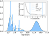 |
Fig. 8. Combination of all the 66 GCs ages, drawn as normal distributions peaked on the best-fit value and 1-σ equal to the associated error. In black, the three Gaussian components identified with a GMM are shown. In the inner panel, AIC and BIC curves are shown. |
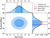 |
Fig. 9. H0 versus age for the sample of 24 old GCs. The ages and corresponding H0 estimates are shown as Gaussians peaked on the best-fit values and 1-σ equal to the relative uncertainties. The 1-σ limits are also highlighted in a darker blue. The solid black curves correspond to the average GC’s age and relative H0 estimate. For comparison, the values from Riess et al. (2022) and Planck Collaboration VI (2020) are represented, respectively, with dashed and dotted lines in the H0 domain, and in the age-domain we report the corresponding ages of the Universe as computed in a flat ΛCDM with ΩM = 0.3 and ΩΛ = 0.7. |
Of course, the results that we obtain here are not able to address the tension. Still, they represent a pilot exploration of the use of GCs’ ages for cosmological purposes, especially in view of future missions that could potentially discover such objects at higher redshifts.
6. Conclusions
In this work, we analysed the integrated spectra of a sample of 77 MW GCs from the WAGGS project (Usher et al. 2017) and measured their physical properties via FSF with the code BAGPIPES (Carnall et al. 2018). In doing this, we aimed to study how well FSF can recover the GCs’ ages and physical parameters, and assess, in particular, how the age estimates are affected by the presence or absence of a cosmological prior. This required a modification on the code, already tested and validated in Jiao et al. (2023) and Tomasetti et al. (2023), thanks to which a flat non-cosmological prior can be set at 15 Gyr. At the same time, this allowed us to obtain a cosmology-independent lower limit on the age of the Universe, that we used to derive a new constraint on H0, performing a pilot study for future potential applications at higher redshift.
Our results are summarised as follows:
-
Measuring age-related spectral features detectable in the spectra, like Dn4000 and Hβ, allowed us to build index-age diagrams for these features in different metallicity bins, showing a distribution that well aligns with the trends from theoretical spectral models.
-
Combining age-related and metallicity-related spectral features we built two different types of index–index diagrams, Hβ − Mgb and HγF–[MgFe]’, able to disentangle age and metallicity contributions to the spectral features. Based on how the GCs populated these diagrams, we could have a first estimate of their properties, showing an overall good agreement with the corresponding literature values. Ages, however, appeared underestimated for a fraction of the sample characterised by low metallicity ([Fe/H] < −0.33) and blue HB (HBR > 0), that, showing a more prominent Hβ, populated the area of ages younger than 8 Gyr. This anticipates how the presence of an unmodelled HB component in the spectra can bias the results towards younger solutions.
-
Performing FSF with BAGPIPES we could measure simultaneously the age, metallicity, and mass of the GCs. We tested multiple fit configurations, with different choices of priors, model components, SFHs, and wavelength ranges. Metallicity and mass proved to be very stable against the changes in fit configurations, while age was mostly sensible to the prior limit. In particular, we tested two configurations, one with a cosmological prior set at 13.5 Gyr and another at 15 Gyr (Config. 15), thus independent of cosmology. The percentage of GCs for which ages result compatible with the literature values within ±1.5 Gyr increases by 20% removing the cosmological prior, demonstrating the relevance of this limit in stellar population studies. In Config. 15 the agreement with literature values is maximum for the sub-group of GCs with [Z/H] > −0.4, the least affected by the presence of blue HBs, reaching 70%. Metallicity and mass always result well compatible with reference values independently of HBR, [Z/H] or fit setting, with average discrepancies on the whole sample of ⟨Δ[Z/H]⟩= − 0.02 ± 0.24 dex and ⟨Δlog(M⋆/M⊙)⟩ = 0.04 ± 0.28, compatible with the typical uncertainties associated with these quantities.
-
Performing a GMM fit on the whole age distribution as derived in Config. 15, we identified a tail of 24 old GCs with ⟨age⟩ = 13.4 ± 1.1 Gyr. In a cosmological framework, this value can be used as a lower limit on the age of the Universe to constrain the Hubble constant. In particular, by fitting the H0 − tU relation in a flat ΛCDM cosmology and assuming Ωm = 0.30 ± 0.02, from low-z measurements, we obtained
 . Taking into account a systematic contribution to the age error of 0.71 Gyr, based on the age fluctuations in eight different fit configurations, we obtained:
While we acknowledge that the method adopted in this paper is not intended to compete with other age estimation techniques (e.g. isochrone fitting) for local and resolved objects, it does offer a viable alternative. In addition, high-quality spectra comparable to WAGGS are unlikely to be obtained in the near future for cosmologically relevant GCs, particularly in terms of signal-to-noise ratio, resolution, and wavelength coverage. Therefore, it is crucial to extend these types of studies to spectra that are realistically obtainable in the near or intermediate term. In Tomasetti et al. (2024), for instance, we expand on the analysis presented here by applying it to the multiwavelength photometry of GCs observed in the Sparkler galaxy (Mowla et al. 2022), aiming to explore the potential for deriving reliable, cosmology-independent ages using photometric data alone.
Finally, it is worth noting that detailed modelling of HB populations – or other stellar populations such as blue stragglers – may not significantly affect studies of GCs at higher redshifts. A well-populated HB typically emerges only in clusters older than 6–8 Gyr. For the Sparkler GCs, with predicted ages of less than 4 Gyr at z = 1.38 (Mowla et al. 2022; Claeyssens et al. 2023; Adamo et al. 2023; Tomasetti et al. 2024), the influence of an extended HB is expected to be minimal.
This study serves as an initial pilot investigation into the feasibility of using only spectroscopic information to determine GC ages, an approach that may be particularly useful for investigating the properties of lensed GCs at higher redshifts, where isochrone fitting is not feasible. Future developments will include expanding the tests to incorporate models with an extended HB. Nonetheless, even without these enhancements, this work provides valuable diagnostics for identifying the most robust and reliable fits.
For example, we note that, in the case of Local Group galaxies, high-quality integrated spectra often yield results that surpass those obtained from shallow CMD studies (e.g. Ruiz-Lara et al. 2018).
Interestingly, this zero-point issue in the models relative to metal-rich GCs is also observed in studies of old elliptical galaxies.
We note here that taking the median provides a similar, yet a bit more optimistic result, estimating a 0.64 Gyr systematic contribution to the error budget.
We note that the stacked spectra for all three populations show clear residuals, albeit to varying degrees, particularly in metallic features such as the Mg triplet around 5171 Å. Besides the fact that they are not fit to observations, this likely reflects the limitation of BC16 models, which do not account for variations in abundance ratios in the stars used to construct the SSPs, and supports the evidence that current stellar population synthesis models used to interpret the integrated light of stellar systems may suffer from significant zero-point issues (see Sect. 3.2).
Acknowledgments
We thank Christopher Usher for kindly providing us with WAGGS spectra, Adam Carnall for his help in using Bagpipes, and Frédéric Courbin and Licia Verde for the insightful discussion on the potential of lensed GCs’ ages in cosmology. We are grateful to Dr. Beasley, the referee for this paper, for his extremely constructive report, which significantly contributed to refining our presentation of the results and analysis. ET acknowledges the support from COST Action CA21136 – “Addressing observational tensions in cosmology with systematics and fundamental physics (CosmoVerse)”, supported by COST (European Cooperation in Science and Technology). Funding for the work of RJ was partially provided by project PID2022-141125NB-I00, and the “Center of Excellence Maria de Maeztu 2020-2023” award to the ICCUB (CEX2019- 000918-M) funded by MCIN/AEI/10.13039/501100011033. MM acknowledges support from MIUR, PRIN 2022 (grant 2022NY2ZRS 001). MM and AC acknowledge support from the grant ASI n. 2024-10-HH.0 “Attività scientifiche per la missione Euclid – fase E”.
References
- Abdalla, E., Abellán, G. F., Aboubrahim, A., et al. 2022, Journal of High Energy Astrophysics, 34, 49 [Google Scholar]
- Adamo, A., Usher, C., Pfeffer, J., & Claeyssens, A. 2023, MNRAS, 525, L6 [NASA ADS] [CrossRef] [Google Scholar]
- Annibali, F., Morandi, E., Watkins, L. L., et al. 2018, MNRAS, 476, 1942 [NASA ADS] [CrossRef] [Google Scholar]
- Bastian, N., & Lardo, C. 2018, ARA&A, 56, 83 [Google Scholar]
- Baumgardt, H., Hénault-Brunet, V., Dickson, N., & Sollima, A. 2023, MNRAS, 521, 3991 [CrossRef] [Google Scholar]
- Beccari, G., Dalessandro, E., Lanzoni, B., et al. 2015, ApJ, 814, 144 [Google Scholar]
- Bennett, C. L., Halpern, M., Hinshaw, G., et al. 2003, ApJS, 148, 1 [Google Scholar]
- Borghi, N., Moresco, M., Cimatti, A., et al. 2022, ApJ, 927, 164 [NASA ADS] [CrossRef] [Google Scholar]
- Brown, T. M., Casertano, S., Strader, J., et al. 2018, ApJ, 856, L6 [Google Scholar]
- Bruzual, G., & Charlot, S. 2003, MNRAS, 344, 1000 [NASA ADS] [CrossRef] [Google Scholar]
- Buchner, J. 2016, Statistics and Computing, 26, 383 [NASA ADS] [CrossRef] [Google Scholar]
- Burstein, D., Faber, S. M., Gaskell, C. M., & Krumm, N. 1984, ApJ, 287, 586 [Google Scholar]
- Cabrera-Ziri, I., & Conroy, C. 2022, MNRAS, 511, 341 [NASA ADS] [CrossRef] [Google Scholar]
- Calzetti, D., Armus, L., Bohlin, R. C., et al. 2000, ApJ, 533, 682 [NASA ADS] [CrossRef] [Google Scholar]
- Cardelli, J. A., Clayton, G. C., & Mathis, J. S. 1989, ApJ, 345, 245 [Google Scholar]
- Carnall, A. C., McLure, R. J., Dunlop, J. S., & Davé, R. 2018, MNRAS, 480, 4379 [Google Scholar]
- Carnall, A. C., McLure, R. J., Dunlop, J. S., et al. 2019, MNRAS, 490, 417 [Google Scholar]
- Carnall, A. C., McLure, R. J., Dunlop, J. S., et al. 2022, ApJ, 929, 131 [NASA ADS] [CrossRef] [Google Scholar]
- Cassisi, S., & Salaris, M. 2013, Old Stellar Populations: How to Study the Fossil Record of Galaxy Formation (Wiley-VCH) [Google Scholar]
- Cassisi, S., Castellani, V., degl’Innocenti, S., & Weiss, A. 1998, A&AS, 129, 267 [EDP Sciences] [Google Scholar]
- Cezario, E., Coelho, P. R. T., Alves-Brito, A., Forbes, D. A., & Brodie, J. P. 2013, A&A, 549, A60 [NASA ADS] [CrossRef] [EDP Sciences] [Google Scholar]
- Chevallard, J., & Charlot, S. 2016, MNRAS, 462, 1415 [NASA ADS] [CrossRef] [Google Scholar]
- Chilingarian, I., Prugniel, P., Sil’chenko, O., & Koleva, M. 2007, in Stellar Populations as Building Blocks of Galaxies, eds. A. Vazdekis, & R. Peletier, IAU Symposium, 241, 175 [Google Scholar]
- Cid Fernandes, R., Mateus, A., Sodré, L., Stasińska, G., & Gomes, J. M. 2005, MNRAS, 358, 363 [Google Scholar]
- Cimatti, A., & Moresco, M. 2023, ApJ, 953, 149 [NASA ADS] [CrossRef] [Google Scholar]
- Claeyssens, A., Adamo, A., Richard, J., et al. 2023, MNRAS, 520, 2180 [NASA ADS] [CrossRef] [Google Scholar]
- Colucci, J. E., Bernstein, R. A., & McWilliam, A. 2017, ApJ, 834, 105 [NASA ADS] [CrossRef] [Google Scholar]
- Conroy, C., & van Dokkum, P. 2012, ApJ, 747, 69 [Google Scholar]
- Curtis-Lake, E., Carniani, S., Cameron, A., et al. 2023, Nature Astronomy, 7, 622 [NASA ADS] [CrossRef] [Google Scholar]
- Eisenstein, D. J., Zehavi, I., Hogg, D. W., et al. 2005, ApJ, 633, 560 [Google Scholar]
- Faber, S. M., Friel, E. D., Burstein, D., & Gaskell, C. M. 1985, ApJS, 57, 711 [NASA ADS] [CrossRef] [Google Scholar]
- Foreman-Mackey, D., Hogg, D. W., Lang, D., & Goodman, J. 2013, PASP, 125, 306 [Google Scholar]
- Galli, D., & Palla, F. 2013, ARA&A, 51, 163 [NASA ADS] [CrossRef] [Google Scholar]
- Gibson, B. K., Madgwick, D. S., Jones, L. A., Da Costa, G. S., & Norris, J. E. 1999, AJ, 118, 1268 [NASA ADS] [CrossRef] [Google Scholar]
- Gonçalves, G., Coelho, P., Schiavon, R., & Usher, C. 2020, MNRAS, 499, 2327 [Google Scholar]
- Goncalves, G., Coelho, P., Schiavon, R., & Usher, C. 2023, VizieR Online Data Catalog, J/MNRAS/499/2327. [Google Scholar]
- Gratton, R., Bragaglia, A., Carretta, E., et al. 2019, A&ARv, 27, 8 [Google Scholar]
- Harris, W. E. 1996, AJ, 112, 1487 [Google Scholar]
- Harris, W. E. 2010, ArXiv e-prints [arXiv:1012.3224] [Google Scholar]
- Hénault-Brunet, V., Gieles, M., Sollima, A., et al. 2019, MNRAS, 483, 1400 [CrossRef] [Google Scholar]
- Jiao, K., Borghi, N., Moresco, M., & Zhang, T.-J. 2023, ApJS, 265, 48 [NASA ADS] [CrossRef] [Google Scholar]
- Jimenez, R., & Loeb, A. 2002, ApJ, 573, 37 [NASA ADS] [CrossRef] [Google Scholar]
- Jimenez, R., MacDonald, J., Dunlop, J. S., Padoan, P., & Peacock, J. A. 2004, MNRAS, 349, 240 [CrossRef] [Google Scholar]
- Jimenez, R., Cimatti, A., Verde, L., Moresco, M., & Wandelt, B. 2019, JCAP, 2019, 043 [CrossRef] [Google Scholar]
- Koleva, M., Prugniel, P., Ocvirk, P., Le Borgne, D., & Soubiran, C. 2008, MNRAS, 385, 1998 [NASA ADS] [CrossRef] [Google Scholar]
- Koleva, M., Prugniel, P., Bouchard, A., & Wu, Y. 2009, A&A, 501, 1269 [CrossRef] [EDP Sciences] [Google Scholar]
- Kriek, M., Price, S. H., Conroy, C., et al. 2019, ApJ, 880, L31 [NASA ADS] [CrossRef] [Google Scholar]
- Kroupa, P. 2001, MNRAS, 322, 231 [NASA ADS] [CrossRef] [Google Scholar]
- Lee, Y. W. 1989, PhD Thesis, Yale University, Connecticut, USA [Google Scholar]
- Lee, H.-C., & Worthey, G. 2005, ApJS, 160, 176 [NASA ADS] [CrossRef] [Google Scholar]
- Lee, H.-C., Yoon, S.-J., & Lee, Y.-W. 2000, AJ, 120, 998 [NASA ADS] [Google Scholar]
- Lee, Y.-W., Demarque, P., & Zinn, R. 1994, ApJ, 423, 248 [NASA ADS] [CrossRef] [Google Scholar]
- Lonoce, I., Maraston, C., Thomas, D., et al. 2020, MNRAS, 492, 326 [NASA ADS] [CrossRef] [Google Scholar]
- Maraston, C., & Strömbäck, G. 2011, MNRAS, 418, 2785 [Google Scholar]
- Massari, D., Aguado-Agelet, F., Monelli, M., et al. 2023, A&A, 680, A20 [NASA ADS] [CrossRef] [EDP Sciences] [Google Scholar]
- Mendel, J. T., Proctor, R. N., & Forbes, D. A. 2007, MNRAS, 379, 1618 [NASA ADS] [CrossRef] [Google Scholar]
- Millon, M., Michalewicz, K., Dux, F., Courbin, F., & Marshall, P. J. 2024, AJ, 168, 55 [NASA ADS] [CrossRef] [Google Scholar]
- Milone, A. P., & Marino, A. F. 2022, Universe, 8, 359 [NASA ADS] [CrossRef] [Google Scholar]
- Moresco, M. 2015, MNRAS, 450, L16 [NASA ADS] [CrossRef] [Google Scholar]
- Moresco, M., Cimatti, A., Jimenez, R., et al. 2012, JCAP, 2012, 006 [CrossRef] [Google Scholar]
- Moresco, M., Pozzetti, L., Cimatti, A., et al. 2016, JCAP, 2016, 014 [CrossRef] [Google Scholar]
- Moresco, M., Amati, L., Amendola, L., et al. 2022, Living Reviews in Relativity, 25, 6 [NASA ADS] [CrossRef] [Google Scholar]
- Mowla, L., Iyer, K. G., Desprez, G., et al. 2022, ApJ, 937, L35 [NASA ADS] [CrossRef] [Google Scholar]
- Ocvirk, P., Pichon, C., Lançon, A., & Thiébaut, E. 2006, MNRAS, 365, 74 [Google Scholar]
- Oliveira, R. A. P., Souza, S. O., Kerber, L. O., et al. 2020, ApJ, 891, 37 [Google Scholar]
- O’Malley, E. M., Gilligan, C., & Chaboyer, B. 2017, ApJ, 838, 162 [CrossRef] [Google Scholar]
- Onodera, M., Carollo, C. M., Renzini, A., et al. 2015, ApJ, 808, 161 [NASA ADS] [CrossRef] [Google Scholar]
- Pagel, B. E. J., & Tautvaisiene, G. 1995, MNRAS, 276, 505 [NASA ADS] [CrossRef] [Google Scholar]
- Pancino, E., Romano, D., Tang, B., et al. 2017, A&A, 601, A112 [NASA ADS] [CrossRef] [EDP Sciences] [Google Scholar]
- Percival, S. M., & Salaris, M. 2011, MNRAS, 412, 2445 [CrossRef] [Google Scholar]
- Percival, W. J., Baugh, C. M., Bland-Hawthorn, J., et al. 2001, MNRAS, 327, 1297 [Google Scholar]
- Perlmutter, S., Aldering, G., Goldhaber, G., et al. 1999, ApJ, 517, 565 [Google Scholar]
- Planck Collaboration VI. 2020, A&A, 641, A6 [NASA ADS] [CrossRef] [EDP Sciences] [Google Scholar]
- Pritzl, B. J., Venn, K. A., & Irwin, M. 2005, AJ, 130, 2140 [NASA ADS] [CrossRef] [Google Scholar]
- Proctor, R. N., Forbes, D. A., & Beasley, M. A. 2004, MNRAS, 355, 1327 [CrossRef] [Google Scholar]
- Prugniel, P., & Soubiran, C. 2004, ArXiv e-prints [arXiv:astro-ph/0703658] [Google Scholar]
- Riess, A. G., Filippenko, A. V., Challis, P., et al. 1998, AJ, 116, 1009 [Google Scholar]
- Riess, A. G., Yuan, W., Macri, L. M., et al. 2022, ApJ, 934, L7 [NASA ADS] [CrossRef] [Google Scholar]
- Roediger, J. C., Courteau, S., Graves, G., & Schiavon, R. P. 2014, ApJS, 210, 10 [Google Scholar]
- Ruiz-Lara, T., Gallart, C., Beasley, M., et al. 2018, A&A, 617, A18 [NASA ADS] [CrossRef] [EDP Sciences] [Google Scholar]
- Salaris, M., & Cassisi, S. 2005, Evolution of Stars and Stellar Populations (Wiley-VCH) [Google Scholar]
- Salaris, M., Groenewegen, M. A. T., & Weiss, A. 2000, A&A, 355, 299 [NASA ADS] [Google Scholar]
- Salasnich, B., Girardi, L., Weiss, A., & Chiosi, C. 2000, A&A, 361, 1023 [NASA ADS] [Google Scholar]
- Salim, S., Boquien, M., & Lee, J. C. 2018, ApJ, 859, 11 [Google Scholar]
- Schiavon, R. P., Rose, J. A., Courteau, S., & MacArthur, L. A. 2004, ApJ, 608, L33 [NASA ADS] [CrossRef] [Google Scholar]
- Schiavon, R. P., Rose, J. A., Courteau, S., & MacArthur, L. A. 2005, ApJS, 160, 163 [NASA ADS] [CrossRef] [Google Scholar]
- Scott, N., Brough, S., Croom, S. M., et al. 2017, MNRAS, 472, 2833 [NASA ADS] [CrossRef] [Google Scholar]
- Soderblom, D. R. 2010, ARA&A, 48, 581 [Google Scholar]
- Strader, J., & Brodie, J. P. 2004, AJ, 128, 1671 [NASA ADS] [Google Scholar]
- Thomas, D., & Maraston, C. 2003, A&A, 401, 429 [NASA ADS] [CrossRef] [EDP Sciences] [Google Scholar]
- Thomas, D., Maraston, C., & Bender, R. 2003, MNRAS, 339, 897 [NASA ADS] [CrossRef] [Google Scholar]
- Thomas, D., Maraston, C., & Korn, A. 2004, MNRAS, 351, L19 [NASA ADS] [CrossRef] [Google Scholar]
- Thomas, D., Maraston, C., & Johansson, J. 2011, MNRAS, 412, 2183 [Google Scholar]
- Tomasetti, E., Moresco, M., Borghi, N., et al. 2023, A&A, 679, A96 [NASA ADS] [CrossRef] [EDP Sciences] [Google Scholar]
- Tomasetti, E., Moresco, M., Lardo, C., et al. 2024, A&A, submitted [arXiv:2412.06903] [Google Scholar]
- Usher, C., Pastorello, N., Bellstedt, S., et al. 2017, MNRAS, 468, 3828 [NASA ADS] [CrossRef] [Google Scholar]
- Usher, C., Beckwith, T., Bellstedt, S., et al. 2019a, MNRAS, 482, 1275 [Google Scholar]
- Usher, C., Brodie, J. P., Forbes, D. A., et al. 2019b, MNRAS, 490, 491 [NASA ADS] [CrossRef] [Google Scholar]
- Vagnozzi, S., Pacucci, F., & Loeb, A. 2022, Journal of High Energy Astrophysics, 36, 27 [NASA ADS] [CrossRef] [Google Scholar]
- Valcin, D., Bernal, J. L., Jimenez, R., Verde, L., & Wandelt, B. D. 2020, JCAP, 2020, 002 [Google Scholar]
- Valcin, D., Jimenez, R., Verde, L., Bernal, J. L., & Wandelt, B. D. 2021, JCAP, 2021, 017 [CrossRef] [Google Scholar]
- Valenzuela, L. M., Forbes, D. A., & Remus, R.-S. 2025, MNRAS, 537, 306 [CrossRef] [Google Scholar]
- van den Bergh, S. 1969, ApJS, 19, 145 [NASA ADS] [Google Scholar]
- van den Bergh, S. 1981, A&AS, 46, 79 [NASA ADS] [Google Scholar]
- VandenBerg, D. A., Bolte, M., & Stetson, P. B. 1996, Annual Review of Astronomy and Astrophysics, 34, 461 [NASA ADS] [Google Scholar]
- Vazdekis, A., Sánchez-Blázquez, P., Falcón-Barroso, J., et al. 2010, MNRAS, 404, 1639 [NASA ADS] [Google Scholar]
- Vazdekis, A., Coelho, P., Cassisi, S., et al. 2015, MNRAS, 449, 1177 [Google Scholar]
- Walcher, C. J., Coelho, P., Gallazzi, A., & Charlot, S. 2009, MNRAS, 398, L44 [NASA ADS] [Google Scholar]
All Tables
All Figures
|
Fig. 1. Dn4000 (top) and Hβ (bottom) trends with age and metallicity. The indices are shown for a sample of 75 GCs for which a literature value of age is available, divided into six [Fe/H] bins and colour-coded according to it. In the background, the stellar models from BC16 relative to each [Fe/H] bin are shown with different line styles. |
| In the text | |
|
Fig. 2. Index–index diagnostic diagrams, on the left Hβ − Mgb and on the right HγF–[MgFe]’. The points are colour-coded by their literature value of [Fe/H]. We report TMJ models as a grid with varying metallicity (vertical lines) and varying age (horizontal lines), the first with the same colour code as the data points. Solid lines refer to models with [α/Fe] = 0.3, while the dashed lines in the background represent the solar-scaled grid. |
| In the text | |
|
Fig. 3. Hβ − Mgb diagram, colour-coded by the value of HBR index. Blank points are GCs for which the HBR estimate is not available in Harris (1996) (2010 version). TMJ models are represented as a grid with varying metallicity (vertical lines) and varying age (horizontal lines). |
| In the text | |
|
Fig. 4. Examples of good fits. In the top panels, the observed spectra are shown in black and the posterior ones in orange. Dashed lines identify the Balmer absorption series, while other main absorption features are highlighted with shaded grey boxes. In the bottom panels, the pulls of each fit ((observed – fit)/error) are shown, with the orange horizontal area representing a 1-σ fluctuation. |
| In the text | |
|
Fig. 5. Differences in stellar mass (Δlog(M⋆/M⊙)) and metallicity (Δ[Z/H]) as a function of the difference in age as estimated in this work with respect to literature values. The dashed lines correspond to a null difference, and the shaded grey areas represent an average representative error on literature values, namely 0.2 dex in mass, 0.15 dex in metallicity and 1.5 Gyr in age. The top two panels refer to Config. 13.5 while the bottom ones to Config. 15. All the points are colour-coded by their HBR index. |
| In the text | |
|
Fig. 6. Metallicity and differences in CaII K and Hβ measurements as a function of literature metallicity. Top: [Z/H] obtained in this work against literature [Z/H], colour-coded by the corresponding difference in age. The continuous line represents the one-to-one relation, and the dashed lines the 0.2 dex scatter. Bottom: differences in CaII K and Hβ as measured on the posterior spectra with the observed ones, colour-coded by the difference in age. |
| In the text | |
|
Fig. 7. Stacked spectra of the metal-poor (top panel, [ − 2.2, −1.4]), metal-intermediate (central panel, [ − 1.4, −0.6]) and metal-rich (bottom panel, [ − 0.6, 0.2]) subsamples, in comparison with a 4 Gyr (in blue) and 13 Gyr old (in red) synthetic spectra. The values of mass, dust absorption and velocity dispersion of the synthetic spectra are set to the median literature values of each subgroup. All the spectra are normalised in the window 4500–5000 Å. At the bottom of each panel the residuals of the stacked spectra with respect to the synthetic ones are shown with corresponding colours. The Balmer series is indicated with dashed lines, other relevant spectral features are highlighted with grey boxes. It can be noticed how the different sub-groups show different continuum and spectral features properties, and how the models are able to reproduce more accurately the high-metallicity ones. |
| In the text | |
|
Fig. 8. Combination of all the 66 GCs ages, drawn as normal distributions peaked on the best-fit value and 1-σ equal to the associated error. In black, the three Gaussian components identified with a GMM are shown. In the inner panel, AIC and BIC curves are shown. |
| In the text | |
|
Fig. 9. H0 versus age for the sample of 24 old GCs. The ages and corresponding H0 estimates are shown as Gaussians peaked on the best-fit values and 1-σ equal to the relative uncertainties. The 1-σ limits are also highlighted in a darker blue. The solid black curves correspond to the average GC’s age and relative H0 estimate. For comparison, the values from Riess et al. (2022) and Planck Collaboration VI (2020) are represented, respectively, with dashed and dotted lines in the H0 domain, and in the age-domain we report the corresponding ages of the Universe as computed in a flat ΛCDM with ΩM = 0.3 and ΩΛ = 0.7. |
| In the text | |
Current usage metrics show cumulative count of Article Views (full-text article views including HTML views, PDF and ePub downloads, according to the available data) and Abstracts Views on Vision4Press platform.
Data correspond to usage on the plateform after 2015. The current usage metrics is available 48-96 hours after online publication and is updated daily on week days.
Initial download of the metrics may take a while.