| Issue |
A&A
Volume 679, November 2023
|
|
|---|---|---|
| Article Number | A21 | |
| Number of page(s) | 23 | |
| Section | Interstellar and circumstellar matter | |
| DOI | https://doi.org/10.1051/0004-6361/202245760 | |
| Published online | 31 October 2023 | |
Semi-analytic calculations for extended mid-infrared emission associated with FU Ori-type objects
1
Institute of Astronomy and Astrophysics, Academia Sinica,
11F of Astronomy-Mathematics Building, No. 1, Sec. 4, Roosevelt Rd.,
Taipei
10617,
Taiwan, ROC
e-mail: hiro@asiaa.sinica.edu.tw
2
STAR Institute, Université de Liège,
19C Allée du Six-Août,
4000
Liège,
Belgium
Received:
22
December
2022
Accepted:
26
August
2023
Aims. Near-infrared imaging polarimetry at high-angular resolutions has revealed an intriguing distribution of circumstellar dust toward FU Ori-type objects (FUors). These dust grains are probably associated with either an accretion disk or an infalling envelope. Follow-up observations in the mid-infrared would lead us to a better understanding of the hierarchy of the mass accretion processes onto FUors (that is envelope and disk accretion), which hold keys for understanding the mechanism of their accretion outbursts and the growth of low-mass young stellar objects (YSOs) in general.
Methods. We developed a semi-analytic method to estimate the mid-infrared intensity distributions using the observed polarized intensity (PI) distributions in the H band (λ = 1.65 μm). This new method allows us to estimate the intensity levels with an order-of-magnitude accuracy, assuming that the emission is a combination of scattered and thermal emission from circumstellar dust grains illuminated and heated by a central source, but the radiation heating through the inner edge of the dust disk is negligible due to the obscuration by an optically thick compact disk. We have derived intensity distributions for two FUors, FU Ori and V1735 Cyg, at three wavelengths (λ = 3.5, 4.8, and 12 μm) for various cases, with a star or a flat compact self-luminous disk as an illuminating source; an optically thick disk or an optically thin envelope for circumstellar dust grains; and three different dust models. The calculations were carried out for typical aspect ratios of the disk surface and the envelope z/r of ~0.1, ~0.2, and ~0.4.
Results. We have been able to obtain self-consistent results for many cases and regions, in particular when the viewing angle of the disk or envelope is zero (face-on). Our calculations suggest that the mid-infrared extended emission at the above wavelengths is dominated by the single scattering process. The contribution of thermal emission is negligible unless we add an additional heating mechanism such as adiabatic heating in spiral structures and/or fragments. The uncertain nature of the central illuminating source, the distribution of circumstellar dust grains and the optical properties of dust grains yield uncertainties in the intensity levels on orders of magnitude, for example, 20–800, for the aspect ratio of the disk or the envelope of ~0.2 and λ = 3–13 μm.
Conclusions. The new method we have developed is useful for estimating the detectability of the extended mid-infrared emission. Observations with the forthcoming extremely large telescopes, with a telescope diameter of 24–39 m, would yield a breakthrough for the above research topic at angular resolutions comparable to the existing near-infrared observations. The new semi-analytic method is complementary to full radiative transfer simulations, which offer more accurate calculations but only with specific dynamical models and significant computational time.
Key words: radiative transfer / stars: protostars / protoplanetary disks / circumstellar matter
© The Authors 2023
 Open Access article, published by EDP Sciences, under the terms of the Creative Commons Attribution License (https://creativecommons.org/licenses/by/4.0), which permits unrestricted use, distribution, and reproduction in any medium, provided the original work is properly cited.
This article is published in open access under the Subscribe to Open model. Subscribe to A&A to support open access publication.
1 Introduction
The FU Orionis objects (hereafter FUors) are a class of young stellar objects (YSOs) that undergo the most active and violent accretion outbursts. During each burst, the accretion rate rapidly increases by a factor of ~ 1000, and remains high for several decades or more. Such outbursts have been observed toward about ten stars to date. Astronomers have also identified another dozen YSOs with optical or near-infrared spectra similar to FUors, distinct from many other YSOs, but whose outbursts have never been observed (“FUor candidates” or “FUor-like stars”). It has been suggested that many low-mass YSOs (and also some high-mass YSOs; see, e.g., Caratti o Garatti et al. 2017) experience FUor outbursts, but we miss most of them because of the small chance of capturing the events. Readers can refer to Hartmann & Kenyon (1996) and Audard et al. (2014) for reviews, for example.
Near-infrared (λ~2 μm) imaging polarimetry at high-angular resolutions (0.″05—0.″01) reveals complicated circumstellar structures associated with some FUors (Liu et al. 2016; Takami et al. 2018; Laws et al. 2020). These were observed via scattering from circumstellar dust grains illuminated by the central source. While the scattered light is significantly fainter than the central source, its large polarization relative to the central object allows us to observe circumstellar structures as close as 0.″01—0.″02 to the central source.
The observed circumstellar structures include arms similar to those of spirals and the elongated structures that may be associated with gas streams. Liu et al. (2016) and Takami et al. (2018) attributed them to gravitationally unstable disks and trails of clump ejections in such disks. These authors qualitatively reproduced these structures using dynamical simulations (Takami et al. 2018) combined with radiative transfer simulations for near-infrared scattered light (Liu et al. 2016). Therefore, many YSOs may actually experience gravitational instabilities in their disks during their lifetimes, as well as the FUor outbursts. Gravitational fragmentation induced by these instabilities may also induce the formation of planets and brown dwarfs at large orbital radii, the presence of which the conventional planet formation models cannot simply explain (e.g., Boss 2003; Nayakshin 2010; Vorobyov 2013; Stamatellos & Herczeg 2015).
In contrast, Laws et al. (2020) attributed the observed structures surrounding FU Ori, the archetypical FUor, to an infalling envelope. This explanation is corroborated by infrared spectral energy distributions and millimeter emissions, which indicate the presence of massive circumstellar envelopes toward some FUors (e.g., Sandell & Weintraub 2001; Gramajo et al. 2014). Furthermore, Laws et al. (2020) argue that the observed structures are similar to those of infalling gas toward some normal YSOs, observed using Atacama Large Millimeter/submillimeter Array (ALMA; Yen et al. 2014, 2019). If this is the case, the structures seen in the near-infrared images would provide valuable clues for understanding how the circumstellar disk is fed from the envelope, leading to accretion outbursts (e.g., Hartmann & Kenyon 1996).
Imaging observations in the mid-infrared (λ ≳ 3 μm) would be useful for discriminating between these two cases, therefore leading us to understand mass accretion onto FUors better, and perhaps protostellar evolution and planet formation in a general context. As the dust opacity is smaller at longer wavelengths (Sect. 2), such observations would be powerful for searching for circumstellar structures embedded in a dusty environment, in particular if a disk is embedded in an envelope seen in the near-infrared. In contrast, if the distribution of mid-infrared emission is similar to that in the near-infrared, this would imply that both are associated with the surface of an optically thick disk (Sect. 3.2). While the observations at longer wavelengths degrade the diffraction-limited angular resolution, the use of next-generation extremely large telescopes such as the Extremely Large Telescope (ELT, with a 39-m telescope diameter), the Giant Magellan Telescope (GMT, 25-m), and the Thirty Meter Telescope (TMT, 30-m) will overcome this problem. For example, the ELT will offer a diffraction-limited angular resolution of 20 mas at λ = 3.5 μm, improving the angular resolution by a factor of ~2 compared with near-infrared imaging polarimetry to date made at 8–10 m telescopes.
For this study, we developed equations to calculate approximate distributions of mid-infrared emission using existing near-infrared imaging polarimetry. In contrast to extensive numerical simulations, with a combination of dynamical and radiative transfer simulations (e.g., Liu et al. 2016; Dong et al. 2016), our semi-analytic approach allowed us to easily calculate the emission distributions in various cases, that is, when the extended emission is associated with a disk or an envelope; when the central illuminating source is a star or a compact self-luminous disk; when the radiation from the star to a dusty inner disk edge is obscured by a compact optically thick ionized disk; and with different dust models. Furthermore, we have been able to simultaneously investigate whether individual cases yield self-consistent calculations, for example, whether a combination of the compact self-luminous disk and an extended envelope is consistent with the observed near-infrared polarized intensity (PI) distributions. In summary, the semi-analytic approach developed in this paper will be complementary to detailed radiative transfer simulations using the density distributions provided by dynamical simulations.
The rest of this paper is organized as follows. In Sect. 2, we describe the dust models. We used their optical properties to derive some approximations, as explored in the next section. In Sect. 3, we describe how we derived equations to calculate the mid-infrared intensity distributions using the observed PI distributions in the H band (λ = 1.65 μm) and the spectral energy distributions of the central source. In Sect. 4, we explain how we applied the calculations to two FUors: FU Ori and V1735 Cyg. In Sect. 5, we explore how we verified our calculations using monochromatic Monte-Carlo scattering simulations. We summarize our work and discuss it in Sect. 6.
2 Dust models
We used three of the dust models used in HO-CHUNK1, one of the radiative transfer codes for dusty circumstellar environments associated with YSOs (Whitney et al. 2003a,b, 2004, 2013). We summarize these dust models below. Each dust model consists of a number of homogeneous spherical particles with “astronomical silicates” (Draine & Lee 1984) and graphite, with certain size distributions adjusted to reproduce various observations. For one of the models, dust particles are associated with ice coating.
- (1)
‘Dust1’ (labeled as ‘kmhnew_extrap’ in HO-CHUNK) – This model is based on the dust size distribution of the interstellar medium (RV = 3.1) measured by Kim et al. (1994). The parameter RV = AV/(AB − AV) is the optical total-to-selective extinction ratio (where AV and AB are extinctions at λ = 0.55 and 0.45 μm, respectively) often used to represent how large the dust grains are. A larger Rv implies larger grain sizes.
- (2)
‘Dust2’ (‘r400_ice095_extrap’) – This dust model is for the interstellar medium as well but the outer 5% of the radius of the individual grains are covered with water ice. To approximate dust properties in nearby star formation regions, Whitney et al. (2003b) produced dust size distribution that fits an extinction curve generated by Cardelli et al. (1989). This size distribution is similar to ‘Dust1’ but it yields RV = 4, slightly larger than that for ‘Dust1’, as measured in the Taurus Molecular Clouds (Whittet et al. 2001). A 5% thickness of the ice coating was selected to best match the polarization observations of the background stars (Whitney et al. 2003b).
- (3)
‘Dust3’ (‘ww04’) – This dust model with larger dust grains was developed by Cotera et al. (2001) to reproduce the smaller dependence of wavelength on grain opacities observed at the surface of the HH 30 disk in the near-infrared. We note that this model may not be appropriate for all circumstellar disks associated with YSOs. Takami et al. (2014) analyzed near-infrared PI distributions for a few more disks, and suggested that their grain sizes are significantly smaller that this model, even smaller than those for the ‘Dust1’ model.
HO-CHUNK uses the parameter files for these dust models with the extinction and scattering cross sections Cext and Csca; the opacity κext; the forward throwing parameter g; and a degree of polarization for the scattering angle equal to 90°, for wavelengths from λ = 0.01 μm to 3.6 cm. The authors calculated the optical parameters for these dust models based on the Mie theory and the geometrical optic algorithm (see Wood et al. 2002, for details). In Fig. 1, we show some key optical parameters at the wavelength range of our interest.
The nature of the dust grains that are responsible for near-infrared scattered light toward FUors is not clear. Therefore, we used each of the above dust models to calculate the intensity distributions at the target wavelengths, and regard the different results as an uncertainty. One may regard these dust models as unrealistic for the following points: (1) the nature of “astronomical silicate” is not clear (e.g., Greenberg & Li 1996); (2) the actual carbon dust may be amorphous carbon rather than graphite (Jäger et al. 1998, and references therein); and (3) the actual particles are probably aggregates rather than spherical particles (e.g., Henning & Meeus 2009; Tazaki et al. 2016). Even so, the dust models we used yield a good start for our initial study due to the availability of the dust parameters needed for this study, and the fact that these models reproduced the observations described above.
We selected three representative wavelengths (λ = 3.5, 4.8, and 12 μm) for our calculations based on the applicability for calculations (up to ~15 μm; see Sect. 4.1); a range of the optical properties for dust grains shown in Fig. 1; and the observability from the ground through the atmospheric windows. We note that the Mid-Infrared Instrument (MIRI) on the James Webb Space Telescope offers coronagraphic observations at λ>12 μm but with too large inner working angles (≳0.5 arcsec) for our targets (see Sect. 4).
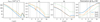 |
Fig. 1 Optical properties for three dust models. From left to right: the opacity per unit gas mass, assuming a gas-to-dust mass ratio of 100 (κext;λ); the scattering albedo ωλ; the forward throwing parameter gλ; and the polarization for the scattering angle of 90°. The gray vertical solid lines indicate three representative wavelengths for our calculations (3.5, 4.8, 12 μm; see text for details). The gray vertical dashed line indicates the wavelength for H band, for which we used imaging polarimetry to model the images for longer wavelengths. The dust opacity κext;λ is shown for the optical to mid-infrared wavelengths, while the remaining parameters for scattered and thermal emission are shown for near- to mid-infrared. The variations of optical properties at λ ~ 3 and ~10 μm are due to water ice and silicate, respectively. |
3 Equations to derive intensity distributions
3.1 Overview
In this section, we derive the equations to calculate the intensity distributions for three wavelengths (λ = 3.5, 4.8, and 12 μm) using the PI distribution observed in H band (λ = 1.65 μm). We derived the equations for scattered light and thermal emission assuming the following origins for the extended emission: (1) an optically thick and geometrically thin disk (Sect. 3.2); and (2) an optically thin remnant envelope (Sect. 3.3). Optically thick and geometrically thin disks have actually been seen in many edge-on disks associated with normal YSOs (e.g., Watson et al. 2007, for a review). We note that, however, some numerical simulations suggest that the aspect ratio of the disk surface (z/r) can reach up to 0.8–0.9 for FUor disks (Liu et al. 2016; Dong et al. 2016).
The targets associated with an optically thick envelope are beyond the scope of this study. Such YSOs exhibit an outflow cavity illuminated by the central source at optical and/or near-infrared wavelengths (e.g., Padgett et al. 1999). Such a reflection nebula is actually observed toward one of the FUor-like stars (Kóspál et al. 2008). We limit the applicability of our study to classical FUors, which do not show evidence for such optically thick envelopes with outflow cavities (Liu et al. 2016; Takami et al. 2018; Laws et al. 2020).
We assume that, at the radii of our interests (r > 10 au), the disk or the envelope is heated by the radiation from the central illuminating source. In practice, adiabatic heating or spiral shocks would significantly heat up gravitationally unstable disks, enhancing mid-infrared emission (e.g., Ilee et al. 2011; Vorobyov et al. 2020, 2022).
The viewing angle of the disk or the envelope, which affects the observed emission distribution, is uncertain, as the observed near-infrared intensity distributions are so complicated that they do not show a circular or elliptical distribution as observed for many disks associated with normal YSOs (Liu et al. 2016; Takami et al. 2018; Laws et al. 2020, – see also Sects. 1 and 4). High-resolution millimeter observations using ALMA can be useful for such measurements in some cases, in particular for disks associated with pre-main sequence stars (e.g., Long et al. 2018). However, the millimeter emission associated with FUors is often very compact, comparable to the angular resolutions of the ALMA observations (e.g., Cieza et al. 2018; Kóspál et al. 2021), perhaps due to emission in the inner disk region enhanced by viscous heating (Takami et al. 2019). As many of the near-infrared images for FUors do not show any evidence for large viewing angles, we assumed their viewing angles i to be ≲45° throughout our calculations.
In Sect. 3.4, we extend the equations adding the effect below. First, the central illuminating source may be either a compact self-luminous accretion disk (e.g., Hartmann & Kenyon 1996; Audard et al. 2014, for reviews) or a star (e.g., Herbig et al. 2003; Elbakyan et al. 2019). We derived equations for both cases, simultaneously correcting the fluxes and intensities for foreground extinction. In Sect. 3.5, we derive the equations to check self-consistencies of the calculations. In Table 1, we summarize major parameters used in the following subsections.
3.2 Emission from an optically thick and geometrically thin disk
3.2.1 Overview
We extended the approximation developed by Chiang & Goldreich (1997) and Chiang et al. (2001), and discussed in Dullemond et al. (2007). A disk consists of a geometrically thin surface layer and an optically thick disk interior, as shown in light and dark gray in Fig. 2. Throughout the paper, z is the coordinate perpendicular to the disk midplane; (x, y) is the coordinate parallel to the disk midplane; and r is the distance to the central source projected to the disk midplane  .
.
The optical thickness of the surface layer is about 1 along the light path to the central source, and significantly below 1 across the disk surface. Such a disk geometry was verified using realistic radiative transfer simulations with conventional models for circumstellar disks (e.g., Cotera et al. 2001; Takami et al. 2013), and multiwavelength imaging observations for some edge-on disks (e.g., Cotera et al. 2001; Grosso et al. 2003). As shown in these studies, the disk tends to have a large gradient in the optical thickness across its surface, and as a result, the location of the surface layer is relatively independent of wavelength. Throughout the paper, we approximated that the location of the disk surface is the same at all the wavelengths (optical to the mid-infrared; Sect. 4.1) for our calculations. Chiang & Goldreich (1997, 1999) and Chiang et al. (2001) successfully reproduced the observed spectral energy distributions (SEDs) for some YSOs with disks using this approximation.
For the following subsections we derived the equations for the following four emission components: (a) direct scattered light of the star via the surface layer (single scattering; Sect. 3.2.2); (b) light scattered from the surface layer toward the disk interior, and re-scattered in the disk interior toward the outside (double scattering; Sect. 3.2.3); (c) thermal emission from the surface layer (Sect. 3.2.4); and (d) thermal emission from the disk interior (Sect. 3.2.5). Figure 2 shows the schematic views for these components.
Full numerical radiative transfer simulations for optically thick dust disks often include the presence of an inner disk edge that can receive stellar light. This physical process would significantly increase the temperature of the entire disk (e.g., Whitney et al. 2003b; Robitaille 2011). We assumed that this radiative heating is negligible for the reasons below. It has been suggested that the FUors are associated with an optically thick compact ionized disk inside the dust disk (e.g., Hartmann & Kenyon 1996; Zhu et al. 2008). Such a disk can block stellar light toward the inner wall of the dusty disk.
Major parameters.
3.2.2 Single scattering
The intensity is approximately described as:
 (1)
(1)
 (2)
(2)
where Fλ(x, y) is the flux density of illumination by the central source for a unit area perpendicular to the direction of the incident light; ωλ is the scattering albedo; i is the viewing angle of the disk; P1(λ;θsca(x,y,i)) is the scattering phase function of the dust grains; θsca(x, y, i) is the scattering angle; and β(x, y) is the radial grazing angle of the disk surface with respect to the incident light from the central illuminating source. Equation (1) implies that the light observed via single scattering is a product of the light that the surface layer received from the star Fλα, the efficiency of scattering ωλP1, and an enhancement for the observations due to the viewing angle 1/cos i.
To accurately estimate the last term, we need to use the viewing angle of the disk surface with respect to line of sight of the observations rather than i. The alternative use of 1/cos i allowed us to reasonably simplify the calculations, but it is accurate only if the disk surface is nearly parallel to the disk midplane. In Sects. 3.5.1 and 4, we investigate how this simplification affects the accuracies of our calculations.
As described in Sect. 3.1, we assumed the viewing angle of the disk i to be ≲45°. Therefore, the 1/cos i term also yielded changes in the intensities of ~30%; this is significantly smaller than other uncertainties and systematic errors discussed later.
For the polarized intensity in H band, Eq. (1) is revised to:
 (3)
(3)
where P2 is the scattering phase function of the dust grains multiplied by the degree of polarization. For the polarization intensity, this single scattering component dominates the observations. The emission via multiple scattering is significantly fainter for the reason given below, as demonstrated using numerical simulations by Takami et al. (2013). For small grains, for which photons are fairly isotropically scattered, the scattered photons are polarized with a variety of position angles, canceling each other out. For large grains, which scatter most of the photons forward (that is with small θsca), the polarization of the individual photons is significantly reduced after the first scattering (see, e.g., Fig. 6 in Takami et al. 2013). Takami et al. (2013) executed radiative transfer calculations using more realistic disk models, which yielded an upper limit of the contribution of multiple scattering of 10% of the observed PI distribution.
Therefore, we replaced (PI)a;H(x, y) in Eq. (3) by (PI)obs;H(x, y), which is the observed PI distribution in H band, and derived the following equation:
 (4)
(4)
Using Eqs. (1) and (4) we derived:
 (5)
(5)

The scattering angle θsca depends on the viewing angle i, which is uncertain as discussed above. Furthermore, this angle is not exactly the same at the individual positions (x, y) of the disk: these are smaller and larger at the near and far sides of the disk, respectively. To avoid complexities, we used a representative constant for  defined below for each dust model:
![$ {a_\lambda } = \exp \left[ {0.5\left( {\log \;{a_{\lambda ;\min }} + \log {a_{\lambda ;\max }}} \right)} \right], $](/articles/aa/full_html/2023/11/aa45760-22/aa45760-22-eq12.png) (7)
(7)
where aλ;min and aλ;max are the minimum and maximum values measured at θsca = 45°–135°. Replacing  in Eq. (5) by aλ in Eq. (7), we derived:
 (8)
(8)
Figure 3 shows  for individual dust models at 3.5, 4.8 and 12 μm. We derived the phase function
  using the Henyey-Greenstein approximation. To derive P2(H; θsca), we used the approximation described below. We first derived the degree of polarization at θsca = 90° using the dust parameter files for HO-CHUNK, interpolating the value for the target wavelengths using scipy.interpolate.interpld. We then scaled the sine function using this value to derive the degree of polarization, and multiplied it by the Henyey–Greenstein function. The same approximation is also used for the HO-CHUNK radiative transfer code (Whitney et al. 2003b, Sect. 2). Takami et al. (2013) executed accurate calculations for the degree of polarization using the Mie theory, and showed that this approximation works well (see their Fig. 6).
In Fig. 3, the parameter  varies around the representative constant aλ by a factor of 1.3–1.4, 1.3–1.6, and 1.9–2.2 for λ = 3.5, 4.8 and 12 μm, respectively, at scattering angles of 45°–135°. We regard these factors as possible systematic errors in the calculated intensity distributions.
The range of scattering angles to derive aλ was selected based on the viewing angle of the disk (i ≲ 45°) discussed in Sect. 3.1. In practice, the height of the disk surface from the mid-plane makes the scattering angles smaller. Figure 3 shows that aλ;min and aλ;max derived above are actually valid for scattering angles as small as 10°–20°. Therefore, the adopted approximation would be valid unless the disk does not include extremely small scattering angles in the near side of the disk.
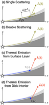 |
Fig. 2 Simplified disk geometry with a surface layer and the disk interior. The panels a–d explain the four emission components we discuss in Sect. 3.2.2–3.2.5, respectively. The green arrows indicate scattering of the stellar light at the wavelength of the observations. The blue arrows indicate the stellar light responsible for heating the surface layer and the disk interior. The red arrows indicate thermal emission from the surface layer and the disk interior. In the top panel, β is the radial grazing angle of the disk surface with respect to the incident light from the central illuminating source; δ is the radial inclination angle of the disk surface with respect to the midplane; and θ is the scattering angle. |
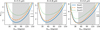 |
Fig. 3
|

3.2.3 Double scattering
We estimated the intensity distribution via double scattering on small grains using the following equation:
 (9)
(9)
The first, second, and third terms in the middle of the equation correspond to the light scattered at the surface layer into the disk interior, the scattering in the disk interior toward the outside, and an enhancement due to the viewing angle, respectively. The first term implies that half of the scattered light at the surface layer goes to the disk interior. For the second term, we approximated that the scattering occurs isotropically. As described in Sect. 3.2.2, the validity of this approximation was demonstrated by numerical simulations for polarized intensity by Takami et al. (2013).
We derived α(x, y) using Eq. (4) as:
 (10)
(10)
Figure 4 shows P2(H; θsca) for the three dust models. As for Sect. 3.2.2, we derived the representative constants as:
![$ {P_2}\left( H \right) = \exp \left\{ {0.5\left( {\log \left[ {{P_2}{{\left( H \right)}_{\min }}} \right] + \log \left[ {{P_2}{{\left( H \right)}_{\max }}} \right]} \right)} \right\}, $](/articles/aa/full_html/2023/11/aa45760-22/aa45760-22-eq21.png) (11)
(11)
where P2(H)min and P2(H)max are the minimum and maximum values measured at θsca=45°–135°. In this range of scattering angles, P2(H; θsca) varies by up to a factor of ~2 in terms of the representative constant P2(H). As for aλ;min and aλ;max in Sect. 3.2.2, P2(H)min and P2(H)max derived in this range of scattering angle is valid for small scattering angles caused by the height of the disk surface, down to θscat = 3°–8°.
Replacing P2(H; θsca) in Eq. (10) by P2(H), we derived:
 (12)
(12)
Substituting this equation to Eq. (9), we derived:
 (13)
(13)
Equation (13) shows that Ib;λ(x, y) is identical to Ia;λ(x, y) but with a different intensity level.
For scattering with large grains, for which forward scattering dominates, the scattered light would be propagated mainly along the disk surface, and faint in the other directions including those toward the disk interior. As a result, the contribution of Ib;λ(x, y) is smaller than the case with small grains. We therefore used Ib;λ(x, y) described in Eq. (13) as an upper limit.
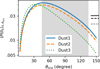 |
Fig. 4 P2(H; θsca) for different dust models. The black solid, dashed and dotted lines at the right side of the panel are the representative constants P2(H) derived using Eq. (11). The gray boxes show the range of the angles used to determine P2(H) (see the text for details). |
3.2.4 Thermal emission from the surface layer
The observed intensity would be described as follows:
 (14)
(14)
where τλ(x, y) is the optical thickness of the surface layer perpendicular to the disk plane; is the blackbody function; and Ts(x, y) is the temperature of the surface layer. Substituting Eq. (12) to Eq. (14), we derived:
 (15)
(15)
The temperature Ts(x, y) is derived using the following equation for the thermal budget of the surface layer:
 (16)
(16)
The left and right sides of the equation correspond to the total energies radiating in and out, respectively. Substituting Eq. (12), we derived:
![$ \matrix{ {\int {\left( {1 - {\omega _\lambda }} \right){B_{\lambda ,{T_{\rm{s}}}\left( {x,y} \right)}}} {\rm{d}}\lambda } \hfill \cr {\quad \quad \quad \~{{\cos \;i} \over {4\pi {\omega _H}{F_H}\left( {x,y} \right){P_2}\left( H \right)}}\left[ {\int {\left( {1 - {\omega _\lambda }} \right){F_\lambda }\left( {x,y} \right){\rm{d}}\lambda } } \right]} \hfill \cr {\quad \quad \quad \;\; \times {{\left( {PI} \right)}_{{\rm{obs}};H}}\left( {x,y} \right).} \hfill \cr } $](/articles/aa/full_html/2023/11/aa45760-22/aa45760-22-eq27.png) (17)
(17)
3.2.5 Thermal emission from the disk interior
The observed intensity would be described as follows:
 (18)
(18)
where Td(x, y) is the temperature of the disk interior just below the surface layer.
To derive Td(x, y), we considered the thermal budget as follows: half of radiation reaching to the surface layer is scattered or reemitted toward the disk interior, while the remain half escapes in the opposite direction (Chiang & Goldreich 1997); Chiang et al. 2001; Dullemond et al. 2007). We approximated that all the former radiation is absorbed in the disk interior. The thermal radiation from the disk interior escapes only outside of the disk. Therefore:
 (19)
(19)
where the left and right sides of the equation correspond to total energies radiating in and out, respectively. Substituting Eq. (12), we derived:
![$ \matrix{ {\int {\left( {1 - {\omega _\lambda }} \right){B_{\lambda ,{T_{\rm{d}}}\left( {x,y} \right)}}} {\rm{d}}\lambda } \hfill \cr {\quad \~{{\cos \;i} \over {2\pi {\omega _H}{F_H}\left( {x,y} \right){P_2}\left( H \right)}}\left[ {\int {{F_\lambda }\left( {x,y} \right){\rm{d}}\lambda } } \right]{{\left( {PI} \right)}_{{\rm{obs}};H}}\left( {x,y} \right).} \hfill \cr } $](/articles/aa/full_html/2023/11/aa45760-22/aa45760-22-eq30.png) (20)
(20)
In practice, some radiation from the disk surface toward the disk interior is not absorbed but scattered toward the outside of the disk, implying that the right side of Eq. (20) should be smaller to some extent than described. As a result, the temperature, and therefore Id;λ derived using Eq. (18) were overestimated to some extent.
3.3 Emission from an optically thin envelope
We considered radiative transfer processes similar to (a) and (c) shown in Fig. 2 and discussed in Sects. 3.2.2 and 3.2.4. If the envelope is geometrically thin, the emission via single scattering is described as:
 (21)
(21)
where κext;λ is the dust opacity; and Σenv(x, y) is the column density of dust associated with unit area of the envelope. This equation is the same as Eq. (1) for the surface layer of the disk, but α(x, y) is replaced by κext;λ∑env(x, y). In reality, the radiation field at the individual positions in the envelope Fλ(x, y) is also a function of z. We used a representative value over z (hereafter zenv) to reasonably simplify the calculations (Sect. 3.4).
Applying calculations similar to those in Sects. 3.2.2 and 3.2.3, we derived:
 (22)
(22)
 (23)
(23)
 (24)
(24)
The thermal emission from the optically thin envelope is described as:
 (25)
(25)
Substituting Eq. (23) we derived:
 (26)
(26)
We derived the temperature Te(x, y) using the following equation:
 (27)
(27)
The left and right sides of the equation correspond to the energy radiating out and in, respectively.
If the envelope is geometrically thick, one may want to remove the 1/cos i term from the above equations. This does not affect Eqs. (24), (26) and (27), as the term has been canceled out. Furthermore, the term was canceled out when we used Eq. (23) in Sect. 3.5.2. Therefore, we can use the same equations for a geometrically thick envelope as well.
3.4 Radiation from the illuminating source
3.4.1 Overview
In Sects. 3.2 and 3.3, we derived the equations for the individual emission components as functions of Fλ(x, y), that is radiation field by the central illuminating source at individual positions. In this subsection, we will replace them using the observed flux for the central source, considering the fact that the illuminating source is either a star or a flat compact self-luminous disk.
If the illuminating source is a star, the radiation of which is isotropic, the radiation field Fλ is approximately described for a geometrically thin disk or envelope as follows:
 (28)
(28)
where Fobs,λ is the observed flux from the central illuminating source; d is the distance from the observer to the target; and fλ is a factor to correct the foreground extinction, which is defined as:
 (29)
(29)
where Aλ is the extinction at the wavelength λ (Spitzer 1978). Throughout the paper, we derived Aλ/AV using the opacity for the ‘Dust2’ model for molecular clouds (Sect. 2). As a result, Eq. (29) could alternatively be described as follows:
![$ {f_\lambda } = \exp \left[ { - 0.921{A_V}{{\left( {{{{\kappa _{{\mathop{\rm ext}\nolimits} ,\lambda }}} \over {{\kappa _{{\mathop{\rm ext}\nolimits} ,V}}}}} \right)}_{{\rm{Dust}}2}}} \right], $](/articles/aa/full_html/2023/11/aa45760-22/aa45760-22-eq40.png) (30)
(30)
where (κext,λ/κext,V)Dust2 is the dust opacity normalized to that of the V band (λ = 0.55 μm) based on the ‘Dust2’ model. We assumed that there is no extinction between the central illuminating source and the disk or the envelope as it is likely that the strong FUor winds blow up dust grains in these regions (Takami et al. 2019).
If the illuminating source is a flat compact disk, Eq. (28) is replaced with:
 (31)
(31)
where γ is the sine of the grazing angle of the flat inner disk from the observer and the extended disk or envelope, therefore
![$ \gamma = \sin \left[ {{{\tan }^{ - 1}}\left( {z/r} \right)} \right]. $](/articles/aa/full_html/2023/11/aa45760-22/aa45760-22-eq42.png) (32)
(32)
In reality, γ varies with position on the disk surface and in the envelope, but inclusion of this variation would make the calculations too complicated to derive the intensity distributions in a straightforward manner. Therefore, we used constant values for our calculations (0.1, 0.2, and 0.4; Sect. 4; hereafter  ), and investigate how this approximation affects the accuracy of our calculations.
The term 1/cos i in Eq. (31) is to correct the observed flux for the viewing angle of the flat compact disk. Due to the assumed flat nature (z ~ 0) of the compact disk, the term 1/cos i in this equation is free from the systematic errors discussed in Sect. 3.2.2. To discriminate between these two cases, we bracketed 1/cos i with γ for those originating from Eq. (31).
Liu et al. (2016) showed the SEDs observed for a few FUors, with the stellar continuum that the authors derived based on their model fitting of the entire SED using their radiative transfer simulations. For their simulations, the central illuminating source is a star, however, the infrared excess over the stellar continuum is apparent at λ ≳ 3 μm as the inner disk is heated by stellar radiation. Therefore we regarded the illuminating source as an inner disk at λ ≥ 3 μm.
3.4.2 Revised equations for intensities and temperatures
We revised Eqs. (8), (15), (17), (18), (20), (24), (26) and (27) by substituting Eqs. (28) and (31). We also applied foreground extinction to the observed polarized intensity distributions (PI)obs;H(x, y); the derived intensity distributions Ia;λ(x, y), Ic;λ(x, y), Id;λ(x, y), Ia′;λ(x, y), and Ic′;λ(x, y); and the observed flux of the central source Fobs,λ. We corrected these parameters for foreground extinction by multiplying fλ defined in Eq. (30).
For the case where the illuminating source is a star at λ < 3 μm, we substituted Eq. (28) to FH(x, y) for all of the above equations. We also substituted Eq. (28) to Fλ(x, y) in Eqs. (17), (20), (27) as the heating of the extended disk or envelope is dominated by illumination at λ < 3 μm (Sect. 4.1). In contrast, we substituted Eq. (31), that of a flat compact disk, to (8), (24) to derive the intensity distributions for single scattered light in mid-infrared wavelengths. As a result, the revised equations are:
 (33)
(33)
 (34)
(34)
 (35)
(35)
 (36)
(36)
 (37)
(37)
![$ \matrix{ {\int {\left( {1 - {\omega _\lambda }} \right){B_{\lambda ,{T_{\rm{s}}}\left( {x,y} \right)}}{\rm{d}}\lambda } } \hfill \cr {\;\~{{\cos \;i} \over {4\pi {\omega _H}{P_2}\left( H \right)}}\left[ {\int {\left( {1 - {\omega _\lambda }} \right)f_\lambda ^{ - 1}{F_{{\rm{obs}},\lambda }}{\rm{d}}\lambda } } \right]{{{{\left( {PI} \right)}_{{\rm{obs}};H}}\left( {x,y} \right)} \over {{F_{{\rm{obs}},H}}}},} \hfill \cr } $](/articles/aa/full_html/2023/11/aa45760-22/aa45760-22-eq49.png) (38)
(38)
![$ \matrix{{\int {\left( {1 - {\omega _\lambda }} \right){B_{\lambda ,{T_{\rm{s}}}\left( {x,y} \right)}}{\rm{d}}\lambda } } \hfill \cr {\;\~{{\cos \;i} \over {2\pi {\omega _H}{P_2}\left( H \right)}}\left[ {\int {f_\lambda ^{ - 1}{F_{{\rm{obs}},\lambda }}{\rm{d}}\lambda } } \right]{{{{\left( {PI} \right)}_{{\rm{obs}};H}}\left( {x,y} \right)} \over {{F_{{\rm{obs}},H}}}},} \hfill \cr } $](/articles/aa/full_html/2023/11/aa45760-22/aa45760-22-eq50.png) (39)
(39)
 (40)
(40)
If the central source is a self-luminous disk, we alternatively substituted Eq. (31) to FH(x, y) and Fλ(x, y) for all equations. As a result, we replaced Eqs. (33), (34), (36), (37) and (40) with the following equations:
 (41)
(41)
 (42)
(42)
 (43)
(43)
 (44)
(44)
 (45)
(45)
We used these equations together with Eqs. (7), (11), (13) for aλ, (P2)H, and Ib;λ(x, y), respectively, to derive the intensity distributions. As shown in Eqs. (33), (36), (41) and (43), Ia;λ(x, y) and Ia′;λ(x, y) (therefore Ib;λ(x, y) as well; see Sect. 3.2.3) are identical to PIobs;H(x, y) but with different intensities levels under the given approximations of scattering angles made in Sects. 3.2.2 and 3.2.3.
3.5 Checking self-consistencies
In this subsection we derive the equations to check self-consistencies of calculations for an extended disk (Sect. 3.5.1) and an envelope (3.5.2).
3.5.1 Surface geometry of the extended disk
We summarize below the approximations which can potentially cause significant systematic errors, among those we used in previous subsections:
- (A)
We multipled the intensities by 1/cos i, where i is the viewing angle of the disk midplane, for the enhancement of the intensity, ignoring the inclination of the disk surface from the midplane at individual positions (Sect. 3.2.2).
- (B)
We derived Eqs. (28) and (31), omitting the term for the height of the disk surface from the midplane or the vertical distribution of the envelope (Sect. 3.4).
- (C)
We used a representative constant
 , without including its spatial variation (Sect. 3.4).
In this subsection, we derive the equations to investigate this. We first discuss the case that the central illuminating source is a star. Substituting Eq. (28) to Eq. (12), and also correcting foreground extinction for (PI)obs;H, we derived:
 (46)
(46)
As defined in Eq. (2), α(x, y) must range between 0 and 1.
We derived the inclination of the disk surface δ(x, y) in the radial direction in terms of the disk midplane, and its height from the disk midplane as:
![$ \matrix{ {\delta \left( {x,y} \right)} \hfill & { = {{\tan }^{ - 1}}\left[ {{z_{{\rm{disk}}}}\left( {x,y} \right)/r} \right] + \beta \left( {x,y} \right)} \hfill \cr {} \hfill & { = {{\tan }^{ - 1}}\left[ {{z_{{\rm{disk}}}}\left( {x,y} \right)/r} \right] + {{\sin }^{ - 1}}\alpha \left( {x,y} \right),} \hfill \cr } $](/articles/aa/full_html/2023/11/aa45760-22/aa45760-22-eq59.png) (47)
(47)
 (48)
(48)
The integrations in Eq. (48) would be made from the central source toward all the position angles. In practice, the central illuminating source is extremely bright compared with the extended emission, making the observations of the PI distribution close to the central source unreliable (Liu et al. 2016; Takami et al. 2018; Laws et al. 2020, see Sect. 4). Therefore, we alternatively executed the integration as follows:
 (49)
(49)
where  is the height of the disk surface at the outer edge of the software aperture mask at the central source, which is a free parameter. We cannot constrain this parameter from the observations (Takami et al. 2014). The adopted
  and calculated zdisk(x, y) must be approximately consistent with
  defined and used in Sect. 3.4. In Sect. 4.2, we adjusted
  to investigate whether self-consistent solutions exist.
If the central illuminating source is a compact self-luminous disk, we replaced Eq. (46) with the equation below, using Eq. (31) instead of Eq. (28):
 (50)
(50)
We calculated zdisk(x, y) and δdisk(x, y) by substituting this equation to Eq. (47) and execute numerical integrations with Eq. (49).
For some cases, the calculated values of α(x, y) and δ(x, y) exceed 1 and 90°, respectively (Sect. 4.2). In these cases, we conclude that the given combination of the SED, the central source and the dust model is not consistent with the PI distributions in H band.
3.5.2 Optical thickness of the extended envelope
We checked optical thicknesses for the following two directions: the radial direction (τr;λ); and the line of sight to the observer, that is:
 (51)
(51)
Substituting Eqs. (23), (28) and (31), and also correcting foreground extinction for (PI)obs;H, we derived the following equations in the cases that the central illuminating source is a star and a flat compact disk, respectively:
 (52)
(52)
 (53)
(53)
Suppose that, at each of the (x, y) positions, the dust grains are vertically and uniformly distributed up to a height twice the typical value zenv(x, y). We would then be able to estimate τr;λ as:
 (54)
(54)
As  (Eq. (32)), we revised this equation as:
 (55)
(55)
We regard this value as a typical optical thickness in the radial direction. As for Eq. (49), the integrations were made for all the position angles. The equation yields a lower limit of the actual optical thickness as we cannot include the opacities within rmin.
Targets.
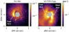 |
Fig. 5 PI distribution in H band, PIobs;H, for FU Ori and V1735 Cyg (Takami et al. 2018), with a pixel scale of 9.5 mas, normalized to the Stokes I flux of the central source. North is up. In each image, the central region is masked as we were not able to make reliable measurement due to the central source being significantly brighter than the extended emission. Features such as spiral arms are labeled (see the text for details). |
4 Application
In this section, we apply the equations in Sect. 3 to two FUors: FU Ori and V1735 Cyg. We summarize the properties of these objects in Table 2. For H band imaging polarimetry, we used the images obtained using Subaru-HiCIAO by Takami et al. (2018). As shown in Fig. 5, each object is associated with (1) a bright arm-like feature or two; and (2) surrounding diffuse extended emission. As discussed in Sect. 1, we regard the former as the features of our major interest for understanding the accretion process onto FUors.
In Sect. 4.1, we describe radiation from the central source. In Sect. 4.2, we check self-consistencies for the individual cases using the equations derived in Sect. 3.5. In Sect. 4.3, we investigate the individual emission components, and show that the intensity distribution is dominated by the single scattering process for all the cases. In Sect. 4.4, we present the distributions for the single-scattering emission for all the cases, compare their intensities, and further discuss their self-consistencies.
We executed calculations for  , 0.2 and 0.4. In Sects. 4.2–4.4 we mainly present the results for
  , and briefly summarize the results for the cases with
  and 0.4. We present the detailed results for the latter cases in Appendix A.
We executed all the calculations using numpy and scipy for a viewing angle i=0° (that is the face-on view). If the extended emission is due to a disk with an intermediate viewing angle (i ~ 45°), we would expect scattered emission from not only the front side of the surface, but also the edge of the opposite side with a dark lane in between (e.g., Watson et al. 2007; Liu et al. 2016; Dong et al. 2016). The H band images at a large field of view do not show evidence for the latter emission component (Liu et al. 2016; Takami et al. 2018; Laws et al. 2020), supporting the idea of a small viewing angle. For the case that the extended emission is due to an optically thin envelope, we will discuss in Sect. 4.5 how the use of an intermediate viewing angle affects the results.
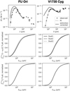 |
Fig. 6 Radiation from the central sources. Top: The spectral energy distributions. The crosses show the observations; the dotted curves show fittings; and the solid curves show those corrected for foreground extinction. Middle: Cumulative fraction of the integrations used in Eqs. (38), (40) and (45). The horizontal axis is the maximum wavelength for integration up to λ=15 μm. Bottom: Same as the middle panels but for the integrations used in Eq. (39). |
4.1 Illumination by the central source
We derived the SEDs for these targets using fluxes collected from the literature by Gramajo et al. (2014). The observations were made using the Infrared Astronomical Satellite (IRAS), the Infrared Space Observatory (ISO), the Midcourse Space Experiment (MSX), the Kuiper Airborne Observatory (KAO), the Balloon-borne Large Aperture Submillimeter Telescope (BLAST), the James Clerk Maxwell Telescope (JCMT) and various ground-based telescopes for optical to mid-infrared wavelengths. These data cover the wavelength ranges of 0.55–850 μm and 1.24–500 μm for FU Ori and V1735 Cyg, respectively, at angular resolutions up to ~3′. For V1735 Cyg, we added the optical fluxes measured by the Sloan Digital Sky Survey (SDSS) project for the g (0.47 μm, 20.7 mag), r (0.62 μm, 17.4 mag), i (0.75 μm, 15.2 mag), and z bands (0.89 μm, 13.4 mag).
In Fig. 6, we show the observed SEDs, the fitting curves obtained using scipy.interpolate.interpld, and those curves after correcting for the foreground extinction tabulated in Table 2. The observed SEDs show a remarkable far-infrared excess at λ > 15 μm, which is due an envelope, not the central illuminating source (e.g., Gramajo et al. 2014). We therefore obtained the fitting curves at up to λ =15 μm for the integrations with the central illuminating source in Eqs. (38), (39), (40) and (45). For the shortest wavelengths, we extrapolated the curves down to λ = 0.3 μm using the same python command. In Table 2, we show the source luminosities obtained using these curves.
In Fig. 6, we also show the cumulative fraction for the integrations at the right side of Eqs. (38), (39), (40) and (45) as a function of the maximum wavelength. The curves in the middle and bottom panels of the figure indicate that the flux at λ < 3 μm is responsible for ~90% of radiative heating by the central illuminating source for FU Ori, and 70–80% for V1735 Cyg, agreeing with the calculations we made in Sect. 3.4.
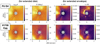 |
Fig. 7 Parameters for disks and envelopes derived from the H band images. From left to right: the aspect ratio for the surface of the extended disk; the radial inclination angle for the surface of the extended disk; the optical thickness of the extended envelope in H band (λ = 1.65 μm) from the central star in the radial direction; the same but for line of sight of the observations. The calculations are made for |

Disk surface aspect ratio zdisk/r at the minimum radius r = rmin.
4.2 Self-consistencies
4.2.1 Cases illuminated by a star
Table 3 shows the disk surface aspect ratio zdisk/r at r = rmin (that is at the edges of the software mask as the center) used for the integration of Eq. (49). These values were adjusted to minimize deviation of γdisk(x, y) from the representative constant  for most of the region. Figure 7 shows the aspect ratio and the radial inclination angle of the disk surface, derived assuming that the observed extended emission is associated with a disk; and the optical thickness for H band in the radial direction and line of sight, derived assuming that the observed extended emission is associated with an envelope. The ‘Dust1’ model is used to derive all the images.
All the calculated images show that the values are small, agreeing with the assumptions and approximations used in Sect. 3. In Fig. 7, the east arm from FU Ori and the tip of the west arm from V1735 Cyg significantly increase zdisk, δ and τr;H in the outer regions. The figure also show relatively large τl;H for these bright features seen in the PI distribution in H band.
Figure 8 shows the distributions of pixel values for γdisk(x, y) for the individual cases. These show relatively small ranges around the representative constant  , within 25% for most of the regions. This implies that the amplitudes of the variation of the disk surface is significantly smaller than the height of the disk surface, as shown by analysis and numerical simulations for some protoplanetary disks (Takami et al. 2014; Zhu et al. 2015).
These trends are the same for different targets and dust models. In Table 4, we tabulate the maximum values for the parameters shown in Fig. 7, and the standard deviation for γdisk from the representative constant  . We find the same trends, that support the self-consistency, for
  are 0.4 as well (Appendix A.1).
4.2.2 Cases illuminated by a flat compact disk
Figures 9 and 10 are the same as Figs. 7 and 8 but with a flat compact disk as the illuminating source, and  . We derived the parameters for the extended disks in these figures assuming zdisk/r = 0.01 at r = rmin. In Fig. 9, the images for zdisk/r and δ have variations significantly larger than the case with a star as the central source shown in Fig. 7. Figure 10 shows that γdisk(x, y) also has large variation from
  , by a factor of more than 2 in 21–35% of the region.
During the integration using Eqs. (47) and (49), δ(x, y) becomes 90° or larger in the left side of FU Ori and the bottom-left corner of the images for V1735 Cyg, making the integration in the outer regions impossible. As discussed in Sect. 3.5.1, this implies that the given combinations of the central source and the dust model cannot explain the observed PI distribution in these regions. In some of these regions, α(x, y) also exceeds 1, inconsistent with its definition with Eq. (2).
Figure 9 also shows that the optical thickness of the extended envelope is significantly larger than the case with a star as the central source shown in Figs. 7, by the factor  as shown in Eq. (53). In some regions, the optical thickness exceeds 0.7, implying that self-absorption in the envelope reduces the emission from the central source or toward the observer by a factor of ~2.
In Sect. 4.4, we further investigate the self-consistencies of the calculations for different cases for  . For
. For  , we were able to obtain self-consistent results for all the cases. For
  , we were able to obtain self-consistent results for the bright part of the east and west arms for V1735 Cyg, for the cases that the extended emission is due to an envelope. See Appendix A.2 for details.
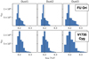 |
Fig. 8 Histograms for γdisk for the case with a star as the central illuminating source. The vertical axis shows the number of pixels for each bin. The vertical dashed line in each panel shows the representative constant |

Parameters for surface geometry of disks and optical thicknesses of envelopes.
Upper limit intensity ratios for the double-scattering emission per single-scattering emission.
4.3 Individual emission components
Figures 11 and 12 show the individual emission components for FU Ori at λ = 12 μm, assuming that the extended emission is due to a disk and an envelope, respectively. The calculations were made for  with a combination of a star as the central illuminating source and the ‘Dust1’ model. For thermal emission, we set the minimum temperature of the disk and the envelope to be 30 K. The fraction of the thermal emission to the total emission is largest for the selected wavelength (that is the longest wavelength).
Under the given approximation, the intensity distributions for scattered emission Ia(x, y), Ib(x, y) and Ia′(x, y) are identical to that of the PI distribution (Sects. 3.2.3 and 3.4.2). In Table 5, we show the Ib(x, y)/Ia(x, y) intensity ratios calculated using Eq. (13). As shown in the table, Ib(x, y) is fainter than Ia(x, y) by a factor of 5 or larger. As discussed in Sect. 3.2.3, the calculated Ib(x, y) may be overestimated, therefore the actual contribution of the double scattering emission to the total intensity may be even smaller.
Figures 11 and 12 show that the thermal emission components Ic, Id, and Ic are significantly fainter than the single scattering emission, at least by a factor of 100 for most of the regions. This is due to the low temperatures (T ≲ 70 K) derived in these regions. In Table 6, we list the maximum intensity ratios for thermal emission divided by the single scattering emission for a variety of cases. The table shows a maximum value of 0.25 for V1735 Cyg at λ =12 μm, with the ‘Dust1’ model and a star as the illuminating source, and for the case where the extended emission is due to an envelope. Even in this case, the ratio is below 0.03 for more than 98% of the region. For the remaining cases, the tabulated maximum intensity ratios are 0.08.
Table 7 shows the minimum fraction of the single scattering emission to the total intensity. The table shows that the single scattering emission is responsible for more than 80% of the total intensity for all cases and positions. This emission component does not significantly suffer from the possible large systematic errors (A), (B) and (C) discussed in Sect. 3.5.1 for the extended disks, as explained below. For (A), the equations for single-scattering emission (33), (41) do not include cos i that can cause large systematic errors. The cos i terms with  in the former equation can yield a systematic error only up to ~30% (Sects. 3.2.2 and 3.4.1). The term for (B) has been canceled out in Eqs. (33) and (41) as this effect equally affect the observed PI distribution in H band and modeled mid-infrared emission. For (C),
  is included in Eq. (33) for which the illuminating source is a star. Therefore, the spatial variation of γdisk(x, y) from the representative constant
  is relatively small (<25% for most of the pixels; Sect. 4.2.1).
For the case that the extended emission is due to an envelope, some regions suffer from large optical thickness (τ ≳ 0.7, corresponding to a degradation in the flux or intensity of a factor of ≳2), which we did not include when deriving the equations (Sect. 4.2.2). Fortunately, these are still small for the arm-like features (Sect. 4.4), that is the features of our major interest for investigating the mass accretion process (Sect. 1).
As described in the beginning of this subsection, all of the above calculations are made for  . The single-scattering emission dominates the total intensity distributions for
  and 0.4 as well (Appendix). We note that all the images for single scattering emission still suffer from an internal systematic error by a factor of up to ~2, based on the simplification aλ (Sect. 3.2.2) made to avoid the complexity of calculations with a variety of scattering angles.
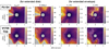 |
Fig. 9 Same as Fig. 7 but with a flat compact disk as the central illuminating source and the ‘Dust3’ model. The white dotted contours in the left two panels indicate the disk surface aspect ratio zdisk/r = 0.5 and the radial inclination of the disk surface δ = 30°, respectively, for the extended disk. The blue and black contours in the right two panels indicate the optical thicknesses τ = 0.35 and 0.7, respectively, in the extended envelope. The gray circle in each panel shows the area where we were not able to execute reliable calculations because of the bright central source in the PI image. The other gray areas indicate the regions where we have not been above to execute self-consistent calculations (see the text). |
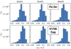 |
Fig. 10 Same as Fig. 8 but with a flat compact disk as the central illuminating source, and with a logarithmic scale for the horizontal axis. |
4.4 Single-scattering emission
Figures 13 and 14 show the intensity distributions for single-scattering emission at λ = 12 μm for FU Ori and V1735 Cyg, respectively, for all the cases which assumed that the central illuminating source is a flat compact disk, and  . As discussed above, all the images are identical to the PIdistribution in H band but with different intensity levels. As shown in Eqs. (41) and (43), the intensity is independent of the assumed
  for these cases.
In Fig. 13, the left (east) side of the east arm is masked for the case in which the extended emission is due to a disk with the ‘Dust3’ model, as the radial inclination of the disk surface δ exceeded 90° during the integration. This is caused by the emission of the bright part of the east arm. Following our discussion in Sect. 4.2.2, we conclude that the given conditions for this image are not consistent with the presence of this east arm, that is the major feature for this object. In the upper panels of Fig. 14, the masked regions for δ ≥ 90° are located in the left corner, and also the bottom edge of the image for the ‘Dust3’ model. This implies that the emission in these regions cannot be explained with an extended disk. It is still possible to attribute the emission in the inner region (including two arms) to an extended disk, and the outer region to an extended envelope.
In the bottom panels of Figs. 13 and 14, the optical thickness from the center or along the line of sight exceeds 0.7 (corresponding a decrease in the flux or intensity by a factor of ≳2) in H band in the hatched areas. When we derived the equations in Sect. 3, we assumed that the extended envelope is optically thin, and did not include the decreased intensities due to optical thickness. Therefore, the derived intensities are not very accurate in and near these regions, with a systematic error of a factor of ≳2. Fortunately, most of the emission associated with the arms does not suffer from this optical thickness issue.
If the central source is a star, the intensities are fainter by a factor of  as shown in Eqs. (33), (36), (41) and (43). All the results are self-consistent for these cases as discussed in Sect. 4.2.1. In the areas where the approximation works well, the intensity ratios are derived as follows using Eqs. (33), (36), (41) and (43):
 (56)
(56)
 (57)
(57)
Figure 15 shows the intensities normalized to that of an extended disk, a flat compact disk as the illuminating source and the ‘Dust1’ model. These intensity ratios are independent of the target object (FU Ori or V1735 Cyg). For each wavelength, the intensities range over a factor of 20–800, depending on the central illuminating source, whether the extended emission is due to a disk or an envelope, the dust models and the observing wavelengths (λ = 3–13 μm). The ranges are smaller for shorter wavelengths due to the smaller differences in dust properties from those for the H band.
The intensity ratio given by Eq. (57) is smaller than 1 at the target wavelengths (see Fig. 1), implying that the extended emission is fainter if it is due to an envelope. Therefore, the intensities in this case would be lower limits. In reality, the optically thinner nature for longer wavelengths may allow us to reveal the presence of an embedded disk even in the case that the emission observed in H band is dominated by an envelope, as described in Sect. 1.
Maximum ratios for thermal to single-scattering emission.
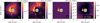 |
Fig. 11 Images for the individual emission components. From left to right: the single-scattering component (Ia); thermal emission from the surface layer (Ic) and the disk interior (Id); and the intensity ratio for the thermal emission (Ic+Id) per the single scattering emission for FU Ori at λ =12 μm, assuming that the extended emission is associated with a disk, and |

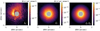 |
Fig. 12 Same as Fig. 11 but assuming that the extended emission is associated with an envelope. From left to right: Intensity distributions for the scattered emission |


Minimum fraction of single-scattering emission to total intensity.
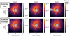 |
Fig. 13 Intensities for the single-scattering component for FU Ori at λ = 12 μm, for the cases where the extended emission is due to a disk (top) and an envelope (bottom), and for different dust models. The central illuminating source is assumed to be a flat compact disk. The white dotted contours in the upper panels are for the disk surface aspect ratio zdisk/r = 0.5; the white dotted contours in the lower panels are for the H band optical thickness in the radial direction τr = 0.35 and 0.7; and the black solid contours in the lower panels are for the H band optical thickness along line of sight τl = 0.35 and 0.7. The regions with τr>0.7 and τl>0.7 are hatched in the bottom-right panel. In the top-left panel, the left (east) side of the east arm is masked as the calculations are not self-consistent (see the text). |
4.5 Dependence on viewing angle
We made calculations in Sects. 4.2–4.4 for the viewing angle i=0°. As discussed in the beginning of the section, the viewing angle appears to be close to zero if the extended emission is due to a disk, however, it could be intermediate (i ~ 45°) if the extended emission is due to an envelope. As discussed in Sect. 4.3, this does not significantly affect the calculated single scattering emission, which dominates the total intensity distribution, as the terms with the viewing angle have been canceled out in Eqs. (36) and (43).
In contrast, an intermediate viewing angle would yield a larger r and a smaller Fλ(x, y) with Eqs. (28) and (31), and therefore a larger optical thicknesses for the extended envelope, for example, by a factor of 2–3 for i ~ 45° (see Eqs. (52)–(55). This would increase the areas where the calculated intensity distribution for the single scattering emission is not reliable. In Figs. 13 and 14, the figures obtained for i=0°, the regions with τl;H > 0.35 (therefore τl;H > 0.7–1 for i = 45°) cover significant fractions of the arm features for FU Ori with all the dust models, and V1735 Cyg with the ‘Dust3’ models. One would regard the calculated emission in these regions as not reliable for such a viewing angle. We emphasize that, however, the discussion in this subsection does not exclude a possibility that the disk or the envelope associated with these targets have a significantly smaller viewing angle, close to i=0°.
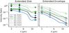 |
Fig. 15 Relative intensities for single scattering emission for various cases. All the values are normalized to that of an extended disk with the ‘Dust1’ model, with a flat compact disk as the illuminating source, and λ = 3.5 μm. The left and right panels are for the case where we assumed the extended emission is associated with a disk and an envelope, respectively, For each panel, we show the intensity ratios for different illuminating sources and dust models. |
5 Benchmark calculations with monochromatic radiative transfer simulations
One may be concerned that the approximations used to calculate the disk emission (Sect. 3.2) may significantly degrade the accuracy for our calculations. In this section, we perform monochromatic Monte-Carlo radiative transfer simulations using the Sprout code (Takami et al. 2013)2 and demonstrate how well the semi-analytic calculations using H band calculations reproduce the simulated images. We explain the method and show the results in Sect. 5.1. In Sect. 5.2, we briefly discuss what we need for full radiative transfer simulations to verify the calculations for the thermal emission components.
5.1 Method and results
As is common in some full radiative transfer codes (Whitney et al. 2003b; Robitaille 2011), we used the following equation for a flared disk (Shakura & Sunyaev 1973); Lynden-Bell & Pringle 1974):
![$ \rho \left( {r,z} \right) = {\pi _0}\left[ {1 - \sqrt {{{{R_0}} \over r}} } \right]{\left( {{{{R_0}} \over r}} \right)^\alpha }\exp \left\{ { - {1 \over 2}{{\left[ {{z \over h}} \right]}^2}} \right\}, $](/articles/aa/full_html/2023/11/aa45760-22/aa45760-22-eq106.png) (58)
(58)
where ρ0 is a constant to scale the density; R0 is a reference radius for ρ0; α is the radial density exponent; and h is the disk scale height. The scale height h increases with radius as h = h0(r/R0)β, where h0 is the disk scale height at the reference radius; β is the flaring power. As is also common in some models (Robitaille et al. 2006, 2007; Dong et al. 2012a; Takami et al. 2013), we assumed α = β + 1, which yields the surface density distribution Σ(r) ∝ r−1, approximately agreeing with that inferred from millimeter interferometry for disks associated with many low-mass pre-main sequence stars (Andrews et al. 2009, 2010). Use of an independent α is beyond the scope of this work.
Table 8 summarizes the parameter set we used for simulations. We used a disk mass of 0.1 M⊙ based on recent mini-survey observations of FUor disks using ALMA (Kóspál et al. 2021). Similar disk masses were also estimated by fitting the observed infrared spectral distributions for FUors using full radiative transfer simulations (Gramajo et al. 2014). The outer disk radius of 500 au was set based on the H band imaging polarimetry shown in Sect. 4. The inner disk radius was chosen to not let it block the light from the central source to the outer disk surface. Under this condition, this parameter does not affect the results significantly as long as it is located within the central mask for the H band image (Sect. 4). The selected β of 1.3 is comparable to that used for protoplanetary disks associated with normal YSOs (e.g., Dong et al. 2012a; Takami et al. 2013; Follette et al. 2015). The parameters ρ0 and h* were chosen to satisfy the given disk mass and  .
.
In this section we used the ‘Dust3’ model, which consists of astronomical silicate and graphite. The optical constants for the target wavelengths are obtained from Draine & Lee (1984). We note that different authors use different types of carbon dust, either graphite or amorphous carbon (Cotera et al. 2001; Wood et al. 2002). While graphite has been extensively used (e.g., Draine & Lee 1984; Laor & Draine 1993; Kim et al. 1994; Whitney et al. 2003b; Robitaille et al. 2006; Dong et al. 2012a,b), far-infrared SEDs of YSOs and evolved stars suggest the absence of graphite and presence of amorphous carbon in circumstellar dust (Jäger et al. 1998, and references therein). We used graphite for consistency with the dust parameter files used in earlier sections.
Following Sect. 3.4, we executed Monte-Carlo scattering simulations using this disk model for the following cases: (1) λ =1.65 μm for the case that the central illuminating source is a star; and (2) λ = 1.65, 3.5, 4.8 and 12 μm for the case that the central source is a flat compact self-luminous disk. We used 5×10⁸ photons for each case. Each photon was initially ejected from the central source, which is approximated as a point source either for a star or a flat self-luminous compact disk. The photons were isotropically ejected from the central source for both cases. Each photon has a ‘weight’ corresponding to its Stokes I. The weights for all the initial photons are the same if the central source is a star. If the central source is a flat compact disk, we scaled the weight of the photons based on its grazing angle.
The light path for the next scattering position was calculated for the opacity distribution determined by Eq. (58), Table 8, and the dust opacity for the wavelength of the calculations. The scattering angle and the resultant Stokes parameters were calculated based on the Mie theory. The former was calculated using the ‘table look-up method’, which yields accuracies better than the Henyey-Greenstein approximation used in Sect. 3 (Fischer et al. 1994; Takami et al. 2013). We then scaled the photon weight by the scattering albedo, and continued the calculation until each photons escapes from the region of the interest. To save time for calculations, photons with more than ten scatterings were removed because of small photon weights, and therefore small contribution to the simulated images. The photons escaping out from the region of our interest were collected with ten image detectors for different viewing angles. Each detector consists of 101 × 101 pixels to sample the image of the entire disk. The partition of the viewing angles for the detectors was made to receive equal number of photons in the case that the radiation is isotropic. For face-on and intermediate viewing angles, we used the results for the photons integrated over the angles of 0°–26° and 37°–46°, respectively. See Takami et al. (2013) for other details of the simulations.
Figure 16 shows the τ =1 disk surfaces for κext = 3, 30, and 300 cm2 g−1. To derive the equations in Sect. 3.2, we have approximated that the location of the disk surface is the same for all the wavelengths of our interest shown in Fig. 1. Small differences in the locations of the disk surfaces in Fig. 16 justify this approximation. Figure 17 shows all the simulated images for the face-on (i = 0°–26°) and the intermediate viewing angle (37°–46°). While most of the emission is associated with the front side of the disk, we also find the emission from the edge of the back side of the disk in the bottom of each image, and a dark lane which corresponds to the outer disk edge. These features are prominent in the images for the intermediate viewing angle.
Using the simulated H band polarimetry at λ = 1.65 μm, we derived the images at 3.5, 4.8 and 12 μm using Eqs. (33), (41), and (13). In Fig. 18, we show these images divided by those directly obtained by monochromatic radiative transfer simulations (Fig. 17). Figure 19 shows the histograms of the intensity ratios for the individual cases. These histograms were made as follows. From the simulated images we first removed the emission associated with the dark lane and the back side of the disk. This is because the intensity ratios are significantly different from the front side of the disk surface, as shown in Fig. 18, but the actual observations in Fig. 5 does not clearly show the presence of such an outer disk edge. We then applied 5×5-pixel binning to increase the signal-to-noise before taking the intensity ratios.
In Figs. 18 and 19, the measured intensity ratios range between ~0.5 and ~2, implying that our new semi-analytic method yields intensities at an accuracy within a factor of ~2. Large values are observed for the longest wavelengths (λ=12 μm), as the actual disk surface is below that for λ=1.65 μm used for the semi-analytic calculations, making the numerical values smaller. Larger dispersions of the ratios for the intermediate viewing angle is due to a combination of a large variation of the scattering angles at the disk surface, and the use of a representative aλ defined with Eq. (6).
Disk parameters for the monochromatic Monte-Carlo radiative transfer simulations.
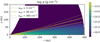 |
Fig. 16 Density distribution used for the monochromatic Monte-Carlo radiative transfer simulations. The green curves show the τ = 1 disk surfaces for κext = 3, 30, and 300 cm2 g−1. |
5.2 Toward full radiative transfer simulations
To better check our semi-analytic calculations, one may wish to see full radiative transfer simulations including radiation and viscous heating of the disk, to accurately calculate thermal emission. Such simulation codes include HO-CHUNK, HOCHUNK-3D (Whitney et al. 2003b, 2013) and Hyperion (Robitaille 2011). These codes can only place a star as the central source, not a compact self-luminous disk. The presence of such an optically thick ionized disk for FUors has been extensively discussed over many years (e.g., Hartmann & Kenyon 1996; Audard et al. 2014, for reviews). As discussed in Sect. 3.1, the absence of such a disk would also yield the following problem. The inner edge of the dust disk is exposed to stellar radiation, yielding temperatures in the disk significantly higher than calculated using our semi-analytic method. Therefore, we need to revise the existing codes for the above issues to perform comparisons with our semi-analytic calculations.
The typical disk model used in Sect. 5.1 yields a very large optical thickness in the inner radii. It therefore demands significant computational time due to the number of scatterings, absorptions and reemissions. Our trials with Hyperion, which includes algorithms to efficiently solve this problem, suggest the need of a cluster computer with several tens or hundred cores to obtain results with different mass accretion rates within a few days.
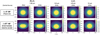 |
Fig. 17 Images obtained using monochromatic Monte-Carlo radiative transfer simulations. See text for details. |
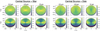 |
Fig. 18 Intensities derived using the new semi-analytic method, divided by those directly derived using monochromatic radiative transfer simulations. As for Fig. 17, the top and bottom panels show images for the face-on view (i=0°–26°) and the intermediate viewing angle (i=37°–46°), respectively. In each panel, the region below the white dashed curve, that are associated with the emission from the outer disk edge, show large variations. These regions were not included in our analysis to verify the calculations (see text for details). |
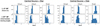 |
Fig. 19 Histograms for intensity ratios for Fig. 18 after applying 5 × 5 binning. The dashed vertical panel indicate an intensity ratio of 1. See text for details. |
6 Summary and discussion
We have developed a semi-analytic method to estimate the intensities of mid-infrared extended emission associated with FUors from the observed PI distributions in the H band (λ = 1.65 μm). The extended disk or envelope responsible for the infrared extended emission is illuminated by the central source, which is either a star or a flat compact self-luminous disk. For our calculations, we assumed that the disk or the envelope is radiatively heated. The disks associated with YSOs, including FUors, must be optically thick at optical to mid-infrared wavelengths. We approximated that an extended disk consists of a surface layer with an optical thickness of approximately one along the line of sight of the radiation from the central source, and an optically thick disk interior. We then calculated emission from extended disks for single scattering, double scattering, and thermal emission from the surface layer and the disk interior. For the envelope, we assumed that it is optically thin, and we derived the equations for single-scattering emission and thermal emission. We also derived equations to check consistencies of the calculations for the assumptions and the approximations we used.
We carried out the calculations for two FUors, FU Ori and V1735 Cyg, for three wavelengths (λ = 3.5, 4.8, and 12 μm), using three dust models and (1)  , 0.2, and 0.4, and (2) a viewing angle of zero (face-on). The near-infrared emission observed toward these targets supports the idea of the face-on view if the extended emission is due to a disk. The viewing angle may be intermediate (for example, i~45°) if the extended emission is due to an envelope, but this does not affect the trends summarized below.
Our calculations suggest that the mid-infrared extended emission at the above wavelengths is dominated by the single scattering process. The contribution from thermal emission is negligible unless we add an additional heating mechanism such as adiabatic heating in spiral structures and/or fragments. The uncertain nature of the central illuminating source (a star or a compact disk), the nature of the extended emission (a disk or an envelope), and optical properties of dust grains yield uncertainties in the modeled intensities on orders of magnitude, for example, 20–800 for  at λ=3–13 μm. The calculated infrared emission is significantly fainter if the central illuminating source is a star rather than a compact disk, approximately by a factor of the aspect ratio for the disk surface or the envelope.
The new method we developed is useful for estimating the detectability of the extended mid-infrared emission. Such observations would lead us to, if successful, better understanding the hierarchy of the mass accretion processes onto FUors (the envelope to the disk, and the disk to the star), which holds keys for understanding the mechanism of their accretion outbursts and the growth of low-mass YSOs in general. This method is complementary to full radiative transfer simulations, which offer more accurate calculations but only with specific dynamical models and significant computational time.
Throughout the calculations for the extended disks, we assumed that the radiation heating through the inner edge of the dust disk is negligible, because of the obscuration by an optically thick ionized disk. This assumption may have to be further investigated in the future using realistic simulations for such disks.
Acknowledgements
We thank Professor Oliver Absil for useful discussion and the anonymous referee for useful comments. M.T. is supported by the National Science and Technology Council (NSTC) of Taiwan (grant nos. 109-2112-M-001-019, 110-2112-M-001-044-, 111-2112-M-001-059-). M.T. and S.-Y.L. are supported by NSTC Taiwan 108-2923-M-001-006-MY3 for the Taiwanese-Russian collaboration project. P.-G.G. is supported by NSTC Taiwan 111-2112-M-001-037. This work has made use of data from the European Space Agency (ESA) mission Gaia (https://www.cosmos.esa.int/gaia), processed by the Gaia Data Processing and Analysis Consortium (DPAC, https://www.cosmos.esa.int/web/gaia/dpac/consortium). Funding for the DPAC has been provided by national institutions, in particular the institutions participating in the Gaia Multilateral Agreement. This research made use of the Simbad database operated at CDS, Strasbourg, France, and the NASA’s Astrophysics Data System Abstract Service.
Appendix A Results for  and 0.4
In Sects. A.1 and A.2, we present consistency checks for the cases where the extended disk or envelope is illuminated by a star and a flat compact disk, respectively. In Sect. A.3, we show that the single-scattering emission dominates the total intensity distribution, as for  (Sect. 4.3), and comment on their intensities.
A.1 Consistency check for cases illuminated by a star
Table A.1 shows zdisk/r at r=rmin used for the integration of Eq. (49). These values were adjusted to minimize the deviation of γdisk(x, y) from  and 0.4 for most of the region. Figure A.1 shows the distributions of pixel values for γdisk(x, y) for the individual cases. These show relatively small ranges around
  , within 50% for most of the regions.
Disk surface aspect ratio zdisk/r at the minimum radius r=rmina.
In Table A.2, we tabulate the maximum values for zdisk/r, δ, τr,H, and τr,H, and the standard deviations for γdisk from  . The optical thicknesses of the envelopes are ~0.2 or less, agreeing with the assumption when we derived the equations in Sect. 3. As discussed in Sect. 4.3 for
  , the parameters zdisk/r and δ do not significant affect the accuracies of the calculations as long as the intensity distributions are dominated by single-scattering emission (Sect. A.3).

A.2 Consistency check for cases illuminated by a compact disk
Fig. A.2 shows the distributions of pixel values for γdisk(x, y) for the individual cases. For  , the values significantly exceed
  for most of the regions, despite the fact that we set zdisk/r=0 at r=rmin to minimize them. This implies that the calculations are inconsistent, and therefore
  cannot be 0.1 for the case that the extended emission is due to a disk, and with a flat compact disk as the illuminating source.
Unlike the cases where  and 0.2, the dispersion of γdisk(x, y) is small for
  . As a result, we needed to adjust zdisk/r at r=rmin to obtain approximately self-consistent results, as for the case that the central illuminating source is a star. These values are tabulated in Table A.1. In Fig. A.2, γdisk shows relatively small ranges around
  , within 30% for most of the regions. As discussed in Sect. 4.3, this dispersion does not affect the total intensity distribution as long as it is dominated by single-scattering emission. Fig. A.3 shows the intensity distribution for the single scattering emission for
  in the case that the extended emission is due to an envelope. The contours shows that, unlike the case for
  (Sect. 4.4), the optical thickness exceeds 0.7 in significant fractions of the emission regions. In particular, these cover a significant fraction of the east arm associated FU Ori. In these regions, systematic errors for the intensity would exceed a factor of 2. We therefore conclude that the calculations for this star are not self-consistent. For V1735 Cyg, the optical thicknesses are below 0.7 for the bright parts of the east and west arms.
Figs. A.4 and A.5 show the intensity distributions for single scattering emission for FU Ori and V1735 Cyg, respectively, for  , with contours for optical thicknesses and zdisk/r. The optical thicknesses in the envelopes exceed 0.35 only at the brightness peak in the east arm for FU Ori, and a part of the outer diffuse emission for V1735 Cyg, but their optical thicknesses are still below 0.7. Therefore, the optically thin assumption used to derive the equations in Sect. 3 is valid. The disk surface aspect ratios zdisk/r exceed 0.5 in some regions, however, it does not affect the accuracy of the calculations (Sect. 4.3).

Parameters for surface geometry of disks and optical thicknesses of envelopes.
A.3 Intensities
Table A.3 shows the minimum fraction of single-scattering emission to the total intensity for various cases. These are nearly identical to the values for the cases with  but for FU Ori at λ=12 μm, the extended emission is due to an envelope illuminated by a star. As for the cases with
  , the single-scattering emission is responsible for more than 80% of the total intensity for all the cases.
As discussed in Sect. 4.4, the intensity distributions are identical to those for  for the cases where the extended disk or the envelope is illuminated by a flat compact disk. The intensity distributions are lower by a factor of - for the cases where the extended disk or envelope is illuminated by a star. As a result, the uncertainty of the intensities increases to a factor of 100-800 with an uncertainty of
  of 0.1-0.4.
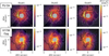 |
Fig. A.3 Same as the bottom panles of Figs. 13 and 14 but for |

Minimum fraction of single-scattering emission to total intensity.
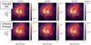 |
Fig. A.4 Same as Fig. 13 but for |

References
- Andrews, S. M., Wilner, D. J., Hughes, A. M., Qi, C., & Dullemond, C. P. 2009, ApJ, 700, 1502 [CrossRef] [Google Scholar]
- Andrews, S. M., Wilner, D. J., Hughes, A. M., Qi, C., & Dullemond, C. P. 2010, ApJ, 723, 1241 [Google Scholar]
- Audard, M., Abraham, P., Dunham, M. M., et al. 2014, Protostars and Planets VI (Tucson: University of Arizona Press), 387 [Google Scholar]
- Bailer-Jones, C. A. L., Rybizki, J., Fouesneau, M., Demleitner, M., & Andrae, R. 2021, VizieR Online Data Catalog: I/352 [Google Scholar]
- Boss, A. P. 2003, ApJ, 599, 577 [NASA ADS] [CrossRef] [Google Scholar]
- Caratti o Garatti, A., Stecklum, B., Garcia Lopez, R., et al. 2017, Nat. Phys., 13, 276 [Google Scholar]
- Cardelli, J. A., Clayton, G. C., & Mathis, J. S. 1989, ApJ, 345, 245 [Google Scholar]
- Chiang, E. I., & Goldreich, P. 1997, ApJ, 490, 368 [Google Scholar]
- Chiang, E. I., & Goldreich, P. 1999, ApJ, 519, 279 [NASA ADS] [CrossRef] [Google Scholar]
- Chiang, E. I., Joung, M. K., Creech-Eakman, M. J., et al. 2001, ApJ, 547, 1077 [NASA ADS] [CrossRef] [Google Scholar]
- Cieza, L. A., Ruíz-Rodríguez, D., Perez, S., et al. 2018, MNRAS, 474, 4347 [CrossRef] [Google Scholar]
- Cotera, A. S., Whitney, B. A., Young, E., et al. 2001, ApJ, 556, 958 [Google Scholar]
- Dong, R., Hashimoto, J., Rafikov, R., et al. 2012a, ApJ, 760, 111 [NASA ADS] [CrossRef] [Google Scholar]
- Dong, R., Rafikov, R., Zhu, Z., et al. 2012b, ApJ, 750, 16r1 [Google Scholar]
- Dong, R., Vorobyov, E., Pavlyuchenkov, Y., Chiang, E., & Liu, H. B. 2016, ApJ, 823, 141 [NASA ADS] [CrossRef] [Google Scholar]
- Draine, B. T., & Lee, H. M. 1984, ApJ, 285, 89 [NASA ADS] [CrossRef] [Google Scholar]
- Dullemond, C. P., Hollenbach, D., Kamp, I., & D’Alessio, P. 2007, Protostars and Planets V, 555 [Google Scholar]
- Elbakyan, V. G., Vorobyov, E. I., Rab, C., et al. 2019, MNRAS, 484, 146 [NASA ADS] [CrossRef] [Google Scholar]
- Fischer, O., Henning, T., & Yorke, H. W. 1994, A&A, 284, 187 [NASA ADS] [Google Scholar]
- Follette, K. B., Grady, C. A., Swearingen, J. R., et al. 2015, ApJ, 798, 132 [CrossRef] [Google Scholar]
- Gramajo, L. V., Rodón, J. A., & Gómez, M. 2014, AJ, 147, 140 [NASA ADS] [CrossRef] [Google Scholar]
- Greenberg, J. M., & Li, A. 1996, A&A, 309, 258 [NASA ADS] [Google Scholar]
- Grosso, N., Alves, J., Wood, K., et al. 2003, ApJ, 586, 296 [Google Scholar]
- Hartmann, L., & Kenyon, S. J. 1996, ARA&A, 34, 207 [NASA ADS] [CrossRef] [Google Scholar]
- Henning, T., & Meeus, G. 2009, arXiv e-prints [arXiv:8911.1818] [Google Scholar]
- Herbig, G. H., Petrov, P. P., & Duemmler, R. 2003, ApJ, 595, 384 [Google Scholar]
- Ilee, J. D., Boley, A. C., Caselli, P., et al. 2011, MNRAS, 417, 2950 [NASA ADS] [CrossRef] [Google Scholar]
- Jäger, C., Mutschke, H., & Henning, T. 1998, A&A, 332, 291 [NASA ADS] [Google Scholar]
- Kim, S., Martin, P. G., & Hendry, P. D. 1994, ApJ, 422, 164 [NASA ADS] [CrossRef] [Google Scholar]
- Kóspál, Á., Abraham, P., Apai, D., et al. 2008, MNRAS, 383, 1015 [CrossRef] [Google Scholar]
- Kóspál, Á., Cruz-Sáenz de Miera, F., White, J. A., et al. 2021, ApJS, 256, 30 [CrossRef] [Google Scholar]
- Laor, A., & Draine, B. T. 1993, ApJ, 402, 441 [NASA ADS] [CrossRef] [Google Scholar]
- Laws, A. S. E., Harries, T. J., Setterholm, B. R., et al. 2020, ApJ, 888, 7 [Google Scholar]
- Liu, H. B., Takami, M., Kudo, T., et al. 2016, Sci. Adv., 2, e1500875 [Google Scholar]
- Long, F., Pinilla, P., Herczeg, G. J., et al. 2018, ApJ, 869, 17 [Google Scholar]
- Lynden-Bell, D., & Pringle, J. E. 1974, MNRAS, 168, 603 [Google Scholar]
- Nayakshin, S. 2010, MNRAS, 408, L36 [NASA ADS] [CrossRef] [Google Scholar]
- Padgett, D. L., Brandner, W., Stapelfeldt, K. R., et al. 1999, AJ, 117, 1490 [CrossRef] [Google Scholar]
- Quanz, S. P., Henning, T., Bouwman, J., et al. 2007, ApJ, 668, 359 [NASA ADS] [CrossRef] [Google Scholar]
- Robitaille, T. P. 2011, A&A, 536, A79 [NASA ADS] [CrossRef] [EDP Sciences] [Google Scholar]
- Robitaille, T. P., Whitney, B. A., Indebetouw, R., Wood, K., & Denzmore, P. 2006, ApJS, 167, 256 [Google Scholar]
- Robitaille, T. P., Whitney, B. A., Indebetouw, R., & Wood, K. 2007, ApJS, 169, 328 [Google Scholar]
- Sandell, G., & Weintraub, D. A. 2001, ApJS, 134, 115 [NASA ADS] [CrossRef] [Google Scholar]
- Shakura, N. I., & Sunyaev, R. A. 1973, A&A, 24, 337 [NASA ADS] [Google Scholar]
- Spitzer, L. 1978, Physical Processes in the Interstellar Medium (Wiley-InterScience) [Google Scholar]
- Stamatellos, D., & Herczeg, G. J. 2015, MNRAS, 449, 3432 [NASA ADS] [CrossRef] [Google Scholar]
- Takami, M., Karr, J. L., Hashimoto, J., et al. 2013, ApJ, 772, 145 [Google Scholar]
- Takami, M., Hasegawa, Y., Muto, T., et al. 2014, ApJ, 795, 71 [Google Scholar]
- Takami, M., Fu, G., Liu, H. B., et al. 2018, ApJ, 864, 20 [Google Scholar]
- Takami, M., Chen, T.-S., Liu, H. B., et al. 2019, ApJ, 884, 146 [NASA ADS] [CrossRef] [Google Scholar]
- Tazaki, R., Tanaka, H., Okuzumi, S., Kataoka, A., & Nomura, H. 2016, ApJ, 823, 70 [NASA ADS] [CrossRef] [Google Scholar]
- Vorobyov, E. I. 2013, A&A, 552, A129 [NASA ADS] [CrossRef] [EDP Sciences] [Google Scholar]
- Vorobyov, E. I., Matsukoba, R., Omukai, K., & Guedel, M. 2020, A&A, 638, A102 [NASA ADS] [CrossRef] [EDP Sciences] [Google Scholar]
- Vorobyov, E. I., Skliarevskii, A. M., Molyarova, T., et al. 2022, A&A, 658, A191 [NASA ADS] [CrossRef] [EDP Sciences] [Google Scholar]
- Watson, A. M., Stapelfeldt, K. R., Wood, K., & Ménard, F. 2007, Protostars and Planets V, 523 [Google Scholar]
- Whitney, B. A., Wood, K., Bjorkman, J. E., & Cohen, M. 2003a, ApJ, 598, 1079 [CrossRef] [Google Scholar]
- Whitney, B. A., Wood, K., Bjorkman, J. E., & Wolff, M. J. 2003b, ApJ, 591, 1049 [Google Scholar]
- Whitney, B. A., Indebetouw, R., Bjorkman, J. E., & Wood, K. 2004, ApJ, 617, 1177 [NASA ADS] [CrossRef] [Google Scholar]
- Whitney, B. A., Robitaille, T. P., Bjorkman, J. E., et al. 2013, ApJS, 207, 30 [Google Scholar]
- Whittet, D. C. B., Gerakines, P. A., Hough, J. H., & Shenoy, S. S. 2001, ApJ, 547, 872 [Google Scholar]
- Wood, K., Wolff, M. J., Bjorkman, J. E., & Whitney, B. 2002, ApJ, 564, 887 [Google Scholar]
- Yen, H.-W., Takakuwa, S., Ohashi, N., et al. 2014, ApJ, 793, 1 [NASA ADS] [CrossRef] [Google Scholar]
- Yen, H.-W., Gu, P.-G., Hirano, N., et al. 2019, ApJ, 880, 69 [NASA ADS] [CrossRef] [Google Scholar]
- Zhu, Z., Hartmann, L., Calvet, N., et al. 2008, ApJ, 684, 1281 [NASA ADS] [CrossRef] [Google Scholar]
- Zhu, Z., Dong, R., Stone, J. M., & Rafikov, R. R. 2015, ApJ, 813, 88 [Google Scholar]
All Tables
Upper limit intensity ratios for the double-scattering emission per single-scattering emission.
Disk parameters for the monochromatic Monte-Carlo radiative transfer simulations.
All Figures
|
Fig. 1 Optical properties for three dust models. From left to right: the opacity per unit gas mass, assuming a gas-to-dust mass ratio of 100 (κext;λ); the scattering albedo ωλ; the forward throwing parameter gλ; and the polarization for the scattering angle of 90°. The gray vertical solid lines indicate three representative wavelengths for our calculations (3.5, 4.8, 12 μm; see text for details). The gray vertical dashed line indicates the wavelength for H band, for which we used imaging polarimetry to model the images for longer wavelengths. The dust opacity κext;λ is shown for the optical to mid-infrared wavelengths, while the remaining parameters for scattered and thermal emission are shown for near- to mid-infrared. The variations of optical properties at λ ~ 3 and ~10 μm are due to water ice and silicate, respectively. |
| In the text | |
|
Fig. 2 Simplified disk geometry with a surface layer and the disk interior. The panels a–d explain the four emission components we discuss in Sect. 3.2.2–3.2.5, respectively. The green arrows indicate scattering of the stellar light at the wavelength of the observations. The blue arrows indicate the stellar light responsible for heating the surface layer and the disk interior. The red arrows indicate thermal emission from the surface layer and the disk interior. In the top panel, β is the radial grazing angle of the disk surface with respect to the incident light from the central illuminating source; δ is the radial inclination angle of the disk surface with respect to the midplane; and θ is the scattering angle. |
| In the text | |
|
Fig. 3
|
| In the text | |
|
Fig. 4 P2(H; θsca) for different dust models. The black solid, dashed and dotted lines at the right side of the panel are the representative constants P2(H) derived using Eq. (11). The gray boxes show the range of the angles used to determine P2(H) (see the text for details). |
| In the text | |
|
Fig. 5 PI distribution in H band, PIobs;H, for FU Ori and V1735 Cyg (Takami et al. 2018), with a pixel scale of 9.5 mas, normalized to the Stokes I flux of the central source. North is up. In each image, the central region is masked as we were not able to make reliable measurement due to the central source being significantly brighter than the extended emission. Features such as spiral arms are labeled (see the text for details). |
| In the text | |
|
Fig. 6 Radiation from the central sources. Top: The spectral energy distributions. The crosses show the observations; the dotted curves show fittings; and the solid curves show those corrected for foreground extinction. Middle: Cumulative fraction of the integrations used in Eqs. (38), (40) and (45). The horizontal axis is the maximum wavelength for integration up to λ=15 μm. Bottom: Same as the middle panels but for the integrations used in Eq. (39). |
| In the text | |
|
Fig. 7 Parameters for disks and envelopes derived from the H band images. From left to right: the aspect ratio for the surface of the extended disk; the radial inclination angle for the surface of the extended disk; the optical thickness of the extended envelope in H band (λ = 1.65 μm) from the central star in the radial direction; the same but for line of sight of the observations. The calculations are made for |
| In the text | |
|
Fig. 8 Histograms for γdisk for the case with a star as the central illuminating source. The vertical axis shows the number of pixels for each bin. The vertical dashed line in each panel shows the representative constant |
| In the text | |
|
Fig. 9 Same as Fig. 7 but with a flat compact disk as the central illuminating source and the ‘Dust3’ model. The white dotted contours in the left two panels indicate the disk surface aspect ratio zdisk/r = 0.5 and the radial inclination of the disk surface δ = 30°, respectively, for the extended disk. The blue and black contours in the right two panels indicate the optical thicknesses τ = 0.35 and 0.7, respectively, in the extended envelope. The gray circle in each panel shows the area where we were not able to execute reliable calculations because of the bright central source in the PI image. The other gray areas indicate the regions where we have not been above to execute self-consistent calculations (see the text). |
| In the text | |
|
Fig. 10 Same as Fig. 8 but with a flat compact disk as the central illuminating source, and with a logarithmic scale for the horizontal axis. |
| In the text | |
|
Fig. 11 Images for the individual emission components. From left to right: the single-scattering component (Ia); thermal emission from the surface layer (Ic) and the disk interior (Id); and the intensity ratio for the thermal emission (Ic+Id) per the single scattering emission for FU Ori at λ =12 μm, assuming that the extended emission is associated with a disk, and |
| In the text | |
|
Fig. 12 Same as Fig. 11 but assuming that the extended emission is associated with an envelope. From left to right: Intensity distributions for the scattered emission |
| In the text | |
|
Fig. 13 Intensities for the single-scattering component for FU Ori at λ = 12 μm, for the cases where the extended emission is due to a disk (top) and an envelope (bottom), and for different dust models. The central illuminating source is assumed to be a flat compact disk. The white dotted contours in the upper panels are for the disk surface aspect ratio zdisk/r = 0.5; the white dotted contours in the lower panels are for the H band optical thickness in the radial direction τr = 0.35 and 0.7; and the black solid contours in the lower panels are for the H band optical thickness along line of sight τl = 0.35 and 0.7. The regions with τr>0.7 and τl>0.7 are hatched in the bottom-right panel. In the top-left panel, the left (east) side of the east arm is masked as the calculations are not self-consistent (see the text). |
| In the text | |
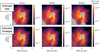 |
Fig. 14 Same as Fig. 13 but for V1735 Cyg. |
| In the text | |
|
Fig. 15 Relative intensities for single scattering emission for various cases. All the values are normalized to that of an extended disk with the ‘Dust1’ model, with a flat compact disk as the illuminating source, and λ = 3.5 μm. The left and right panels are for the case where we assumed the extended emission is associated with a disk and an envelope, respectively, For each panel, we show the intensity ratios for different illuminating sources and dust models. |
| In the text | |
|
Fig. 16 Density distribution used for the monochromatic Monte-Carlo radiative transfer simulations. The green curves show the τ = 1 disk surfaces for κext = 3, 30, and 300 cm2 g−1. |
| In the text | |
|
Fig. 17 Images obtained using monochromatic Monte-Carlo radiative transfer simulations. See text for details. |
| In the text | |
|
Fig. 18 Intensities derived using the new semi-analytic method, divided by those directly derived using monochromatic radiative transfer simulations. As for Fig. 17, the top and bottom panels show images for the face-on view (i=0°–26°) and the intermediate viewing angle (i=37°–46°), respectively. In each panel, the region below the white dashed curve, that are associated with the emission from the outer disk edge, show large variations. These regions were not included in our analysis to verify the calculations (see text for details). |
| In the text | |
|
Fig. 19 Histograms for intensity ratios for Fig. 18 after applying 5 × 5 binning. The dashed vertical panel indicate an intensity ratio of 1. See text for details. |
| In the text | |
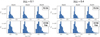 |
Fig. A.1 Same as Fig. 8 but for |
| In the text | |
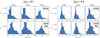 |
Fig. A.2 Same as Fig. 10 but for |
| In the text | |
|
Fig. A.3 Same as the bottom panles of Figs. 13 and 14 but for |
| In the text | |
|
Fig. A.4 Same as Fig. 13 but for |
| In the text | |
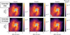 |
Fig. A.5 Same as Fig. A.4 but for V1735 Cyg. |
| In the text | |
Current usage metrics show cumulative count of Article Views (full-text article views including HTML views, PDF and ePub downloads, according to the available data) and Abstracts Views on Vision4Press platform.
Data correspond to usage on the plateform after 2015. The current usage metrics is available 48-96 hours after online publication and is updated daily on week days.
Initial download of the metrics may take a while.