| Issue |
A&A
Volume 676, August 2023
|
|
|---|---|---|
| Article Number | A81 | |
| Number of page(s) | 30 | |
| Section | Stellar atmospheres | |
| DOI | https://doi.org/10.1051/0004-6361/202346018 | |
| Published online | 10 August 2023 | |
Study of a sample of faint Be stars in the exofield of CoRoT
III. Global spectroscopic characterization and astrophysical parameters of the central stars★
1
Sorbonne Université, CNRS, UPMC, UMR7095 Institut d’Astrophysique de Paris,
98bis Bd. Arago,
75014
Paris, France
e-mail: This email address is being protected from spambots. You need JavaScript enabled to view it.
2
GEPI, Observatoire de Paris, PSL Research University, CNRS UMR 8111,
5 place Jules Janssen,
92190
Meudon, France
e-mail: This email address is being protected from spambots. You need JavaScript enabled to view it.
3
European Organization for Astronomical Research in the Southern Hemisphere, Alonso de Cordova
3107,
Vitacura, Santiago de Chile, Chile
4
Royal Observatory of Belgium,
3 Av. Circulaire,
1180
Bruxelles, Belgium
Received:
30
January
2023
Accepted:
12
June
2023
Abstract
Context. The search and interpretation of non-radial pulsations from Be star light curves observed with the CoRoT satellite requires high-quality stellar astrophysical parameters.
Aims. The present work is devoted to the spectroscopic study of a sample of faint Be stars observed by CoRoT in the fourth long run (LRA02).
Methods. The astrophysical parameters were determined from the spectra in the λλ4000–4500 Å wavelength domain observed with the VLT/FLAMES instruments at ESO. Spectra were fitted with models of stellar atmospheres using our GIRFIT package. Spectra obtained in the λλ6400–7200 Å wavelength domain enabled the confirmation or, otherwise, a first identification of Be star candidates.
Results. The apparent parameters (Teff, log g, Vsin i) for a set of 19 B and Be stars were corrected for the effects induced by the rapid rotation. These allowed us to determine: (1) stellar masses that are in agreement with those measured for detached binary systems; (2) spectroscopic distances that agree with the Gaia parallaxes; and (3) centrifugal/gravity equatorial force ratios of ~0.6–0.7, which indicate that our Be stars are subcritical rotators. A study of the Balmer Hα, Hγ and Hδ emission lines produced: (1) extents of the circumstellar disk (CD) emitting regions that agree with the interferometric inferences in other Be stars; (2) R– dependent exponents n(R) = ln[ρ(R)/ρo]/ln(Ro/R) of the CD radial density distributions; and (3) CD base densities ρo similar to those inferred in other recent works.
Conclusions. The Hγ and Hδ emission lines are formed in CD layers close to the central star. These lines produced a different value of the exponent n(R) than assumed for Hα. Further detailed studies of Hγ and Hδ emission lines could reveal the physical properties of regions where the viscous transport of angular momentum to the remaining CD regions is likely to originate from. The subcritical rotation of Be stars suggests that their huge discrete mass-ejections and concomitant non-radial pulsations might have a common origin in stellar envelope regions that become unstable to convection due to rotation. If it is proven that the studied Be stars are products of binary mass transfer phases, the errors induced on the estimated Teff by the presence of stripped sub-dwarf O/B companions are not likely to exceed their present uncertainties.
Key words: stars: early-type / stars: emission-line / Be / stars: fundamental parameters / stars: oscillations
The complete version of Tables D.1 and D.2 are only available at the CDS via anonymous ftp to cdsarc.cds.unistra.fr (130.79.128.5) or via https://cdsarc.cds.unistra.fr/viz-bin/cat/J/A+A/676/A81
© The Authors 2023
 Open Access article, published by EDP Sciences, under the terms of the Creative Commons Attribution License (https://creativecommons.org/licenses/by/4.0), which permits unrestricted use, distribution, and reproduction in any medium, provided the original work is properly cited.
This article is published in open access under the Subscribe to Open model. This email address is being protected from spambots. You need JavaScript enabled to view it. to support open access publication.
1 Introduction
The photometric data obtained by the CoRoT satellite (Weiss et al. 2004; Baglin et al. 2006) concern a wide range of variable objects, including Be stars, which are rapidly, albeit subcritical, rotating objects (Cranmer 2005; Zorec et al. 2016). During their main sequence lifespan, these stars build up a circumstellar disk (hereafter CD), (Jaschek et al. 1981; Collins 1987), whose presence is revealed by line emissions and continuum flux excess, mainly in the visible and infrared spectral domains (Rivinius et al. 2013).
The CoRoT photometric data of Be stars are particularly relevant because they carry signatures of their non-radial pulsation modes. As pulsating objects, Be stars lie in the instability region of the Hertzsprung-Russell (HR) diagram between (or even partially shearing) the instability regions of β Cephei stars and the slowly pulsating-B stars (SPBs, Miglio et al. 2007; Walczak et al. 2015; Saio et al. 2017; Szewczuk & Daszyńska-Daszkiewicz 2017; Burssens et al. 2020). Unlike Be stars, SPBs have often been considered slow rotators. However, long ground-based photometric surveys (e.g., Salmon et al. 2014) and recent four-year data provided by the Kepler mission (Pedersen et al. 2021, and references therein) have enabled the identification of rapid rotators among B-star pulsators (previously considered SPBs), where properties of their internal structure and pulsations might perhaps become an approximation for Be stars (Moravveji et al. 2016).
The analysis of the CoRoT photometric data of Be stars carried out by Huat et al. (2009) and Semaan et al. (2018) revealed complex frequency spectra exhibiting multiple-periodicity and groups of closely separated frequencies, as well as isolated frequencies. This same behavior was also observed in data of Be stars obtained in other space missions: MOST (Walker et al. 2003, 2005a,b), SMEI (Jackson et al. 2004; Goss et al. 2011), KEPLER (Borucki et al. 2010; Kurtz et al. 2015; Pápics et al. 2017), BRITE-Constellation (Weiss et al. 2014; Baade et al. 2016), and TESS (Ricker et al. 2016; Labadie-Bartz et al. 2022).
The groups of closely separated frequencies can be considered as combinations of g-mode pulsations, which cannot be produced by spots in the stellar surface (Kurtz et al. 2015). One of the most important findings in the CoRoT data of HD 49330 (Huat et al. 2009), later also observed in another 7 Be stars analyzed by (Semaan et al. 2018), is the presence of light outbursts accompanied by changes mainly of the photometric power spectrum. They are supposed to be manifestations of discontinuous mass-ejections, similar to those reported by Hubert & Floquet (1998) using HIPPARCOS photometry, as well as in stars of the LMC and SMC observed by the MACHO Cook et al. (1995); Keller et al. (2002) and the OGLE Mennickent et al. (2002), de Wit et al. (2006) surveys. Although these ejections are supposed to provide the required mass to build up a CD as described by the viscous decretion model (VDD), (Lee et al. 1991; Ghoreyshi et al. 2021; Haubois et al. 2012), the mechanisms causing the ejections proper are still heavily debated. On the one hand, from theoretical grounds the combination of prograde g-modes of stellar pulsation could lead to sporadic mass ejections at circumstances when stellar rotation is near critical (Osaki 1986; Kee et al. 2016; Saio et al. 2017). On the other hand, based on spectroscopic studies, Baade et al. (2016) suggested a possible relation between a stellar oscillation called “difference frequency”, which somehow should result from the combination of two other observed close pulsation frequencies, with sporadic mass ejection events. A series of correlations (e.g., Semaan et al. 2018), theoretical predictions of pulsating modes (e.g., Saio 2013), and recent results (e.g., Pápics et al. 2017) confirm that Be stars should be considered as genuine non-radial pulsators.
Two preceding papers by Semaan et al. (2013, 2018) were dedicated to spectroscopic studies and analysis of non-radial pulsation modes in faint Be stars observed in the initial run (IRA01) and the first two long runs (LRC01 and LRA01) of the CoRoT mission. The present work deals with a sample of faint Be stars belonging to the fourth long run (LRA02), whose main objective is to achieve a global spectroscopic characterization for them. The specific aim of the present paper is to determine reliable stellar astrophysical parameters of a new set of faint Be stars. In this work we consider Be stars to behave as single objects.
Although the astrophysical parameters are here determined using spectra obtained in the 4000–4500 Å wavelength domain, spectra in a wavelength region near the Hα line were also obtained in order to confirm the Be star nature of the studied stars. To take full advantage of the obtained spectroscopic data, we also inquire the physical structure of the CD in the studied Be stars. Our approach is based on first principles of radiation transfer that control the formation of Balmer lines. It enables to probe the extents, and the density distribution in the CDs of the studies Be stars.
The present work is organized as follows. Section 2 briefly identifies the sky region of the studied Be stars and specifies the source where the CoRoT data were extracted. Section 3 presents the spectroscopic observations of the program objects. Section 4 gives a short description of the spectral characteristics of the selected Be stars. Section 5 describes the methods used to determine the primary and secondary apparent stellar astrophysical parameters and their treatment for rapid rotation effects. Some correlations between the Balmer line emission intensities and the near-infrared photometric color indices are shown in Sect. 6. A method to describe the physical characteristic of CD of the program stars is detailed in Sect. 7. A short summary of the results obtained is given in Sect. 8.
2 CoRoT observations
The telescope of the CoRoT satellite was pointed to the “anticentre” of the Milky Way to observe the LRA02 field whose coordinates are α = 103°52, δ = −04°38 and Roll = 06°00. Half of the field was dedicated to observation of bright stars devoted to programs of seismology and the other half to observation of faint stars with magnitudes 11 < V < 17 mag to additional programs, such as the search for exoplanets. The upper part of the LRA02 field was very close to the lower part of the IRA01 field, as shown in Deleuil et al. (2016, Fig. III.1.1).
The LRA02 exofield contains stars within coordinates 06h47m30s < α < 06h53m50s and −05°51′30″ < δ < −03°06′30″. In this field, 11448 stars were observed over 112 days from 16 November 2008 to 8 March 2009. CoRoT data, namely, the light curves with several levels of corrections and headers, of all faint stars are available at CDS1.
3 GIRAFFE observations
3.1 Observations and reduction of spectra
A spectroscopic campaign with the VLT/FLAMES instrumentation at ESO2 was undertaken to obtain spectra of the faint Be stars identified in the LRA02 exofield of CoRoT. Observations were conducted in 2010 (November and December) and in 2011 (January). At least three spectra were obtained for each target; one spectrum with 3600 s of exposure time in the MEDUSA MODE at medium resolution, R = 6400, in the LR2 setup (396.4–456.7 nm), hereafter referred to as the “blue spectrum”, and two or three successive spectra with R = 8600 in the LR6 setup (643.8–718.4 nm), hereafter referred to as the “red spectra”, having 780 s of exposure time each. A total of 2209 stars have been observed in 18 fields, of which 2189 ones in two blue and red setups, and 19 stars in only one. We thus dispose spectra for about 19% of the stars that were photometrically observed by CoRoT in the LRA02 exofield. GIRAFFE observations have been conducted at a nearly full moon. Consequently, the stellar spectra are most often polluted by telluric absorption lines and the solar spectrum due to the scattered moonlight. We made the reduction of spectra with the use of the ESO GIRAFFE pipeline in the same way as in Semaan et al. (2013, Paper I) for Be stars studied in the first exofields of CoRoT. Then, we used the IRAF package to separate all the spectra contained in each exposure made in 18 GIRAFFE fields (labeled from a to r). The reduced spectra were calibrated in wavelength, corrected from heliocentric velocity and cleaned for cosmics. For each star, the red spectra were summed up to increase their S/N.
Be star candidates in the LRA02 exofield of CoRoT.
3.2 Setting up the faint Be star sample in the LRA02 exofield of CoRoT
In a first step, we made the selection of emission-line stars by inspecting the Hα line in the red spectrum. We identified about 40 emission-line stars and confirmed two of them: CoRoT 110751872 (TYC 4808-1005-1) and CoRoT 110751876 (EM*AS 136). Moreover, we observed that the Hα line profiles of many fainter B/A stars are often polluted by night sky emission lines (e.g., Hanuschik 2003) which could bring on confusion with regard to the true nature of these objects. We finally selected only 20 Be stars. Other stars are cool or much fainter stars that have noisy spectra polluted by OH lines (Osterbrock et al. 1996) in their Hα line profile.
The selected CoRoT Be star candidates are listed in Table 1. They have been identified in UCAC4 catalog (Fourth U.S. Naval Observatory CCD Astrograph Catalog) and Gaia DR3 catalog (Gaia Collaboration 2023). Information on GIRAFFE spectra and conditions of their exposure times are given in Table A.1. The mean signal-to-noise ratios (S/Ns) range from 40 to 400. The fraction of moonlight that contaminates the spectra is also mentioned.
In a second step, we investigated the blue GIRAFFE spectra of all Be star candidates to identify the photospheric lines in order to determine their spectral type and the corresponding photospheric parameters. Most spectra were obtained for a full moon (see Table A.1). The exposure times in the blue wavelength range are longer than those in the red one. Therefore, the spectra of the faintest stars (15 < V < 17 mag) were more heavily polluted by sky background in the LR2 setup than in the LR6 one. The contamination due to the moonlight was estimated using the processed data of our objects and of their sky environments, which are available in the ESO Science Spectrum archive. We subtracted the moonlight contribution to the flux of each faint star. Thanks to these corrections, we could confirm the B spectral type of all stars in Table 1 (19 stars) and the Be character for 18 of them.
4 Short description of the spectral characteristics of the program Be stars
We present a short description of the spectral characteristics of each Be star candidate in the LRA02 exofield of CoRoT. Several quantities related with Balmer emission lines and shell features are reported. We note that diffuse interstellar bands (DIBs) are often detected in spectra. Most of them are identified at λλ 4232, 4430, 4501, 6614, 6660, 6993, 7060, and 7120 Å (Jenniskens & Desert 1994; Galazutdinov et al. 2000). The spectral region around the Hα line from λ 6500 to 6700 Å of the program stars is shown in Fig. 1.
CoRoT 103000272. Hα shows a faint, double-peaked emission, which is nearly symmetrical (V ≥ R, ∆peaks = 50 km s−1) and centrally superposed on the broad photospheric line profile. No emission is detected in the blue spectrum. We note the presence of very weak metallic lines (Fe II) in the absorption as well as several DIBs.
CoRoT 103032255. Hα shows a strong, single and symmetrical emission line profile. The photospheric red lines He I λλ 6678 and 7065 Å are rather weak. In the blue domain, a very weak emission is present at each side of the core of the photospheric Hγ line profile.
CoRoT 110655185. Hα shows a symmetrical and double-peaked emission line profile (Δpeaks = 110 km s−1) of moderate intensity superimposed on the photospheric line profile; other wavelength ranges in the red spectrum are polluted by telluric lines. A weak emission is present at each side of the core of the photospheric Hγ and Hδ line profiles.
CoRoT 110655384. Hα depicts a very weak, double-peaked emission with V ≥ R and Δpeaks = 290 km s−1 superimposed on the broad photospheric line profile. Weak nebular lines (sky lines) are visible on each Hα side. No emission is detected in blue Balmer lines.
CoRoT 110655437. from its CoRoT light curve, this faint object is known as an eclipsing binary whose period is 3.96685 d (Klagyivik et al. 2017). In the red spectrum, Hα displays a complex line profile with an asymmetric double-peaked emission (V ≫ R, Δpeaks = 367 km s−1) disturbed by two narrow absorptions or shell features, the first one at RV = +155 km s−1, the second at RV = −540 km s−1. He I λ 6678 and 7065 show a double-like structure with a sharp absorption component located at the center of a broad one. Weak nebular lines are present on each side of Hα. It is difficult to search signatures of a binary component in the blue spectrum, which is noisy and has a lower spectral resolution than the red one. Other comments on this object are presented in Sect. 8.2.
CoRoT 110662847. Hα displays a symmetrical, double-peaked emission (Δpeaks = 210 km s−1) superimposed on the photospheric line profile. Red He I lines λλ 6678 and 7065 are conspicuous. No emission is detected in the blue lines.
CoRoT 110663174. Hα shows a nearly symmetrical, double-peaked emission line profile (V ≥ R, Δpeaks = 120 km s−1) of moderate intensity superposed on the photospheric line profile. The blue spectrum of this faint star is very noisy and disturbed by the presence of the full moon in the sky at the epoch of the observation. After correction of this spectrum from sky lines contribution, the core of the photospheric Hγ line profile is disturbed by emission.
CoRoT 110663880. Hα displays a strong emission line profile with a complex, possibly triple structure in its core. The blue spectrum of this faint star is very noisy and strongly affected by the presence of the full moon in the sky at the epoch of the observation. After correction of this spectrum from sky lines contribution, the core of the photospheric Hγ and Hδ line profiles appeared to be disturbed by a double weak emission, itself disturbed by a central shell feature.
CoRoT 110672515. Hα displays a symmetrical, double-peaked emission (Δpeaks = 225 km s−1) with a deep H shell feature (RV = +34 km s−1). Red He I lines are conspicuous; we also note the presence of a metallic shell, mainly of Fe II lines, which depict a weak, double emission on each side of an absorption feature. Hγ and Hδ line profiles are affected by emission on each side of their photospheric core. A shell is also present (H and probably metals) in the blue domain.
CoRoT 110681176. Hα shows a very weak emission, which is nearly symmetrical (V ≤ R, Δpeaks = 295 km s−1) in the core of the photometric line profile. Blue and red He I lines are weak. No emission is observed in the blue Balmer lines.
CoRoT 110688151. Among the Be stars of the sample, this one displays a significant contamination of its spectra due to lines of circumstellar origin. Hα depicts a strong, closely double-peaked emission which is nearly symmetrical (V ≤ R, Δpeaks = 120 km s−1). Red He I lines are conspicuous. In the blue domain, the photospheric Hγ and Hδ line profiles are disturbed in their core by a double-peaked emission. Moreover, the strongest Fe II lines of multiplets 27, 28, 37, 38 in the blue spectrum, and of multiplets 40 and 74 in the red one are present in emission with a double structure. Metallic shell lines highly pollute the blue He I and Mg II lines commonly used to determine stellar astrophysical parameters.
CoRoT 110747131. Hα depicts a weak, closely doubled-peaked emission, which is nearly symmetrical (V ≥ R; Δpeaks = 70 km s−1), in the core of the photospheric line profile. No emission is detected in blue lines.
CoRoT 110751872. Hα shows a symmetrical, closely double-peaked emission of moderate intensity (Δpeaks = 100 km s−1) superimposed on the photospheric profile. Red He I lines are conspicuous. No emission is detected in blue lines.
CoRoT 110751876. This star displays lines formed in the circumstellar medium that contaminate its spectra. Hα shows a rather strong, closely double-peaked emission line (Δpeaks = 140 km s−1), which is symmetrical. In the blue domain, Balmer lines are affected by emission on each side of their photospheric core. Blue He I absorption lines are deep and strong. As in CoRoT 110688151, the stronger lines of the main Fe II multiplets are present with a double emission profile in spectra, which makes particularly difficult the fitting of blue He I and Mg II lines.
CoRoT 110752156. Hα shows a very weak photospheric line profile disturbed on each side by a double-peaked emission (V ≤ R; Δpeaks = 525 km s−1). Moreover, this complex line presents a deep and sharp core in absorption (H shell, RV = +35 km s−1). Red He I lines are conspicuous, He I 6678 depicts a double structure that could be explained as due to binarity, DIP or other facts. The blue spectrum of this faint star is strongly affected by the presence of the full moon in the sky at the epoch of the observation. After correction from sky lines contribution, this spectrum remains noisy, however He I lines are conspicuous as well as a shell H feature in Hγ.
CoRoT 110827583. Hα displays a weak, symmetrical and double-peaked emission (Δpeaks = 170 km s−1) in the core of the broad photospheric line profile. A lot of deep and narrow absorption lines, probably of telluric origin, pollute the red spectrum of this faint object. Moreover, weak nebular lines (OH) are also present on each side of the core of Hα. No emission is detected in the blue domain. After the subtraction of moonlight, the blue spectrum corresponds to a B type star.
CoRoT 300002611. Hα is a weak, symmetrical and double-peaked emission (Δpeaks = 150 km s−1) superimposed to the broad and weak photospheric line. Nebular lines are conspicuous in the vicinity of Hα. Spectra are noisy, the S/N is poor in the bluer part of the blue domain, however weak blue He I lines are detected in this star. Moreover, a weak emission seems to be present at each side of the core of the photospheric Hγ line profile, as well as in Hδ, but with lower intensity.
CoRoT 300002834. Very weak and narrow emission lines (OH) are observed over the wings of the Hα photospheric line; nebular lines [S II] 6717 and 6731 seem also to be present. The emission component in the Hα core could not have a circumstellar origin. Thus, the object is not considered a Be star. We note that fainter early-type stars in the same GIRAFFE field as well as in some others have similar characteristics in their red spectrum.
CoRoT 300003290. Hα shows a strong, single-peaked emission. Very weak sky lines are observed on each side of the line. The photospheric Hγ line is disturbed by a weak, narrow and single-peaked emission in its core. The same is observed in Hδ, but to a lesser degree. As the star is faint, and consequently the blue spectrum is rather noisy, it is difficult to identify whether circumstellar Fe II lines are present or not.
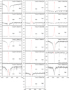 |
Fig. 1 Spectra in the Hα (λ6562 Å) line region of the studied Be stars. This figure also indicates the positions of the He I 6678 line and the diffuse interstellar absorption band at λ6614 Å. The Hα emission component of circumstellar origin is marked in red. The small infilling emission in CoRoT 300002834 is probably not of circumstellar origin. |
5 Astrophysical parameters
The astrophysical parameters derived here are meant to help to estimate the masses, ages, and radii of the program stars. They will enable calculations of rotational frequencies to test the pulsation-instability properties of stars and compare them to theoretical predictions. The determination of the astrophysical parameters implies several steps.
First, a correction from the “veiling” effect of spectra displaying emission lines is needed, which is induced by the disk. Then, the veiling-corrected spectral energy distribution (SED) allows us to access to the “apparent” stellar astrophysical parameters. The apparent parameters are those of classical planeparallel models of stellar atmospheres that correctly represent the spectral characteristics of the studied spectral wavelength region. In our case, this corresponds to the λλ4000–4500 Å interval, emitted by the observed stellar hemisphere, which is deformed by the rapid stellar rotation and has non-uniform surface distributions of gravity and effective temperature. Finally, using models of stellar atmospheres that account for the effects due to rapid rotation, mostly stellar geometrical deformation and gravity darkening (GD), the apparent astrophysical parameters are translated into parent non-rotating counterpart astrophysical parameters (pnrc), which are ultimately used to determine the stellar mass and its age. In this step, we also derive the Vsin i parameter corrected for the GD effect, known as Stoeckley’s underestimation. AA avoids bulleted lists in the man text.
5.1 The veiling effect
The observed continuum energy distribution of Be stars corresponds to the stellar energy emitted by the central stars, modified by the presence of the CD. According to these cases, the positive or negative flux excess produced by the circumstellar environment can represent a significant fraction of the total flux in the visible spectral domain. The apparent residual intensities of spectral lines are meant to be genuine photospheric components that are usually analyzed to infer the astrophysical stellar parameters; thus, they may not only be affected by emission and absorption components produced in the CD, but also can be over- or under-normalized by the continuum energy distribution modified by the flux excess of circumstellar origin. These perturbations have been known from the Fifties, and are called the “veiling effect” (de Jager & Neven 1959; Hawkins 1961). Since then, this effect has been widely studied in the framework of T Tauri stars (Basri & Batalha 1990), but also for Be stars (see, e.g., Hubert-Delplace et al. 1982; Ballereau et al. 1995; Semaan et al. 2013). In order to avoid complex calculations of radiation transfer effects in circumstellar media, which in Be stars are still poorly mastered, we propose taking into account the veiling effect using heuristic expressions that describe the relation between line spectrum Fobs(λ) and the continuum spectrum  emitted by the star+disk system, with F*(λ) and
  attributed to the stellar photosphere. The expression used in this work to carry out the correction of spectra by the veiling effect was discussed in Semaan et al. (2013). Some details regarding this correction and the values of the corresponding veiling factors are given in Appendix B.
5.2 Apparent astrophysical parameters
To derive the apparent astrophysical parameters, plane-parallel model atmospheres were computed for effective temperatures ranging from Teff = 8000–55 000 K and gravities log g = 2.5 to 4.5 dex. We computed the temperature structure of the atmospheres with the ATLAS9 FORTRAN program (Kurucz 1993; Castelli et al. 1997). For effective temperatures of 15 000 K ≤ Teff ≤ 27 000 K, the non-LTE level populations were calculated for the considered atoms using TLUSTY (Hubeny & Lanz 1995) by keeping the temperature and density distributions fixed. We adopted the solar chemical abundances given by Grevesse & Sauval (1998). For model atmospheres with effective temperatures lower than Teff = 15 000 K, full LTE was assumed, while those having Teff > 27 500 K are models from the OSTAR2002 non-LTE grid (Lanz & Hubeny 2003). The grid of fluxes we use during the fitting procedure was built with SYNSPEC. Other computing details of models are given in Frémat et al. (2005, 2006).
The apparent effective temperature and surface gravity are based on the fit of spectral regions not affected by the CE emission/absorption, which encompass wings of hydrogen lines as well as those of helium, carbon, oxygen, silicon, and Mg II lines in the spectral domain from 4000 to 4500 Å. The normalized spectra of the studied stars, Φ*(λ), namely, those corrected for the veiling effect with Eq. (B.1), are Doppler-shifted according to the radial velocity. The fit of the veiling-corrected spectra is carried out by comparing them with a grid of synthetic spectra using the robust least squares method employed in the MINUIT minimization package developed at CERN. This package was transcribed into a FORTRAN language and is named GIRFIT (Frémat et al. 2006). The synthetic spectra were convoluted with a Gaussian function for the required instrumental resolution.
In the most general form, the fitting procedure of spectra with MINUIT considers as an unknown the parametric set (Teff, log g, V sin i, VZ), where VZ is the radial velocity not corrected for the Earth movement around the Sun. The fitting procedure is controlled with the χ2 test computed over zones in the 4000–4500 Å wavelength range where the line circumstellar emissions and shell absorptions and the diffuse interstellar absorption bands are carefully avoided. For three studied stars (stars Nos. 4, 13, and 14) we determined the V sin i using the Fourier transform (FT) method, which was then considered as a fixed quantity. The FT method was applied to the lines He I 4026 and 4472 and Mg II 4481 Å. These objects are the only ones in our sample for which the FT V sin i parameters issued from the three spectral lines are: on the one hand, mutually consistent within the average GIRFIT uncertainty and, on the other hand, consistent with the value obtained with the GIRFIT fitting method.
We note that in spite of the robust character of the MINUIT algorithm, fits of equal quality according to the χ2 test with slightly different values of the set (Teff, log g, V sin i) can be obtained; that is to say: the noise introduces degeneracies in the combination of different parameters, in particular, between log g and V sin i. This phenomenon is worth to be considered in some detail since MV and log L/L⊙ rely sensitively on the value of log g, mainly in late B spectral types. We then introduced a refining protocol to determine the astrophysical parameters that is detailed in the following section.
5.3 Refined astrophysical parameters
In the refining operation of astrophysical parameters, we used the following BCD (Barbier-Chalonge-Divan) calibrations: MV = MV(λ1, D), (Zorec & Briot 1991), Teff = Teff(λ1, D), (Zorec et al. 2009), and log g = log g(λ1, D), (Zorec 1986). To this panoply of relations, we added the expression for the color excesses E(B – V) = [(B – V)obs – (B – V)*], where the intrinsic color index (B – V)* is a function of (Teff, log g). These come from the synthetic UBV colors updated by Castelli F. in 2011 of the model atmospheres published in Castelli & Kurucz (2003). We employed the photometric quantities Vobs and (B – V)obs derived from the (G, BP, RP) magnitudes of the Gaia photometric system (Riello et al. 2021), which represent a uniform photometric data base for our program stars. This uniformity is less obvious among the UBV photometric data proper.
We assumed that the corrections ΔTeff and Δ log g meant to be applied to the first determination of (Teff, log g) can be obtained from the deviations ΔMV and ΔE(B – V) that best approach the condition lim(Δd/d) → 0 derived from Pogson’s formula (Pogson 1856):
![Mathematical equation: ${{{\rm{\Delta }}d} \mathord{\left/ {\vphantom {{{\rm{\Delta }}d} d}} \right. \kern-\nulldelimiterspace} d} = 0.46\left[ {{\rm{\Delta }}{M_{\rm{V}}} + {R_{\rm{V}}}{\rm{\Delta }}E\left( {B - V} \right)} \right].$](/articles/aa/full_html/2023/08/aa46018-23/aa46018-23-eq3.png) (1)
(1)
In Eq. (1), d is the stellar distance and RV = AV/E(B – V) = 3.1 because no other values of RV toward the direction of our program stars are known. In this treatment, the color excess E(B – V)T = (B – V)obs – (B – V)(Teff, log g) has two components:
 (2)
(2)
where E(B – V)ISM is the interstellar extinction proper and E(B – V)CD corresponds to the reddening produced on the Paschen continuum by the CD. We estimated E(B – V)CD with the empirical relation given as a function of the equivalent width Wα of the Hα line emission component used in Gkouvelis et al. (2016), which is based on previous determinations by Raddi et al. (2013) and Dachs et al. (1988). Because the magnitude excess ΔVCD in the V magnitude due to the CD, the reddening E(B – V)CD does not conform to the law RV = AV/E(B – V) = 3.1 that is otherwise valid for the interstellar medium, we must dissociate the circumstellar reddening from the interstellar one and apply it directly to Vobs. While E(B – V)ISM was estimated using Eq. (2) and the noted relation between E(B – V)CD and Wα, the magnitude excess ΔVCD was obtained from Eq. (8) in Zorec & Briot (1991).
When dealing with Eq. (1), knowledge of d is never required. We simply parameterized the ratio Δd/d from −0.5 to +0.5, and for each Δd/d we tested a series of values ΔMV and ΔE(B – V), which (via the above BCD calibrations) enable us to calculate the corrections ΔTeff and Δ log g. The chosen fit with GIRFIT then corresponds to the smallest possible value found of |Δd/d| that leads to the best χ2 test. From this fit, we get not only the apparent astrophysical parameters (Teff, log g, V sin i), but also MV and E(B – V)ISM. In most cases, it is |(Δd/d)| ≲ 0.05.
Specifically, BCD calibrations of astrophysical parameters are displayed in tabular forms and can be reverted to: MV = MV(Teff, log g) and E = E(B – V)(Teff, log g), from which the required relations readily follow:
 (3)
(3)
needed to derive ΔTeff and Δ log g from ΔMV and ΔE(B – V). The best fits of the observed spectra previously corrected for the veiling effect obtained with GIRFIT, subject to the noted iteration procedure, are shown in Appendices as Figs. C.1–C.4. The apparent astrophysical parameters derived are given in Table 2. We refer to them as the “primary apparent astrophysical parameters”.
Due to the noted subtleties that have to be taken into account to calculate the spectroscopic distances of Be stars, it is worth specifying Pogson’s formula, as it is used in the present work:
 (4)
(4)
Once the final couple (Teff, log g) was adopted, we calculated the uncertainties associated to the estimated distances marked in tables of results, which depend only on the measurement errors of Vobs and (B – V)obs, E(B – B)ISM and Iα. Each of these parameters is represented as X + ϵX, where the error ϵX is simulated through a Monte Carlo procedure. The errors ϵX are assumed having a normal distribution characterized by the respective standard dispersion σX reported in our tables. The reported values of dspect in Table 3 are the averages 〈dspect〉 of 104 estimates, and σd represents their standard deviation. The same procedure was adopted also for 〈dGaia〉 = 〈1/(π + ϵπ)〉, where ϵπ is considered to have a normal distribution with the standard deviation published for each Gaia DR3 parallax π (Gaia Collaboration 2016, 2021; Lindegren et al. 2021). The errors associated to MV in Table 3 are also due to Vobs, (B – V)obs, E(B – B)ISM and Iα.
Primary and secondary apparent astrophysical parameters.
5.4 Secondary apparent astrophysical parameters
We use the term “secondary apparent astrophysical parameters” to apply to all those that tightly depend on the “primary apparent astrophysical parameters” and were not obtained from the fitting operation of spectra. Some of them also rely on models of stellar evolution. These are: the BCD parameters (λ1, D), the bolometric luminosity, log L/L⊙, the stellar mass, M/M⊙, equatorial radius, R/R⊙, the equatorial linear critical velocity, Vc, and the fractional stellar age, t/tMS (t is the age and tMS is the time that a non rotating star spends in the main sequence evolutionary phase).
The BCD quantities (λ1, D) are determined from the adopted (Teff, log g) parameters, which in turn lead to the BCD spectral classification of the studied Be stars (Zorec & Briot 1991; Zorec et al. 2009). This set of secondary apparent parameters is given in Table 3.
Adopting the bolometric correction BC(Teff) by Flower (1996), to avoid possible conflicts with the zero point of bolometric corrections, we determined the bolometric “apparent” absolute magnitude Mbol following the prescription from Torres (2010):
![Mathematical equation: ${M_{{\rm{bol}}}} = M_{{\rm{bol}}}^ \odot + \left[ {{M_{\rm{V}}} - M_{\rm{V}}^ \odot } \right] + \left[ {{\rm{BC}}\left( {{T_{{\rm{eff}}}}} \right) - {\rm{BC}}\left( \odot \right)} \right].$](/articles/aa/full_html/2023/08/aa46018-23/aa46018-23-eq17.png) (5)
(5)
From this, we can derive the bolometric luminosity, log L/L⊙. Once log L/L⊙ and  are determined, we estimate the stellar radius R/R⊙. Finally, by interpolating in the grids of stellar evolutionary models without rotation given by Georgy et al. (2013) for solar metallicity Z = 0.014, we obtain the stellar masses M/M⊙ and its fractional ages t/tMS. All these secondary apparent astrophysical parameters are reported in Table 2 with their uncertainties.
To complete the presentation of the program objects, we show their HR diagram in Fig. 2, where we have included the instability zones calculated by Walczak et al. (2015) for non rotating objects using the OPLIB new Los Alamos opacities. Similar calculations can be found in Miglio et al. (2007), Burssens et al. (2020) for other opacities, and rotating stars in Saio et al. (2017) and Szewczuk & Daszyńska-Daszkiewicz (2017), where the widening of the instability regions due to stellar rotation can be seen.
Indirect apparent quantities, interstellar reddening, and distances.
5.5 Astrophysical parameters corrected for effects carried by the rapid rotation
We consider that the stars are rigid rotators characterized by a uniform surface rate of angular velocity ratio Ω/Ωc, where Ωc is the surface angular velocity at critical rotation. The apparent astrophysical parameters obtained in Sect. 5.2 can then be given according to the following formal expression:
 (6)
(6)
where P stands for parameters as effective temperature, Teff, surface gravity, g, bolometric luminosity, L, and projected rotational velocity, V sin i. On the left-hand side of Eq. (6), these quantities are considered “apparent”, that is, they are issued from models of stellar atmospheres and evolution without rotation that fit the observed spectral domain. On the right side of Eq. (6), the parameters P correspond to the parent-non-rotating-counterparts (pnrc; Frémat et al. 2005), which are multiplied by functions that represent the effects carried by a rapid rotation in an object of actual mass, M, and age, t, whose surface angular velocity is Ω and its rotational axis is seen according to an aspect angle, i.
The functions FP(M, t, Ω, i) in Eq. (6) were calculated with FASTROT (Frémat et al. 2005) as follows. For a series of stellar masses, ages, and rotational rates, we calculated 2D models of stellar structure assuming rigid rotation over the whole star (Zorec et al. 2011; Zorec & Royer 2012). The geometrical deformations of stars induced by the rapid rotation produce a surface gravity that depends on the latitude and a non uniform distribution of the effective temperature, which is calculated by the gravity darkening formula given by Espinosa Lara & Rieutord (2011). Using local plane-parallel model atmospheres, we recomposed the apparent stellar spectra in the λλ4000–14500 Å wavelength region for objects of several masses, ages, angular velocity rates Ω/Ωc, and inclination angles, i. The system of equations in Eq. (6) is given in a tabular form whose solutions for the unknown quantities (M, t, Ω/Ωc, i) are obtained by iteration. Since only Teff, log g and V sin i as entry apparent parameters can be considered independent, we solved these equations for a series of imposed values of Ω/Ωc. Due to gravitational darkening, the observed (apparent) V sin i are underestimated (Stoeckley 1968; Townsend et al. 2004; Frémat et al. 2005). The amount of this underestimation is automatically taken into account in the solution of Eq. (6). The evolutionary tracks of rotating stars used were calculated by Georgy et al. (2013) and are given in terms of effective temperatures and bolometric luminosity averaged over the surface of the geometrically deformed rotating objects. This imposes that at each iteration step, the corresponding averaged quantities over the stellar surface are calculated from the running pnrc parameters. Moreover, at each iteration step we need to determine the rotational velocity of stars in the ZAMS to identify the right evolutionary track needed to interpolate the stellar mass and age at the running stellar age, which is consistent with the imposed rotational rates Ω/Ωc. Once a cycle of iterations is over, we calculate the rotational frequency, vr, given by:
![Mathematical equation: $\matrix{ {{v_{\rm{r}}} = 0.02\,\left[ {{{{V_{{\rm{eq}}}}\left( {{{\rm{\Omega }} \mathord{\left/ {\vphantom {{\rm{\Omega }} {{{\rm{\Omega }}_{\rm{c}}},M,t}}} \right. \kern-\nulldelimiterspace} {{{\rm{\Omega }}_{\rm{c}}},M,t}}} \right)} \over {{R_{{\rm{eq}}}}\left( {{{\rm{\Omega }} \mathord{\left/ {\vphantom {{\rm{\Omega }} {{{\rm{\Omega }}_{\rm{c}}},M,t}}} \right. \kern-\nulldelimiterspace} {{{\rm{\Omega }}_{\rm{c}}},M,t}}} \right)}}} \right]} & {{{{\rm{cycles}}} \mathord{\left/ {\vphantom {{{\rm{cycles}}} {{\rm{day}}}}} \right. \kern-\nulldelimiterspace} {{\rm{day}}}}} \cr } , $](/articles/aa/full_html/2023/08/aa46018-23/aa46018-23-eq20.png) (7)
(7)
where Veq is the equatorial linear velocity given in km s−1 and Req is the equatorial radius in solar units of the star distorted by its rotation.
Each entry parameter in Eq. (6) is considered with its uncertainty assumed having a normal (Gaussian) distribution. We produced 104 Monte Carlo trials of all entry parameters and each time we sought a new solution for the system using Eq. (6). Sometimes, the set of entry parameters ( ,
,  ,
,  ,
,  ) may not correspond to realistic objects. In such cases, the functions FP(M, t, Ω, i) cannot produce a reliable solution and the trial is considered as having no solution. Although the uncertainties of the entry parameters are assumed to have normal distributions, the distributions of the solution quantities do not always have normal distributions. So, the averages of parameters with non symmetrical distribution do not coincide with the mode of the distribution (mode = parameter corresponding to the maximum of the distribution). In order to illustrate the obtained differences in the estimated parameters, we produced two tables of results: one of them gives the average values of solutions with their classical standard 1σ deviations, while the other is for modes, where the “sigmas” correspond to the uncertainties related to the identification of the modes. Similar solutions to the system Eq. (6) have been previously done in Floquet et al. (2000), Neiner et al. (2003), Frémat et al. (2005), Zorec et al. (2005), Zorec et al. (2016), Vinicius et al. (2006), Martayan et al. (2006, 2007), Semaan et al. (2013). In Appendix D, Tables D.1 and D.2 give the averages and modes of distributions of astrophysical parameters and rotational frequencies corrected for rotational effects assuming Ω/Ωc = 0.95, respectively. These tables give: the pnrc effective temperature, Teff, log g, true V sin i, pnrc bolometric luminosity in solar units, log L/L⊙, mass M/M⊙, critical linear equatorial velocity, Vc, estimated inclination angle, i, true fractional age, t/tMS, the true stellar age, t, and the rotational frequency, vr, in cycles/day. All these quantities are given with their respective 1σ dispersion calculated from the obtained distribution of solutions. Similar solutions obtained for imposed values Ω/Ωc = 0.8,0.9,0.999, and 1.0 are given in Tables D.1 and D.2, respectively, available at the CDS.
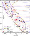 |
Fig. 2 HR diagram of the studied stars. Evolutionary tracks are from Georgy et al. (2013) for Ω/Ωc = 0.0 (blue) and for rotation rates at the ZAMS Ω/Ωc = 0.95 (red). Blue points: stars with their apparent parameters; red points: Stars with their pnrc parameters obtained for Ω/Ωc = 0.95. Instability strips of β Ceph- (-) and SPB-type (-) pulsators adapted from Walczak et al. (2015) for OPLIB opacities and metallicity of Z = 0.015. |
6 Some empirical relations concerning the CD in the studied Be stars
The close relation between the spectroscopic distances and those measured by Gaia, provide us with some confidence on the reliability of the inferred astrophysical parameters. We can then try to benefit from some information on the properties of CDs of the studied stars, drawn from the emission in spectral lines. Thanks to the derived astrophysical parameters, good estimates of the neat emission line profiles and of the amount of emission filling up the photospheric component of the here observed Balmer lines Hα, Hγ, and Hδ can be obtained, at least when it is possible according to the S/N of the spectra.
6.1 Total emission in the observed Balmer lines
In cases when the emission in a line clearly exceeds the continuum over its entire wavelength range, we can simply add to this latter the amount of emission that fills up the photospheric absorption component derived from the stellar astrophysical parameters. If this filling up is partial, here the apparent photospheric absorption profile underlying the emission is called the pseudo-photospheric absorption. We estimated the pseudo-photospheric absorption and add to this last the difference between the pseudo-photospheric and the photo-spheric proper absorption line profile. The pseudo-photospheric (pph) absorption line profile is easily fitted using the relation ψ(λ) = exp {−1/[a + b × (λ − λo)c]} introduced by Ballereau et al. (1995), Chauville et al. (2001), where the constants a, b, and c are determined using only three points in the line profile. In Fig. 3, the red lines show the total Hα line-emission components reduced to the continuum intensity level Iλ/Ic = 1 (violet dotted line). Thus, the total emission profile (red line) makes up the observed profile proper, to which the residual intensity between the photospheric profile and the pseudo-photospheric absorption profile has been added. The blue dashed lines correspond to the photospheric absorption line profile broadened according to the measured V sin i parameter. The green dashed lines are the pseudo-photospheric absorption line profiles. The equivalent width of the total Hα emission corresponds then to the area below the red profile and the Iλ/Ic = 1 line, that is,  . In Table 4, we give the equivalent widths WHα,
  ,
,  , and
, and  .
.
The line emission profiles in the Hγ and Hδ lines are determined through the residual intensities between the emission proper and the photospheric line profile. We also assume that the emission in these lines is weak enough to take the pseudo-photospheric profile as the genuine photospheric absorption. In Fig. 4, we reproduce the emission line profiles in Hγ and Hδ lines. Some emission in these lines can also be present in other stars, but they are too noisy to carried out a clear extraction. We attempted to determine the equivalent width for all detectable emissions; they are given in Tables 4 and B.1 and were previously used in Sect. 5.1 to calculate the veiling factor.
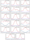 |
Fig. 3 Smoothed Hα line-emission components (red profiles). The emission residual intensities are relative to the photospheric line calculated according to the astrophysical parameters (Teff, log g, V sin i) of each object. The figure shows the photospheric component broadened by rotation (blue profiles). It includes the empirical pseudo-photospheric component (green profiles, see Sect. 6.1) in cases of partial emission feeling up of the absorption photospheric line. For the stars 103000272, 110681176, 110747131, and 110827583, the fit of the observed pseudo-photospheric absorption component closely reproduces the actual photospheric line. |
6.2 Other measurements on the emission line profiles
An estimate of the total extent of the CD line emission formation region is frequently done using a relation which assumes that the disk is optically thin and that it has a rotation law that is dependent of the distance R/Ro (Ro is radius of the base of the disk) from the central star (Huang 1972). Following the reasoning in Arcos et al. (2017) we can write Huang’s radius as
 (8)
(8)
where Δp is the distance in km s−1 between the emission peaks, and j = 1/2 if the rotation is Keplerian or j = 1 if the disk conserves the angular momentum. The factor of 2.7 in Eq. (8) differs from that used in Arcos et al. (2017), because stellar deformations were calculated following Frémat et al. (2005) for Ω/Ωc = 0.88. In Table 5, we give the measured emission peak separations and the disks extents R/Ro determined assuming Keplerian rotation (j = 0.5). To avoid confusion, we note that Huang’s radius (R/Ro)H in Table 5 is calculated with Δp, while (R/Ro)hm represents a kind of Huang’s CD extent determined with the full-widths-at-half-maximum (FWHM), Δhm, of the respective Balmer emission lines. The radius (R/Ro)H is meant to represent the extent of the entire region in the CD where the emission is raised, if the CD is optically thin, while (R/Ro)hm represents just a part of this line-forming region. The width of the base of emission line should in principle correspond to (R/Ro)base = 1. However, the wings of emission lines are affected by other broadening mechanisms apart from rotation, so that the relation in Eq. (8) cannot identify well defined distances in the CD when using the FWHM or the width at the base of emission lines. Relations with the V sin i of the peak separations Δp and line widths at half intensity Δhm of the emission components in the Hα, Hγ and Hδ lines are shown in Fig. 5.
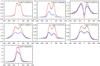 |
Fig. 4 Smoothed Hγ (red) and Hδ (blues) line-emission components. The emission residual intensities are relative to each photospheric line. Emissions in these Balmer lines are seen also in some other stars, but they are too noisy and not exploitable. |
Equivalent widths and normalized fluxes of the emission components in the Hα and Hδ lines.
6.3 Near-IR circumstellar color excess and the Balmer line emissions
To complete the presentation of observational characteristics of the program Be stars, we include in this section a short discussion of their near-IR photometric data. These allow us, on the one hand, to situate them in the color-color diagram and show they do not belong to the B[e] class of stars known as Herbig HAe/Be, and on the other hand, to obtain some relations commonly used to present the Be phenomenon (Ashok et al. 1984; Dachs et al. 1988; Hanuschik 1989; Kastner & Mazzali 1989). However, it is not in the scope of the present work to extract information on the CDs from the photometric data.
Be stars present a thermal IR flux excess mainly due to bound-free, free-free transitions, and electron scattered radiation in their CD. To characterize the energy distribution in the visible domain, we could use the (B – V) color index from the UBV Johnson-Cousins photometric system derived from the (G, GBP, GRP) Gaia photometry using the published transformation relations into the UBV photometric system (Riello et al. 2021) in the way that has widely been studied by Moujtahid et al. (1998, 1999). However, this color index is heavily marred by the interstellar reddening so that the genuine color excess due to the CD is marred by the uncertainties of the E(B – V)ISM color excess determinations. We then used the near-IR photometry in the J, H, and K bands to try to characterize the color excess produced by the Be star CD. To this end, the 2MASS photometry (Cutri et al. 2003) was used.
The observed (J – H)obs and (H – J)obs colors were corrected from interstellar extinction using the relations between the color excesses E(V – J) = 2.23 E(B – V), E(V – H) = 2.55 E(B – V), and E(V – K) = 2.76 E(B – V) and the reddening relation, AV = 3.1E(B – V), established by J. S. Mathys (1999, priv. comm.) and published in Cox (2000), Kinman & Castelli (2002). The determination of the color excess E(B – V) was detailed in Sect. 5.4. The JHK dereddened color-color diagram of the studied stars is shown in Fig. 6 (red stars), where we added the model sequences of intrinsic colors for log g = 1.0 to 5.0 dex by Castelli & Kurucz (2003, updated in 2011), and the region occupied by the bluest Herbig HAe/Be stars (Hernández et al. 2005) to show that our program stars were not mistakenly chosen among Herbig HAe/Be objects. The stars numbered 17 and 19 have much larger JHK color uncertainties than the remaining ones, which might explain their extreme blue (H – K)o colors.
The color excesses proper in the IR that characterize the flux excess produced by the CD are defined as
 (9)
(9)
where (J – H)* and (H – K)* are the respective intrinsic colors of stars that underlay the CD. The intrinsic colors are inferred from the synthetic colors indices calculated with LTE models of stellar atmospheres by Castelli & Kurucz (2003), using the apparent (Teff, log g) parameters. Also, (J – H)o and (H – K)o are the observed color indices corrected for the ISM extinction.
Having at our disposal observations in the Ha line as well as, for some stars, also in the Hγ and Hδ reliable line emissions – we can look for a correlation between the flux IR color excess and the intensity of the emission component in the Balmer line emission components. Because the IR flux excess and the Balmer line emissions are produced in rather different regions of the same CD, such correlations can be of interest in attempting to control the consistency of physical inputs meant to describe the structure of Be star disks and their formation mechanisms. Marginally, we note that the sought correlations are marred by uncertainties due mainly to the non-simultaneity of observations carried of the IR colors and of the Balmer lines, as well as of the physical origins. In fact, since the perturbations produced by the CD on the continuum spectrum and on the line emissions are not produced in the same layers, there may be line emission intensities produced rather far from the star (roughly 2 Ro ≲ R ≲ 10 Ro) that correspond to positive or negative flux excesses coming from disk layers near the star, generally R ≲ 2 Ro. In spite of these shortcoming, we can attempt to establish some relations with the data at disposal in the way were previously attempted in Ballereau et al. (1995) between the flux excess ΔV in the magnitude V and the Hγ line emission, which revealed a quite reliable and useful correlation, which is described in Sect 5.1 as a way of correcting the observed spectra from the veiling effect in the λλ4000–4500 Å spectral range.
The emission intensities at Hα, Hγ, and Hδ lines are given by:
![Mathematical equation: ${I_{{\rm{H}}\alpha {\rm{,H}}\gamma ,{\rm{H}}\delta }} = W_{{\rm{H}}\alpha ,{\rm{H}}\gamma ,{\rm{H}}\delta }^{{\rm{em}}} \times \left[ {{{F_{{\rm{H}}\alpha ,{\rm{H}}\gamma ,{\rm{H}}\delta }^{\rm{c}}} \over {F_{{\rm{H}}\alpha {\rm{,H}}\gamma ,{\rm{H}}\delta }^{\rm{c}}\left( {22\,500,4.0} \right)}}} \right],$](/articles/aa/full_html/2023/08/aa46018-23/aa46018-23-eq35.png) (10)
(10)
where  are the equivalent widths of the emission components in the Hα, Hγ, and Hδ lines,
  are the fluxes of the continuum spectrum at the center of the lines, and
  (22 500,4.0) are the normalizing fluxes given by a model with Teff = 22 500 K and log g = 4.0 (roughly a B2V type star). In Table 4, we give the equivalent widths
  of the emission component in the Hα and Hγ lines, and the respective intensities IHα and IHγ. In Fig. 7, we show the trends determined by IHα, IHγ, and IHδ against the color index excess Δ(J – H)CD, which are rather well defined, while the correlations of the line emission intensities with Δ(H – K)CD, not shown here, look much more scattered. In Table 6, we give the observed color indices (J – H)obs and (H – K)obs, the adopted stellar intrinsic colors (J – H)* and (H – K)*, and the color index excess Δ(J – H)CD.
Separation of emission peaks Δp, line emission FWHM, Δhm, and Huang’s radius of the CD according to Δp and Δhm.
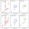 |
Fig. 5 Relations with the V sin i of the peak separations Δp and line widths at half intensity Δhm of the emission components in the Hα (red), Hγ (blue) and Hδ (green) lines. A black circle surrounds the binary star N° 5. |
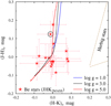 |
Fig. 6 Dereddened JHK color-color diagram of the program Be stars. The JHK magnitudes are from 2MASS. In this diagram are also shown the model sequences of the intrinsic colors corresponding to log g = 1.0, 3.0, and 5.0 dex, and the corner occupied by the bluest Herbig HAe/Be stars. A black circle surrounds the binary star N° 5. |
7 Physical characteristics of CDs derived from the interpretation of the Balmer line emission components
In this section we explore the properties of the CDs derived from the spectroscopic characteristics of the Hα, Hγ, and Hδ emission lines. We produce a simple representation of the CD that may contrast in simplicity with more detailed calculations as those by Carciofi & Bjorkman (2006, 2008), Sigut & Jones (2007), Sigut et al. (2009), McGill et al. (2013), Catanzaro (2013), Kurfürst et al. (2018). The simplifications we use are based on first physical principles and are introduced in as physically consistent a way as possible.
7.1 Assumptions about the geometry and temperature of the CD
To describe the geometrical characteristics of the CD, we use two reference systems centered on the star. In the star system (X, Y, Z), the Z–axis contains the rotation axis, while (X, Y) are in the stellar equatorial plane with X on the back sky plane. The system (x, y, z) has the z–axis directed towards the observer, and x coincides with X. The angle between Z and z is the inclination angle, i, of the star-disk system. The radius vector, R, is measured on the (X, Y) plane. Between Y and R, there is the azimuth angle θ.
We take the CD driven by a quasi-Keplerian speed of rotation VK(R) = V°K(Ro/R)γ/2. We include an expansion (or contraction) velocity parameter Vexp to account for the emission line profile asymmetry. The integration of the hydrostatic equilibrium equation for the circumstellar environment leads to the axisymmetric density profile of the disk given in Kurfürst et al. (2018), of which we adopt the simplified expression valid for Z/R ≪ 1:
![Mathematical equation: $\rho \left( {R,z} \right) = {\rho _o}D\left( R \right)\,{\rm{exp}}\,\left\{ { - {{\left[ {{Z \mathord{\left/ {\vphantom {Z {\sqrt 2 h\left( R \right)}}} \right. \kern-\nulldelimiterspace} {\sqrt 2 h\left( R \right)}}} \right]}^2}} \right\}, $](/articles/aa/full_html/2023/08/aa46018-23/aa46018-23-eq40.png) (11)
(11)
which still describes the main geometrical characteristics of disks and enables easier mathematical handling. In Eq. (11), ρo is the base density of the disk at the stellar equator, D(R) is a function meant to describe the CD density distribution in the equatorial plane, and h(R) = [Vs/VK]R is the Z-scale height of the disk with Vs as the sound speed and VK as its quasi-Keplerian rotation. Explicitly
![Mathematical equation: $\left. {\matrix{ {h\left( R \right) = k{{\left[ {{{\left( {{{{R_o}} \mathord{\left/ {\vphantom {{{R_o}} {{R_ \odot }}}} \right. \kern-\nulldelimiterspace} {{R_ \odot }}}} \right)}^\gamma }{{\left( {{{{T_{{\rm{eff}}}}} \mathord{\left/ {\vphantom {{{T_{{\rm{eff}}}}} {{T_ \odot }}}} \right. \kern-\nulldelimiterspace} {{T_ \odot }}}} \right)} \mathord{\left/ {\vphantom {{\left( {{{{T_{{\rm{eff}}}}} \mathord{\left/ {\vphantom {{{T_{{\rm{eff}}}}} {{T_ \odot }}}} \right. \kern-\nulldelimiterspace} {{T_ \odot }}}} \right)} {\left( {{M \mathord{\left/ {\vphantom {M {{M_ \odot }}}} \right. \kern-\nulldelimiterspace} {{M_ \odot }}}} \right)}}} \right. \kern-\nulldelimiterspace} {\left( {{M \mathord{\left/ {\vphantom {M {{M_ \odot }}}} \right. \kern-\nulldelimiterspace} {{M_ \odot }}}} \right)}}} \right]}^{{1 \mathord{\left/ {\vphantom {1 2}} \right. \kern-\nulldelimiterspace} 2}}}{{\left( {{R \mathord{\left/ {\vphantom {R {{R_o}}}} \right. \kern-\nulldelimiterspace} {{R_o}}}} \right)}^\beta }} \hfill \cr {k\quad \,\,\, = {{\left[ {{{\cal R} \mathord{\left/ {\vphantom {{\cal R} {\left( {\sqrt 2 \mu G} \right)\left( {{{{R_ \odot }T_{{\rm{eff}}}^ \odot } \mathord{\left/ {\vphantom {{{R_ \odot }T_{{\rm{eff}}}^ \odot } {{M_ \odot }}}} \right. \kern-\nulldelimiterspace} {{M_ \odot }}}} \right)}}} \right. \kern-\nulldelimiterspace} {\left( {\sqrt 2 \mu G} \right)\left( {{{{R_ \odot }T_{{\rm{eff}}}^ \odot } \mathord{\left/ {\vphantom {{{R_ \odot }T_{{\rm{eff}}}^ \odot } {{M_ \odot }}}} \right. \kern-\nulldelimiterspace} {{M_ \odot }}}} \right)}}} \right]}^{{1 \mathord{\left/ {\vphantom {1 2}} \right. \kern-\nulldelimiterspace} 2}}}} \hfill \cr } } \right\}, $](/articles/aa/full_html/2023/08/aa46018-23/aa46018-23-eq41.png) (12)
(12)
with ℛ the constant of gases; µ the average molecular weight; gravitational constant G; R⊙,  , and M⊙ are the solar radius, effective temperature, and mass, respectively. In the following, we use γ = 1 to otherwise describe deviations from a strict Keplerian rotation. Whether the temperature of CD follows the geometrical dilution of the stellar bolometric radiation or whether it is isothermal, we take either β = (2 + γ − 1/2)/2 = 1.25 or β = (2 + γ)/2 = 1.5, respectively.
The function D(R) can be specified only if a theory is used to describe the formation and further evolution of the CD, as done in VDD models (Narita et al. 1994; Okazaki 2001; Haubois et al. 2012; Ghoreyshi et al. 2021; Marr et al. 2021). In this work, we assume that the R–dependent density profile of the disk is parameterized as D(R) = (Ro/R)n, where the exponent n is a function of R. The density exponent, n, that is reported currently in the literature, actually represents the global slope of the disk density variation with R. However, from Haubois et al. (2012), it is clear that depending on the evolution phase of the circumstellar disk, n(R) is a strong function of R, mainly in proximity to the star, where emission component in lines such as Hγ and Hδ are formed. Anticipating the possibility that the regions where the emission of Hα and those of Hγ and Hδ do not respond to the same value of the density exponent n, as in Zorec et al. (2007), we adopted the following expression for n(R):
![Mathematical equation: $\matrix{ {n\left( R \right) = \left[ {{{\left( {{n_2} - {n_1}} \right)} \mathord{\left/ {\vphantom {{\left( {{n_2} - {n_1}} \right)} \pi }} \right. \kern-\nulldelimiterspace} \pi }} \right]\,\arctan \,\left\{ {Q \times \,\left[ {\left( {{R \mathord{\left/ {\vphantom {R {{R_o}}}} \right. \kern-\nulldelimiterspace} {{R_o}}}} \right) - \left( {{{{R_D}} \mathord{\left/ {\vphantom {{{R_D}} {{R_o}}}} \right. \kern-\nulldelimiterspace} {{R_o}}}} \right)} \right]} \right\}} \hfill \cr {\,\,\,\,\,\,\,\,\,\,\,\,\,\,\,\,\, + \left( {{1 \mathord{\left/ {\vphantom {1 2}} \right. \kern-\nulldelimiterspace} 2}} \right)\left( {{n_1} + {n_2}} \right),} \hfill \cr } $](/articles/aa/full_html/2023/08/aa46018-23/aa46018-23-eq43.png) (13)
(13)
whose value changes from n(R) = n1 within Ro ≲ R ≲ RD to n(R) = n2 > n1 for R ≳ RD. In Eq. (13), Q ≲ 10 is a constant chosen freely. However, no significant changes are carried on the determination of parameters if we adopt a simple step relation n(R) = n1 at Ro ≤ R ≤ RD and n(R) = n2 for R ≳ RD.
From the theory of VDD (Lee et al. 1991; Okazaki 2001, 2007), we know that in isothermal disks at the steady state, it is n = 3.5 over the entire disk radial extent. The results obtained by Zorec et al. (2007) based on the study of Fe II emission lines in the blue spectral range of Be stars, suggest that n1 ≲ 1.0 for R ≲ RD ~ 3Ro, while studies on the SED in the near- and far-IR of Be stars (Waters 1986; Vieira et al. 2015) suggest n2 ≃ 2.5–3.9 for R ≳ RD. The modeling of the SED in the 3500–10 500 Å wavelength interval of a set of Be stars by Moujtahid (1998) Moujtahid et al. (2000a,b) and Chauville et al. (2001) suggested an average exponent < n >= 1.6 ± 0.2. Granada et al. (2010) used n1 = 0.5 in a study of emissions in the hydrogen Humphry’s series, which form in CD regions near the central star. Studies of the temporal evolution of VDD density distributions under different formation scenarios (Haubois et al. 2012) end up concluding that n varies from 0.5 to 4.5, but sometimes n < 0 in the base of the disk. The function n(R) on the distance from the star, it is sensitive to the kinematic viscous coefficient and depends on the disk decretion history (Haubois et al. 2012; Vieira et al. 2017; Ghoreyshi et al. 2018, 2021; Marr et al. 2021).
In a large series of papers, disk models for Be stars were assumed to be isothermal (Marlborough 1969; Poeckert & Marlborough 1978a,b; Hummel 1994; Catanzaro 2013). More refined discussions on the distribution of the temperature in the CD of Be stars obtained high non-uniform temperature distributions, whose global behavior depends on the physical inputs and assumptions made in the models. Millar & Marlborough (1998, 1999), Carciofi & Bjorkman (2006, 2008), Sigut & Jones (2007), McGill et al. (2013) noted that not far from the star, the disk temperature decreases in the equatorial region and increases somewhat at larger distances and higher Z–coordinates. On the contrary, by including viscous heating, Kurfürst et al. (2018) have found that the temperature increases in the equatorial regions and decreases towards larger distances in both R and Z.
However, it has long been known that the source function of Balmer lines is strongly dominated by photoionization processes (Thomas 1957, 1965; Jefferies 1968; Mihalas 1978; Hubeny & Mihalas 2014). This means that the production and destruction of line photons is dominated by the stellar radiation field. The source function is thus dissociated from local temperature and density in the line formation region. To formalize a marginal dependencies of the source function with the CD temperature, we assume that the local temperature is determined by the geometrical dilution of the stellar bolometric flux [T(R)/Teff]4 = (1/2){1 − [1 − (Ro/R)2]1/2]}, which is close to the relation found by Moujtahid (1998) T/Teff = 0.19 + 0.61/R in a study of the observed visible energy distribution in 21 Be stars. Moreover, as the line emission efficiency depends on the electron density squared, the emission rapidly decreases with Z, reducing thus the extent of effective zone perpendicular to the equatorial plane for the emission of photons. We assume then a uniform temperature in the Z–direction.
Furthermore, we reduce the CD line formation region into an equivalent cylinder having an average half-height  and a radial extent ΔR that extends from a given radius, R. Here, ΔR is the distance over which it is recovered 99% of the disk radial opacity integrated from R to R + ΔR. Using Eq. (11), it follows that the opacity of the disk in the Z–direction averaged over the ΔR distance, is the same as for a cylinder with height
  , where
  is the weighted average of the disk density scale-height, h(R), over the distance, ΔR
![Mathematical equation: ${{\overline {h\left( R \right)} } \mathord{\left/ {\vphantom {{\overline {h\left( R \right)} } {{R_o}}}} \right. \kern-\nulldelimiterspace} {{R_o}}} \simeq \left[ {1 + \beta \left( {{{{\rm{\Delta }}R} \mathord{\left/ {\vphantom {{{\rm{\Delta }}R} R}} \right. \kern-\nulldelimiterspace} R}} \right)} \right]\,h\left( R \right)\,,\quad {\rm{for}}\,\,\,{{{\rm{\Delta }}R} \mathord{\left/ {\vphantom {{{\rm{\Delta }}R} R}} \right. \kern-\nulldelimiterspace} R} \mathbin{\lower.3ex\hbox{$\buildrellt;\over {\smash{\scriptstyle\sim}\vphantom{_x}}$}} 1,$](/articles/aa/full_html/2023/08/aa46018-23/aa46018-23-eq47.png) (14)
(14)
where h(R) is given by Eq. (12).
Although in our discussion,  is considered a free fitting parameter, the value obtained from the analytical expression is adequate enough in almost all cases to obtain the best fit of a given observed line emission. In Tables 7–9, we refer the model
  to the value given by 3
  .
.
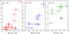 |
Fig. 7 Relations between the normalized line emission intensities IHα (red), IHγ (blue), and IHδ (green) and the color dereddened color excess Δ(J – K)CD mag due to the CD. A black circle surrounds the binary star Nº 5. |
JHK color indices of the studied stars.
Parameters obtained from the fit of the observed Hα emission lines for their CD formation region.
Parameters obtained from the fit of the observed Hγ emission lines for their CD formation region.
Parameters obtained from the fit of the observed Hδ emission lines for their CD formation region.
7.2 The source function
In the frame of an equivalent two-level atom with continuum, the main characteristic of the source functions for the first Balmer lines is that they are strongly dominated by photionizations and radiative recombinations, where collisional ionization and excitation rates can be neglected (Thomas 1957, 1965; Jefferies 1968; Mihalas 1978; Hubeny & Mihalas 2014). The non-LTE source function of these lines are then determined only by the radiation field of the central star. The source function of the first Balmer lines with continuum in an equivalent emitting ring with uniform physical properties can then be approached with the following expressions (Mihalas 1978; Cidale & Ringuelet 1989; Hubeny & Mihalas 2014)
![Mathematical equation: ${S_\lambda }\left( {{\tau _{\rm{o}}}} \right) = \left\{ {\matrix{ {{{\left[ {{\eta \mathord{\left/ {\vphantom {\eta {\left( {1 + \eta } \right)}}} \right. \kern-\nulldelimiterspace} {\left( {1 + \eta } \right)}}} \right]}^{{1 \mathord{\left/ {\vphantom {1 2}} \right. \kern-\nulldelimiterspace} 2}}}B_\lambda ^*} \hfill & {\rm{for}}\,{\tau _o} lt; 1} \hfill \cr {{{\left[ {{\eta \mathord{\left/ {\vphantom {\eta {\left( {1 + \eta } \right)}}} \right. \kern-\nulldelimiterspace} {\left( {1 + \eta } \right)}}} \right]}^{{1 \mathord{\left/ {\vphantom {1 2}} \right. \kern-\nulldelimiterspace} 2}}}B_\lambda ^*\tau _{\rm{o}}^{{1 \mathord{\left/ {\vphantom {1 2}} \right. \kern-\nulldelimiterspace} 2}}} \hfill & {{\rm{for}}\,{\tau _o} \ge 1,} \hfill \cr } } \right.$](/articles/aa/full_html/2023/08/aa46018-23/aa46018-23-eq57.png) (15)
(15)
where we do not consider the thermalization of the source function that should be produced for τo ≳ 10–102. In Eq. (15), τo is the optical depth in the central wavelength of the Balmer λ line; η is the “sink” term in the line source function, S λ; B★ is the “source” factor of S λ. This approximation was already used in Vinicius et al. (2006) and Arias et al. (2007). The expressions for the radiation sink and the source factors η and B★ are given in (Thomas 1965; Hubeny & Mihalas 2014).
In Tables 7–9, the source function ratios S °λ/F★ = [η/(1 + η)]1/2 B★/F★ are given for the Ηα, Ηγ, and Ηδ lines of the studied stars. Within the same framework of radiation-dominated transitions the non-LTE departure coefficients were calculated.
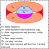 |
Fig. 8 Regions in the disk that contribute in different ways to the observed line emission, according to our simplified representation of the star-disk system. |
7.3 Formal solution of the radiation transfer for the CD
From the simplifications adopted on the geometrical shape of the CD, as a radiation emitting region characterize by a uniform opacity τZ in the direction perpendicular to the equator, can be considered to behave as an equivalent thin ring, having a total height of  and radius R.
Although the simulation of the formation of emission lines from a flat disk of uniform height does not offer particular difficulties (see Horne & Marsh 1986), calculations as a function of the inclination angle, i, in the frame of an equivalent ring are a little more delicate. The shape of the emission ring-region projected towards the observer is sketched in Fig. 8. The radiation field coming from the ring-star system can be represented using the formal solution of the equation of radiation transfer at each point (x, y) projected on the background plane of the sky. For optical depths 0 ≤ τo < 1, according to Eq. (15), the source function S λ = S °λ of the studied Balmer lines is constant. The formal solution of the radiation transfer equation applied to the star-disk system applied to the geometrical configuration given in Fig. 8 is as follows:
![Mathematical equation: $\left. {\matrix{ {I_\lambda ^a\left( {x,y,V - {V_r}} \right) = I_\lambda ^*\left( {x,y} \right)\exp \left[ { - \tau _\lambda ^f{{\left( {x,y,V - {V_r}} \right)} \mathord{\left/ {\vphantom {{\left( {x,y,V - {V_r}} \right)} {\mu \left( {x,y} \right)}}} \right. \kern-\nulldelimiterspace} {\mu \left( {x,y} \right)}}} \right]} \hfill \cr {\,\,\,\,\,\,\,\,\,\,\,\,\,\,\,\,\,\,\,\,\,\,\,\,\,\,\,\,\,\,\,\,\,\,\,\,\,\,\,\, + S{^\circ _\lambda }\left\{ {1 - \exp \left[ { - \tau _\lambda ^f{{\left( {x,y,V - {V_r}} \right)} \mathord{\left/ {\vphantom {{\left( {x,y,V - {V_r}} \right)} \mu }} \right. \kern-\nulldelimiterspace} \mu }\left( {x,y} \right)} \right]} \right\}} \hfill \cr {\,\,\,\,\,\,\,\,\,\,\,\,\,\,\,\,\,\,\,\,\,\,\,\,\,\,\,\,\,\,\,\,\,\,\,\,\,\,\,\,\,\left( {{\rm{stellar}}\,{\rm{emission}}\,{\rm{absorbed}}\,{\rm{by}}\,{\rm{the}}\,{\rm{front}}} \right.} \hfill \cr {\left. {\,\,\,\,\,\,\,\,\,\,\,\,\,\,\,\,\,\,\,\,\,\,\,\,\,\,\,\,\,\,\,\,\,\,\,\,\,\,\,\,\,{\rm{shell}}} \right) + \left( {{\rm{emission}}\,{\rm{from}}\,{\rm{the}}\,{\rm{front}}\,{\rm{shell}}} \right)} \hfill \cr {I_\lambda ^b\left( {x,y,V - {V_r}} \right) = S{^\circ _\lambda }\left\{ {1 - \exp \left[ { - \tau _\lambda ^r - \tau _\lambda ^f{{\left( {x,y,V - {V_r}} \right)} \mathord{\left/ {\vphantom {{\left( {x,y,V - {V_r}} \right)} {\mu \left( {x,y} \right)}}} \right. \kern-\nulldelimiterspace} {\mu \left( {x,y} \right)}}} \right]} \right\}} \hfill \cr {\,\,\,\,\,\,\,\,\,\,\,\,\,\,\,\,\,\,\,\,\,\,\,\,\,\,\,\,\,\,\,\,\,\,\,\,\,\,\,\,\, \times \exp \left[ { - \tau _\lambda ^f{{\left( {x,y,V - {V_r}} \right)} \mathord{\left/ {\vphantom {{\left( {x,y,V - {V_r}} \right)} \mu }} \right. \kern-\nulldelimiterspace} \mu }\left( {x,y} \right)} \right]} \hfill \cr {\,\,\,\,\,\,\,\,\,\,\,\,\,\,\,\,\,\,\,\,\,\,\,\,\,\,\,\,\,\,\,\,\,\,\,\,\,\,\,\, + S{^\circ _\lambda }\left\{ {1 - \exp \left[ { - \tau _\lambda ^f{{\left( {x,y,V - {V_r}} \right)} \mathord{\left/ {\vphantom {{\left( {x,y,V - {V_r}} \right)} \mu }} \right. \kern-\nulldelimiterspace} \mu }\left( {x,y} \right)} \right]} \right\}} \hfill \cr {\,\,\,\,\,\,\,\,\,\,\,\,\,\,\,\,\,\,\,\,\,\,\,\,\,\,\,\,\,\,\,\,\,\,\, = \left( {{\rm{emission}}\,{\rm{from}}\,{\rm{rear}}\,{\rm{shell}}\,{\rm{absorbed}}\,{\rm{by}}} \right.} \hfill \cr {\left. {\,\,\,\,\,\,\,\,\,\,\,\,\,\,\,\,\,\,\,\,\,\,\,\,\,\,\,\,\,\,\,\,\,\,\,\,\,\,\,\,\,\,\,{\rm{front}}\,{\rm{shell}}} \right) + \left( {{\rm{emission}}\,{\rm{by}}\,{\rm{front}}\,{\rm{shell}}} \right)} \hfill \cr } } \right\},$](/articles/aa/full_html/2023/08/aa46018-23/aa46018-23-eq59.png) (16)
(16)
where  is the contribution to the field of radiation by the central star. In these expressions, µ(x, y) is the cosine between the normal to the ring at a test point (x, y) and the sight direction, V is the wavelength displacement in the spectral line in velocity units, and Vr is the radial velocity at the point (x, y), defined below in Sect. 7.4 (Eq. (21)).
For optical depths τo ≥ 1, the formal solution for the radiation field introduces such integrals as:
![Mathematical equation: $\matrix{ {{I_\lambda }} \hfill & = \hfill & {S{^\circ _\lambda }\int_1^{{\tau _o}} {\tau _o^{{1 \mathord{\left/ {\vphantom {1 2}} \right. \kern-\nulldelimiterspace} 2}}\exp \left( { - {\tau _\lambda }} \right){\rm{d}}{\tau _\lambda },} } \hfill \cr {{\tau _\lambda }} \hfill & = \hfill & {{\tau _o}{{\rm{\Phi }}_\lambda },} \hfill \cr {{I_\lambda }} \hfill & = \hfill & {{{\rm{\Phi }}_\lambda }\left[ {\tau _o^{{1 \mathord{\left/ {\vphantom {1 2}} \right. \kern-\nulldelimiterspace} 2}}f\left( {{{\rm{\Phi }}_\lambda }{\tau _o}} \right) - f\left( {{\tau _o}} \right)} \right],} \hfill \cr } $](/articles/aa/full_html/2023/08/aa46018-23/aa46018-23-eq61.png) (17)
(17)
where Φλ is the intrinsic line absorption profile and f(t) is determined by the incomplete gamma function, γ(t, 3/2).
These relations can be used to compose the field of radiation due to overlapping absorbing and emitting layers of the front and rear parts of the equivalent ring. In the optical depths, a distinction is made between  and
and  of the “rear” and “front” layers, respectively, to caution that the radiation field is affected by the Doppler effect. This is due to the possibility of several apparent radial velocity compositions produced by the rotation and expansion velocities of the projected shells relative to the observer.
Finally, the radiation flux in the lines emitted by the star-disk system is given by:
 (18)
(18)
where 𝒮 is the surface of the star-disk system projected onto the sky background, which in addition to the ring surface shown in Fig. 8, encompasses the projected emitting surface of effective cylinder from R to R + ΔR.
The expressions in Eq. (16) can be adapted to several configurations that depend on the value of the height  or
or  and on the value of the inclination angle iRH = arctan(
 ). We previously used this procedure in Floquet et al. (2000), Arias (2004), Vinicius et al. (2006) and Arias et al. (2007).
7.4 Line opacity
We considered the opacity of the studied Balmer lines parameterized according to their value in the Z–direction, which at the respective central wavelength, λo, and in the non-LTE approximation is:
![Mathematical equation: $\matrix{ {{\tau _{{\lambda _o}}} = {\alpha _{{\lambda _o}}}\overline {{N_2}{{\left( R \right)}_Z}} \left\{ {1 - \left( {{{{b_n}} \mathord{\left/ {\vphantom {{{b_n}} {{b_2}}}} \right. \kern-\nulldelimiterspace} {{b_2}}}} \right)\exp \left[ { - \left( {{{hc} \mathord{\left/ {\vphantom {{hc} {{\lambda _o}kT}}} \right. \kern-\nulldelimiterspace} {{\lambda _o}kT}}} \right)} \right]} \right\},} \hfill \cr {{\alpha _{{\lambda _o}}} = {{\left( {\sqrt \pi {e^2}} \right)} \mathord{\left/ {\vphantom {{\left( {\sqrt \pi {e^2}} \right)} {\left( {{m_{\rm{e}}}c} \right)}}} \right. \kern-\nulldelimiterspace} {\left( {{m_{\rm{e}}}c} \right)}}{{\left( {{\lambda _o}f} \right)} \mathord{\left/ {\vphantom {{\left( {{\lambda _o}f} \right)} {\left. {{V_D}} \right)}}} \right. \kern-\nulldelimiterspace} {\left. {{V_D}} \right)}},} \hfill \cr } $](/articles/aa/full_html/2023/08/aa46018-23/aa46018-23-eq68.png) (19)
(19)
where  represents the population of the atomic level n = 2 in the Z– direction, averaged over the radial distance from R to R + ΔR, f is the oscillator strength of the given transition, VD is the total Doppler velocity of its intrinsic absorption line profile that encompasses not only thermal but other possible macroscopic velocity components of statistical nature, and bn represents the non-LTE departure coefficients for atomic levels n. The term (bn/b2)exp[-(hc/λokT)] ≪ 1 can be neglected in most cases.
Writing the line opacity as:
 (20)
(20)
the intrinsic Banner line profile Φ(λ) formally corresponds to the composite expression for a Stark profile given in Gray (2008) or Hubeny & Mihalas (2014). We calculated it using the tables of Stark profiles given by Stehlé & Hutcheon (1999). However, in most cases, the gas density in the disk is low, so that the Stark line broadening is small.
The opacity in the Z–direction, τZ, is adopted in this work as a free parameter. For aspect angles, i ≲ iRH = arctan( ), the optical depth of the shell as a function of the inclination is then parameterized as τ(i) = τZ / cos i and then as τ(i) = τZ tan iRH / sin i when i ≳ iRH. Apart from these i–angle dependencies of the calculated line emission characteristics, stronger inclination angle dependencies are carried by the apparent shape of the entire emission ring-region projected towards the observer, as sketched out in Fig. 8.
The emission intensity at an observed wavelength λ corresponds to the sum of the emissions at wavelength offsets δλ with respect to the central absorption of the atom, which, in turn, is displaced due to the macroscopic movement of the medium with respect to the observer. The absorption (or emission) intensity with which the atom contributes at λ is finally determined by the profile Φ(δλ) = Φ(λ − λo − Δλ), where  and Vr is the total macroscopic radial velocity of the gas at a given point (R, θ) in the ring:
![Mathematical equation: ${V_r} = \left[ {{V_{{\rm{rot}}}}\sin \theta + {V_{\exp }}\cos \theta } \right]\,\sin \,i,$](/articles/aa/full_html/2023/08/aa46018-23/aa46018-23-eq73.png) (21)
(21)
where Vrot is the rotation velocity of the ring and Vexp = Vexpo(Ro/R)α is its “expansion” velocity that is used only to account for the line profile asymmetries. The quantity Vrot is also only to fit at best the width of emission lines, which encompass the actual line broadening by the disk rotation integrated over its formation region and a host of other line broadening mechanisms. Hence, we do not expect to have well defined correlations between Vrot and  .
.
For the line profile calculations we use velocities instead of wavelengths, so that the argument in the profile Φ(λ − λo − Δλ) is readily transformed into velocity displacements [(λ − λo − Δλ)]/ΔλD = (V − Vr)/VD, where V − Vr measures in velocity units the offset λ − λo in the observed profile.
The use of equivalent emitting (absorbing) shell with radius R, also requires a consideration of the Doppler displacements due to the changes of the macroscopic velocity fields in the Z–direction. These contributions are called “shear” components. Following Horne & Marsh (1986), it can be shown that the integrated effect on the line profile of the shear velocity components carries an enlarged line Doppler width ΔλD → ΔD,
![Mathematical equation: ${{\rm{\Delta }}_{\rm{D}}} = {\rm{\Delta }}{\lambda _{\rm{D}}}{\left[ {1 + {{\left( {{{{\lambda _o}} \over {{{\rm{\Delta }}_{{\lambda _{\rm{D}}}}}}}{{{V_{sh}}} \over c}} \right)}^2}} \right]^{{1 \over 2}}},$](/articles/aa/full_html/2023/08/aa46018-23/aa46018-23-eq75.png) (22)
(22)
where the factor in braces acts as a supplementary broadening agent of the line profile. In Eq. (22), Vsh is the contribution of the shear velocity component given by
![Mathematical equation: ${V_{{\rm{sh}}}} = \left[ {{1 \over 2}{V_{{\rm{rot}}}}\sin \theta + \alpha .\,{V_{\exp }}\cos \theta } \right]{{\bar H} \over R}\cos \theta \tan i\sin i.$](/articles/aa/full_html/2023/08/aa46018-23/aa46018-23-eq76.png) (23)
(23)
Shear effects are anisotropic with strong dependence on the inclination angle, i, and azimuth, θ. These effects has almost no incidence on the optically thin lines, but it saturates somewhat the emission peaks as soon as  . In what follows, we assume α = 0. Disks where α ≠ 0, namely, those with gradients of expansion velocities, can be studied using separate equivalent rings which may then reproduce multi-peak emission line profiles (Arias et al. 2007).
7.5 Fit of the line emission components and determination of disk parameters
In our approach the main free parameters are: (1) τZ, the opacity of the ring in the Z–direction; (2) the radius R/Ro of the ring; and (3) the rotation and expansion velocity parameters Vrot and Vexp, respectively. At each iteration step, the extent ΔR of the emitting region in the disk is calculated as a function of the chosen value of R/Ro. We initiate the iterative fitting procedure of the line emission profiles by adopting the calculated value of [η/(1+ η)]1/2 B★/Fc and of  that corresponds to the chosen value of R. In the search for finer adjustments, these quantities can be considered as free parameters. This enables us to test the relevance of the assumptions made on the models of CDs relative to η1/2 B★/Fc and
  . The inclination angle of the star-disk system is taken from Table D.2 already determined with the remaining astrophysical parameters of stars.
All fitting parameters were obtained through a trial-and-error procedure, which is not arbitrary because the global intensity of the emission, the central absorption component in emission lines, and the width of the line wings are sensitive to the ratios between the searched quantities. Nevertheless, we cannot discuss their uniqueness – although it would be possible perhaps if a robust method of adjustment such as the “annealing method” were used (Metropolis et al. 1953). The parameters displayed in Tables 7–9 must then be considered first-order estimates. We note that there are additional uncertainties affecting them which are related to the shape of the emission line profiles proper, mainly when it comes to the extracted ones in Hγ and Hδ lines.
7.6 Extent of the line emission regions
The Gaussian fit of the Ha emission intensity maps obtained with long baseline interferometry for about 20 Be stars (Quirrenbach et al. 1997; Tycner et al. 2004, 2005, 2006, 2008; Koubský et al. 2010; Delaa et al. 2011; Touhami et al. 2013; de Almeida et al. 2020), produce an average observational estimate of the extent of the emission region 〈E/Ro〉 = 7.4 ± 3.5. This value must be compared with our R + ΔR determinations, which for 17 program Be stars lead to the average 〈(R + ΔR)/Ro〉 = 7.4 ± 2.8 that can be considered in good agreement with interferometrical estimates.
7.7 Density distribution in the CD
Only a theory for the CD formation and evolution can determine the function D(R) in Eq. (11) as in VDD model that depends on the chosen viscosity. In this work, we simply assume an analytic expression for D(R) to be valid for the studied line formation region.
In recent interpretations of the photometric, spectroscopic, and polarimetric variations of ω CMa and 66 Oph (Ghoreyshi et al. 2021; Marr et al. 2021), D(R) is characterized in Eq. (11) by a single global exponents, n, that describe the several disk formation phases. These values range from some n ≲ 4.0 at CD formation phases to n ≳ 2.0 at disk dissipation epochs. Nevertheless, much higher values of n may describe the disk formation controlled by periodic mass injection rates, where the injection and dissipation timescales are similar, as shown by Haubois et al. (2012).
For the Hα line formation region, we made the conservative assumption n2 = 3.0 for all program stars, because in our method we cannot determine it otherwise. Since the formation region of the Hα emission component is situated at radii of R ≳ 4Ro, the value of n1 has no incidence on the determination of the hydrogen disk base density ρo g cm−3.
In stars where we could extract reliable emission profiles for the Hy and Hδ lines, we estimated the exponent n1 that characterizes the inner layers of the CD in a relative way by demanding that the values of ρo derived from the optical depths of all three lines be the same and equal to that found with Hα. In Table 10, we give the values of n1 that were thus derived. These values are, on average, 〈n1〉 = 4.3 ± 2.5 – similar to the estimates by Vieira et al. (2017), where n is nevertheless meant to represent the entire radial density distribution at CD forming phases. We can also note that the average [n1 + n2(= 3)]/2 = 3.7 ± 1.3, which is close to the values of n estimated by several authors which used a single n to characterize the entire CD, namely, Silaj et al. (2010), Arcos et al. (2017).
The large variety of n1 values estimated in this work may then correspond to different evolution phases of disks, from their formation to their likely steady state, or dissipation. In cases where spectroscopic observations of Be stars exist only for specific dates, a method such as the one developed in the present work, which is of relative simple use, may still bring useful insights on the nature of CDs. In the present case, the higher values of n1 suggest that in many Be stars the disk formation could respond to periodic mass injection rates, as discussed in Haubois et al. (2012). It is worth noting that further detailed studies of the Hγ and Hδ emission lines at different mass ejection episodes could reveal the physical properties of regions where the viscous transfer of angular momentum is probably organized to the rest of the CD regions and responsible for its Keplerian rotation.
From the radial optical depth τZ, the non-LTE departure coefficients averaged over the respective line formation regions, and assuming that the He abundance in number is roughly NHe ≃ NH/4, we readily determine the CD base density, ρo, which is given in Table 10. These values are of the same order of magnitude than adopted in other more detailed studies (Silaj et al. 2010; Catanzaro 2013; Arcos et al. 2017; Vieira et al. 2017).
The integration of Eq. (11) together with the use of the obtained values of ρo, lead us to an estimate of the total mass, MCD, gathered in the formation regions of the studied Balmer line emissions that are listed in Table 10.
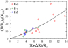 |
Fig. 9 Correlation of Huang’s radii derived with Vrot against line formation extends R + ΔR. In the ordinates the values are from Table 5. |
7.8 Additional comments on the CDs
Our CD emission model is challenged with the star n = 5. This object is a binary system, where it is likely that contributions by two distinct regions in the disk would be needed to account for the entire Ha line emission profile in a more reliable way.
Arcos et al. (2017) obtained a correlation at 61% between Huang’s radii and the radii R90, which represents the distance in the CD up to which 90% of the line emission is formed. We note that the V sin i parameters used to this end were not measured, but obtained as one among several parameters used to fit the Hα emission line profiles. We obtain a similar correlation at 68% between Huang’s radii calculated with the fitting quantity Vrot and then distance R + ΔR (see Fig. 9). However, because in both approaches Huang’s radii are calculated with fitted rotational velocities, doubts can be cast on the physical reliability of these correlations.
Then, Vexp is a fitting parameter needed to account for the line emission asymmetry. It resumes perhaps the effects carried by the known quasi-cyclic V/R variations attributed to the global one-armed disk density oscillations (Kato 1983; Okazaki 1991, 1997).
Finally, in this work we did not attempt to interpret the correlations implying emission lines and photometric measurements, simply because it would require to include a study of the formation of the continuum energy distribution with approaches like those carried by Moujtahid (1998), Moujtahid et al. (2000a,b), which are not in the scope of the present paper.
8 Discussions
8.1 Comments on the pnrc parameters
A rotating star of mass, M, behaves as an object with lower effective mass M − ΔM, where ΔM is proportional to the pressure-weighted average of the centrifugal to the gravitational force over the entire object (Sackmann 1970; Clement 1979). Consequently, the rotating star produces a lower bolometric luminosity during roughly the first half of the main sequence (MS) evolutionary phase and has longer evolving time scales than its non-rotating counterpart. Rotational mixing carries fresh H-fuel into the convective core, which still prolongs its life in the MS phase (Maeder & Meynet 2000). This mixing also transports helium (and other H-burning products) into the radiative envelope, which lowers its opacity and contributes to the enhancement of the emitted stellar luminosity over that produced by the non-rotating objet with same mass, taking place near to the second half of the MS phase (Maeder 2009).
The apparent luminosity depends mainly on the geometrical deformation of the star, the gravitational darkening effect (GD) and the inclination angle at which is seen the object. Generally, the GD effect produces an average lower apparent effective temperature and the geometrical deformation of the star leads to an apparent average lower effective gravity. This explains that the pnrc effective temperatures and gravities are larger than the apparent ones. Concerning the bolometric luminosity, the picture is less clear and strongly depends on the combination of the astrophysical parameters, mainly on the rotation rate and on the stellar aspect angle. Roughly, the ratio of the apparent to the pnrc bolometric luminosity is ![Mathematical equation: ${L^{{\rm{app}}}}{{\left( {i,\Omega } \right)} \mathord{\left/ {\vphantom {{\left( {i,\Omega } \right)} {{L^{{\rm{pnrc}}}}}}} \right. \kern-\nulldelimiterspace} {{L^{{\rm{pnrc}}}}}} \simeq \left[ {S{{\left( {i,\Omega } \right)} \mathord{\left/ {\vphantom {{\left( {i,\Omega } \right)} {{S_{{\rm{pnrc}}}}}}} \right. \kern-\nulldelimiterspace} {{S_{{\rm{pnrc}}}}}}} \right]{\left[ {{{\left\langle {T_{{\rm{eff}}}^{{\rm{app}}}\left( {i,\Omega } \right)} \right\rangle } \mathord{\left/ {\vphantom {{\left\langle {T_{{\rm{eff}}}^{{\rm{app}}}\left( {i,\Omega } \right)} \right\rangle } {T_{{\rm{eff}}}^{{\rm{pnrc}}}}}} \right. \kern-\nulldelimiterspace} {T_{{\rm{eff}}}^{{\rm{pnrc}}}}}} \right]^4}$](/articles/aa/full_html/2023/08/aa46018-23/aa46018-23-eq80.png) , where “S” is the area of the apparent stellar hemisphere and that of the non-rotating counterpart, respectively. In this relation we take the effective temperature of the rotating object averaged over the deformed observed stellar hemisphere. See details on the behavior of Lapp(i, Ω) and
, where “S” is the area of the apparent stellar hemisphere and that of the non-rotating counterpart, respectively. In this relation we take the effective temperature of the rotating object averaged over the deformed observed stellar hemisphere. See details on the behavior of Lapp(i, Ω) and  in Zorec et al. (2016). The conditions Lpnrc ≳ Lapp(i, Ω) or Lpnrc ≲ Lapp(i, Ω) are controlled by the competition between S (i,Ω) and
  . The apparent Vsin i parameter is underestimated because the equatorial regions, which have the larger surface linear rotational velocities, reduce their contribution to the rotational line broadening due to the GD effect. A comparison between the pnrc parametric set (Vsin i, Teff, log g, log L/L⊙) obtained for Ω/Ωc = 0.95, with the apparent one is shown in Fig. 10.
A test on the reliability of the pnrc parameters can be done by comparing the pnrc stellar masses with the masses obtained using detached binary systems. The pnrc stellar masses are meant to represent the actual ones. This comparison is shown in Fig. 11. The blue points are for masses determined using the apparent astrophysical parameters and the red ones are for masses determined with the pnrc parameters. In this figure, the average (log M/M⊙, log Teff) relations are from Harmanec (1988, green curves) and from Xiong et al. (2023, brown curves), with the latter obtained in the frame of the LAMOST medium-resolution spectroscopic survey. We see that the pnrc masses closely lie, within the uncertainty strips, around the mean relation of masses measured in detached binary systems.
In principle, an O-, B- or A-type star may acquire the required properties to display the Be phenomenon in several ways. It may be due to: formation and pre-main sequence evolution circumstances of single stars; internal angular momentum evolution properties during the MS phase (see references in Zorec 2023); a rejuvenating process as a consequence that one of the components has gained mass and angular momentum during mass transfer phases in binary systems (Packet 1981; Pols et al. 1991; de Mink et al. 2013). Depending on the several circumstances that may characterize the mass transfer phenomenon, the resulting Be stars should be binaries or single stars (Shao & Li 2014; Hastings et al. 2021). If they are binaries, their companions can be stripped sub-dwarf O/B (sdO/B) He stars (BeHe), white dwarfs (BeWD, neutron stars (BeNS), or black holes (BeBH). Single Be stars can be merger objects (Bemerger), disrupted BeNS or BeBH binaries. A significant number of recent observational data show that Be stars are binaries indeed, where the secondary is probably a stripped sdO/B object (Bodensteiner et al. 2020; El-Badry et al. 2022, and references therein). The paradigm of mass transfer may perhaps explain the nature of the star N° 5 studied in this paper and that we briefly discuss in Sect. 8.2.
From the above-cited set of possible companions of Be stars in binary system, those whose presence was neglected in the present work but may in principle have some effect on the Teff determination include: white dwarfs and the stripped sdO/B companions. However, as white dwarfs have radii of RWD/R⊙ = 0.01(M⊙/MWD)1/3, masses of 0.15 ≲ MWD/MWD ≲ 1.4, and effective temperatures of  , they can hardly carry any effect on the estimated Teff of our program Be stars. This may not be the case with hot sub-dwarf companions. According to Heber (2009), hot sub-dwarfs have most frequently effective temperatures in the range of
  , and radii in the interval 0.15 ≲ Rsd/R⊙ ≲ 0.25. If we neglect their presence, the extreme errors that we will risk to commit on the estimate of the apparent effective temperatures of Be stars, can be estimated using the following extreme approximate bolo-metric luminosity relations, namely, both stars are seen or the sdO/B eclipses the Be star:
  and
and  , where TBe, TB and Tsd are: the effective temperature obtained with GIRFIT of the studied Be star, the actual effective temperature expected for the Be star, and the effective temperature of the sub-dwarf, respectively; the sB and ssd represent the areas of the Be and sub-dwarf respective apparent stellar surfaces. Because r = ssd/sB ≪ 1, we have for both cases TB ≈ TBe × {[1 − r(Tsd/TBe)4]}, which applied individually to our program objects enables us to estimate the effective temperature and the radius of the sub-dwarf star that carry on the Teff estimate an error on the order of the uncertainty characterizing our effective temperature determinations. The average effective temperature and radius of sdO/B stars thus calculated are: 〈Tsd〉 = 43 600 ± 13 000 K and 〈Rsd/R⊙〉 = 0.27 ± 0.06, respectively. According to these results, the sdO/B stars in our sample should belong to the largest and hottest population of sdO/B stars. Such objects would certainly leave spectral signatures in the wavelength region studied in this work by He II λλ 4100, 4200, 4338, CIV λ 4442 and NIII λ 4379 lines (Drilling et al. 2013), which are not obvious to identify in our spectra with certainty. We may then conclude that if these sdO/B are proven to exist, their effect on the Teff determinations will be at most of the order of uncertainties inherent to the spectral resolutions and S/Ns used in this work. However, star N° 5 decidedly requires a detailed study of the actual nature of the secondary, which (according to the characteristics of eclipses) could be larger than those considered in the above estimates.
It is worth recalling that the Be phenomenon proper remains linked to the physical characteristics of the O-, B- or A-type star, whatever the origin of Be stars as either single or merger byproducts. However, when dealing with binary systems, precise determinations of the astrophysical parameters of Be stars still requires that from now on it would be wise to carry out a thorough inquiry on the presence of companions and and on their characteristics, as well as on their perturbation power on the energy distribution of the primary in the studied spectral interval.
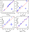 |
Fig. 10 Comparison between the pnrc parametric set (Vsin i, Teff, log g, log L/L⊙) obtained for Ω./Ωc = 0.95 with the apparent one. The average uncertainties of the plotted quantities are indicated. The diagonal in red represents the identity relation. |
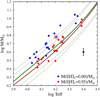 |
Fig. 11 Comparison of Be stellar masses obtained in this paper with those of non-Be stars against the effective temperature. Blue dots represent the masses obtained from the apparent astrophysical parameters. Red dots represent the pnrc stellar masses determined for Ω/Ωc = 0.95. The green curve and the dotted green lines represent the average empirical relation curve with the error margins obtained by Harmanec (1988, |


8.2 The binary star N° 5
The astrophysical parameters of the star N° 5 were determined assuming that the object was a single star, although the light curve clearly indicates that it is a close eclipsing binary system (Klagyivik et al. 2017). Neglecting the presence of the companion and the perturbations that it may introduce to the SED of the primary would lead us to infer the improbable inclination angle for the primary i ~ 50° if Ω/Ωc = 0.95. In fact, we could expect that the most probable inclination should be close to i ~ 90°, because we are dealing with an eclipsing binary. However, assuming i ~ 90° and consequently fixing the value of the rotation parameter of the primary at V sin i = 337 km s−1, the GIRFIT fitting procedure produces bad adjustments of the synthetic spectra with the observed ones, and ends up with the following estimates of the apparent astrophysical parameters: Teff = 14 000 ± 700 K and log g = 3.20 ± 0.16.
Moreover, the Ha emission line has likely a shell aspect. Other shell signatures are also found in the unique spectrum at our disposal (He I 6678 and 7065 Å). Unfortunately, the scarce data we have on this star do not help in determining whether the shell features are produced by a circumstellar disk or whether they are signatures attributed to the secondary component.
Due to the combined effect of gravitational and centrifugal forces, the circumstellar disk of the Be component will tend to be on or around its equatorial plane and probably near or over the binary orbital plan. However, we cannot give in to the temptation of speculating on a possible complex circumbinary envelope deploying strongly outside the binary plane, produced by a mass transfer episode between the components, such as those recently predicted by Smallwood et al. (2023). Such complex circumbinary gaseous structures can lead to misinterpretations of the position (inclination) of the circumstellar disk of the Be star.
8.3 Considering the rotational velocity rates
Regarding the corrections of effects carried by the rapid rotation on the apparent astrophysical parameters, we note that if we had enough independent apparent parameters as in the case of the calculations presented in Frémat et al. (2005) or Zorec et al. (2016), we could produce an estimate of the actual rotation frequency for each star individually. Since in this paper we do not have the required number of independent entry parameters, we ought to parameterize the ratios Ω/Ωc.
Thus, we considered only the two extreme cases Ω/Ωc = 0.0 and 1.0, for which the average velocity ratios corrected for GD effects are 〈V/Vc〉 = 0.85 ± 0.20 and 〈V sin i/Vc〉 = 0.91 ± 0.20, respectively. In turn, these ratios correspond to (Ω/Ωc) = 0.96 ± 0.10 and (Ω/Ωc) = 0.99 ± 0.05, or to equatorial force ratios (η = Fcentrifugal/Fgravity) = 0.64 ± 0.33 and 〈η〉 = 0.77 ± 0.29, respectively. Thus, the force ratios clearly indicate that on average our stars have quite under-critical rotations, even though the average Ω/Ωc ratios seem to suggest otherwise (see Zorec et al. 2016; Zorec 2023).
The obtained rotation rates can be translated into ratios of rotational frequencies that are in the interval 〈νr(Ω/Ωc = 1.0)/νr(Ω/Ωc = 0.95)〉 = 1.10 ± 0.02. This range can be taken as an indicator of the uncertainties affecting the rotational frequencies due to possible undue choices of the individual Ω/Ωc values.
9 Concluding remarks
A set of faint 19 B-type stars of which 18 are Be stars, observed by the satellite CoRoT in the fourth long run (LRA02), was studied by spectroscopy. Using spectra in the λλ 4000-4500 Å obtained during a spectroscopic campaign with the VLT/FLAMES instruments at ESO. When necessary, the SEDs of Be stars were corrected for the veiling effect due to the circumstellar disk emission. All studied stars were assumed to be single stars or their SEDs had not been perturbed in the analyzed spectral range by the presence of possible stripped sdO/B components produced during the mass transfer phase in binary systems.
The fit of spectra with models of stellar atmospheres using our GIRFIT package based on the MINUIT minimization algorithm developed by CERN, produced apparent astrophysical parameters of stars, which were then corrected for the effects induced by the rapid rotation according to parameterized ratios Ω/Ωc The corrected astrophysical parameters enabled us to estimate true rotation frequencies that will be used in a following paper dealing with the analysis of non-radial pulsations derived from the light curves observed by CoRoT. We have concluded that it is difficult to decide whether the estimated effective temperatures in this work are systematically affected by the presence of sub-dwarf companions, because the expected mis-estimate of the effective temperatures depend on the actual characteristics of the companion sdO/B stars, and that they could be on the order of uncertainties related to the resolution and S/Ns of the spectra analyzed.
The masses of stars derived with the pnrc astrophysical parameters and models of stellar evolution are in agreement with the masses measured in detached binary systems. Moreover, the obtained astrophysical parameters faithfully reproduce the stellar distances measured by Gaia.
We note however, that the inclination angle and other astrophysical parameters of the star Nº 5 remain uncertain because in this case, the perturbation due to the secondary could be not negligible. Unfortunately, we do not have enough data to study this issue and decide whether some spectral features are genuine spectroscopic shell characteristics or they are signatures due to the presence a binary component.
Using the pnrc astrophysical parameters lead us to conclude that the studied Be stars are rapid rotators, but the relation of the equatorial centrifugal force to the gravity indicate that they are far from being critical rotators. Critical or near-critical rotation is a necessary ingredient to favor massive mass ejections related with the non-radial pulsations (Kee et al. 2016). Nevertheless, the inferred Ω/Ωc: ratios are large enough to favor the appearance of more or less extended regions in the stellar envelope and in the sub-photospheric regions that become unstable to convection (Clement 1979; Maeder et al. 2008; Cantiello et al. 2009). Since convection favors the setting out of differential rotation with a concomitant production of internal magnetic fields, magnetic dynamos, and cyclic activities (Zorec et al. 2011; Zorec 2023; Keszthelyi 2023), we may ask whether instabilities related with these magnetic fields could be the cause of significant upheavals in the outer stellar structure, where the correlated non-radial pulsations and huge sporadic mass ejections could both be phenomena triggered by these disturbances. In the framework of this phenomenology, the study of non-radial pulsations in Be stars may acquire a new major area of interest centered on the study of the internal structure of rapidly rotating stars.
Spectra were obtained also in the region of the Hα line to confirm the Be nature of objects in the chosen set of stars. For some objects, emission components could also be extracted in the Hγ and Hδ lines. Using a simplified representation of the line emitting regions in a flat CD, we inferred indications on the physical properties of disks surrounding the observed Be stars. A non-LTE approach was employed to calculate the source function of lines and their opacity based on first principles that control the level populations of atoms. Entrusting the fit obtained of the observed Hα, Hγ, and Hδ emission lines profiles with model CD disks oriented according to the inclination angles derived from the astrophysical parameters, we have discussed the density distribution in the CDs. We thus found that the exponent of the density distribution in the radial direction of the circumstellar disk is a function of the distance, R.
Although the VDD models also predict exponents of the radial distribution of the density in the CDs that depend on the distance, our results point out on the necessity to carry out controls of the predicted exponents using detailed analysis of spectral lines that preferentially form in regions close to the central object. These regions are fed with material by sporadic huge mass ejections and variable stellar winds that provide the material to build up the CD. The spectral lines formed in these regions may reveal the actual physical properties of layers which make the transition from the star to the CD and where is organized the transport of the angular momentum that in fine determines the Keplerian rotation of disks in Be stars.
The obtained extents of the Hα line emission formation regions are in agreement with similar quantities estimated elsewhere by interferometry in other Be stars. From the derived line opacity, we inferred the CD base densities that closely approach those estimated with much detailed models developed recently by other authors. Assuming that the snapshot image brought by our spectra of the line emission profiles can be attributed to a kind of stationary structure of the CD, the disk base density enabled us to obtain a rough estimate of the mass contained in the region of the line formation regions. These estimates are also in good agreement with other published estimates in the literature, where they were derived considering that the CD are subject to a dynamical evolution as well as that a quasi stationary picture actually results from several mass injection phenomena and to their dissipation.
Program ID : 086.D-0212(A), (PI: C. Neiner).
Acknowledgements
This work has made use of data from the European Space Agency (ESA) mission Gaia (https://www.cosmos.esa.int/gaia), processed by the Gaia Data Processing and Analysis Consortium (DPAC, https://www.cosmos.esa.int/web/gaia/dpac/consortium). Funding for the DPAC has been provided by national institutions, in particular the institutions participating in the Gaia Multilateral Agreement. This research has made use of the service of the ESO Science Archive Facility. We are thankful to the referee for his/her attentive reading of the manuscript and for his/her many suggestions and corrections that improved the presentation of our results.
Appendix A Table containing the information on FLAMES/GIRAFFE spectra and conditions of their exposure time
Log of the stars observed with FLAMES/GIRAFFE
Appendix B Comparison between an observed and the corresponding veiling corrected spectrum
According to Semaan et al. (2013), the expression to correct the spectra for the veiling effect is
![Mathematical equation: $\left. {\matrix{ {{F^*}{{\left( \lambda \right)} \mathord{\left/ {\vphantom {{\left( \lambda \right)} {F_{\rm{c}}^*}}} \right. \kern-\nulldelimiterspace} {F_{\rm{c}}^*}}\left( \lambda \right) = \left\{ {\left[ {{F^{{\rm{obs}}}}{{\left( \lambda \right)} \mathord{\left/ {\vphantom {{\left( \lambda \right)} {F_{\rm{c}}^{{\rm{obs}}}\left( \lambda \right)}}} \right. \kern-\nulldelimiterspace} {F_{\rm{c}}^{{\rm{obs}}}\left( \lambda \right)}}} \right]\,\left[ {1 + r\left( \lambda \right)} \right] - r\left( \lambda \right)} \right\}} \hfill \cr {\,\,\,\,\,\,\,\,\,\,\,\,\,\,\,\,\,\,\,\,\,\,r\left( \lambda \right) = {E_{\rm{c}}}{{\left( \lambda \right)} \mathord{\left/ {\vphantom {{\left( \lambda \right)} {\left[ {F_{\rm{c}}^*\left( \lambda \right){A_{\rm{c}}}\left( \lambda \right)} \right]}}} \right. \kern-\nulldelimiterspace} {\left[ {F_{\rm{c}}^*\left( \lambda \right){A_{\rm{c}}}\left( \lambda \right)} \right]}}} \hfill \cr } } \right\},$](/articles/aa/full_html/2023/08/aa46018-23/aa46018-23-eq87.png) (B.1)
(B.1)
where Fobs(λ) is the observed line spectrum;  is the continuum spectrum emitted by the star+disk system; F★(λ) and
  are the line and continuum spectra due to the stellar photosphere, respectively. The term “1 + r” is called the “veiling factor.” Ec(λ) and Ac(λ) respectively represent the amount of continuum emission and absorption due to the CD that can be estimated using the empirical correlations in (Ballereau et al. 1995). The veiling factor in Eq. (B.1) is a function of λ that varies by Δr/r > 0.04 from λ = 4000 Å to λ = 4500 Å as it can be inferred from relations given in Moujtahid et al. (1999, 2000a) and using the required parameters calculated in Zorec et al. (2016). The term r(λ) roughly behaves as r(λ) = a × (λ/λHγ)3 + b. Frémat et al. (2006) showed that by neglecting the veiling effect in Be stars displaying strong line emissions, the determination of astrophysical parameters (Teff, log g) may suffer from substantial uncertainties. The veiling factors r at λ = 4500 Å determined using the empirical correlations in Ballereau et al. (1995) and the emission intensities IHγ in the Hγ line are given in Table B.1. The emission intensity in the Hγ line is defined as
 ![Mathematical equation: ${I_{{\rm{H}}\gamma }} = W_{{\rm{H}}\gamma }^{{\rm{em}}} \times \left\{ {{{\left[ {F_{{\rm{H}}\gamma }^{\rm{c}}\left( {{T_{{\rm{eff}}}},\log g} \right)} \right]} \mathord{\left/ {\vphantom {{\left[ {F_{{\rm{H}}\gamma }^{\rm{c}}\left( {{T_{{\rm{eff}}}},\log g} \right)} \right]} {\left[ {F_{{\rm{H}}\gamma }^{\rm{c}}\left( {22500,4.0} \right)} \right]}}} \right. \kern-\nulldelimiterspace} {\left[ {F_{{\rm{H}}\gamma }^{\rm{c}}\left( {22500,4.0} \right)} \right]}}} \right\}$](/articles/aa/full_html/2023/08/aa46018-23/aa46018-23-eq90.png) , where
, where  represents the equivalent width of the emission component of the Hy line and
  is the flux of the continuum spectrum at Hy. In Table B.1, stars Nº 1, 6, 12, and 16 have very low emission and accordingly it is r ≃ 0. An example of the effect introduced on spectra by the correction by the veiling effect is shown in Fig. B.1.
As an example of spectra before and after correction made for the veiling effect are shown in Fig. B.1. They correspond to the Be star ID 300002611 (Nº 17). The correction is made over the entire spectral range of λλ4000 – 4500 Å. The spectra in Fig. B.1 are shown to be arbitrarily shifted in the ordinates. In this figure is also shown the difference between the observed and veiling corrected spectra to appreciate the change in the equivalent widths of spectral lines and the almost negligible variation introduced on the energy distribution in the treated wavelength interval.
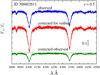 |
Fig. B.1 Comparison between normalized observed and veiling corrected spectra of the program star Nº 17 (ID 300002611) in the wavelength interval λλ 4000 – 4500 Å. |
Equivalent width and normalized flux of the emission component in the H line, and the veiling factor 1 + r.
Appendix C Spectra in the blue region and the obtained best fits
Appendix D Astrophysical parameters and rotational frequencies corrected for rotational effects of the observed Be stars assuming the angular velocity ratio Ω/Ωc = 0.95
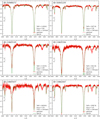 |
Fig. C.1 Observed spectra corrected for veiling effects of the program stars from N° 1 to 6 in the wavelength interval λλ 4000 – 4500 Å. |
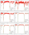 |
Fig. C.2 Observed spectra corrected for veiling effects of the program stars from No 7 to 12 in the wavelength interval λλ 4000 – 4500 Å. |
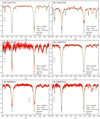 |
Fig. C.3 Observed spectra corrected for veiling effects of the program stars from N° 13 to 18 in the wavelength interval λλ 4000 – 4500 Å. |
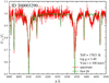 |
Fig. C.4 Observed spectra corrected for veiling effects of the program star Nº 19 in the wavelength interval λλ 4000–4500 Å. |
Averaged astrophysical parameters and rotational frequencies corrected for rotational effects of the observed Be stars assuming the angular velocity ratio Ω/Ωc = 0.95
Modes of astrophysical parameters and rotational frequencies corrected for rotational effects of the observed Be stars assuming the angular velocity ratio Ω/Ωc = 0.95
References
- Arcos, C., Jones, C. E., Sigut, T. A. A., Kanaan, S., & Curé, M. 2017, ApJ, 842, 48 [NASA ADS] [CrossRef] [Google Scholar]
- Arias, M. L. 2004, PhD thesis, National University of La Plata, Argentina [Google Scholar]
- Arias, M. L., Zorec, J., & Frémat, Y. 2007, ASP Conf. Ser., 361, 419 [NASA ADS] [Google Scholar]
- Ashok, N. M., Bhatt, H. C., Kulkarni, P. V., & Joshi, S. C. 1984, MNRAS, 211, 471 [NASA ADS] [CrossRef] [Google Scholar]
- Baade, D., Rivinius, T., Pigulski, A., et al. 2016, A&A, 588, A56 [NASA ADS] [CrossRef] [EDP Sciences] [Google Scholar]
- Baglin, A., Auvergne, M., Barge, P., et al. 2006, ESA SP, 1306, 33 [NASA ADS] [Google Scholar]
- Ballereau, D., Chauville, J., & Zorec, J. 1995, A&AS, 111, 423 [NASA ADS] [Google Scholar]
- Basri, G., & Batalha, C. 1990, ApJ, 363, 654 [Google Scholar]
- Bodensteiner, J., Shenar, T., & Sana, H. 2020, A&A, 641, A42 [NASA ADS] [CrossRef] [EDP Sciences] [Google Scholar]
- Borucki, W. J., Koch, D., Basri, G., et al. 2010, Science, 327, 977 [Google Scholar]
- Burssens, S., Simón-Díaz, S., Bowman, D. M., et al. 2020, A&A, 639, A81 [NASA ADS] [CrossRef] [EDP Sciences] [Google Scholar]
- Cantiello, M., Langer, N., Brott, I., et al. 2009, A&A, 499, 279 [NASA ADS] [CrossRef] [EDP Sciences] [Google Scholar]
- Carciofi, A. C., & Bjorkman, J. E. 2006, ApJ, 639, 1081 [Google Scholar]
- Carciofi, A. C., & Bjorkman, J. E. 2008, ApJ, 684, 1374 [Google Scholar]
- Castelli, F., & Kurucz, R. L. 2003, IAU Symp., 210, A20 [Google Scholar]
- Castelli, F., Gratton, R. G., & Kurucz, R. L. 1997, A&A, 318, 841 [NASA ADS] [Google Scholar]
- Catanzaro, G. 2013, A&A, 550, A79 [NASA ADS] [CrossRef] [EDP Sciences] [Google Scholar]
- Chauville, J., Zorec, J., Ballereau, D., et al. 2001, A&A, 378, 861 [NASA ADS] [CrossRef] [EDP Sciences] [Google Scholar]
- Cidale, L. S., & Ringuelet, A. E. 1989, PASP, 101, 417 [NASA ADS] [CrossRef] [Google Scholar]
- Clement, M. J. 1979, ApJ, 230, 230 [CrossRef] [Google Scholar]
- Collins, I., George, W., 1987, IAU Colloq., 92, 3 [NASA ADS] [Google Scholar]
- Cook, K. H., Alcock, C., Allsman, H. A., et al. 1995, ASP Conf. Ser., 83, 221 [NASA ADS] [Google Scholar]
- Cox, A. N. 2000, Allen’s Astrophysical Quantities (UK: The University of London, The Athlone Press) [Google Scholar]
- Cranmer, S. R. 2005, ApJ, 634, 585 [NASA ADS] [CrossRef] [Google Scholar]
- Cutri, R. M., Skrutskie, M. F., van Dyk, S., et al. 2003, 2MASS All Sky Catalog of point sources (NASA/IPAC) [Google Scholar]
- Dachs, J., Engels, D., & Kiehling, R. 1988, A&A, 194, 167 [NASA ADS] [Google Scholar]
- de Almeida, E. S. G., Meilland, A., Domiciano de Souza, A., et al. 2020, A&A, 636, A110 [NASA ADS] [CrossRef] [EDP Sciences] [Google Scholar]
- de Jager, C., & Neven, L. 1959, The Observatory, 79, 102 [NASA ADS] [Google Scholar]
- de Mink, S. E., Langer, N., Izzard, R. G., Sana, H., & de Koter, A. 2013, ApJ, 764, 166 [Google Scholar]
- de Wit, W. J., Lamers, H. J. G. L. M., Marquette, J. B., & Beaulieu, J. P. 2006, A&A, 456, 1027 [NASA ADS] [CrossRef] [EDP Sciences] [Google Scholar]
- Delaa, O., Stee, P., Meilland, A., et al. 2011, A&A, 529, A87 [NASA ADS] [CrossRef] [EDP Sciences] [Google Scholar]
- Deleuil, M., Moutou, C., Cabrera, J., et al. 2016, in The CoRoT Legacy Book: he Adventure of the Ultra High Precision Photometry from Space (France: EDP Sciences), 117 [CrossRef] [Google Scholar]
- Drilling, J. S., Jeffery, C. S., Heber, U., Moehler, S., & Napiwotzki, R. 2013, A&A, 551, A31 [NASA ADS] [CrossRef] [EDP Sciences] [Google Scholar]
- El-Badry, K., Conroy, C., Quataert, E., et al. 2022, MNRAS, 516, 3602 [NASA ADS] [CrossRef] [Google Scholar]
- Espinosa Lara, F., & Rieutord, M. 2011, A&A, 533, A43 [NASA ADS] [CrossRef] [EDP Sciences] [Google Scholar]
- Floquet, M., Hubert, A. M., Hirata, R., et al. 2000, A&A, 362, 1020 [NASA ADS] [Google Scholar]
- Flower, P. J. 1996, ApJ, 469, 355 [NASA ADS] [CrossRef] [Google Scholar]
- Frémat, Y., Zorec, J., Hubert, A. M., & Floquet, M. 2005, A&A, 440, 305 [NASA ADS] [CrossRef] [EDP Sciences] [Google Scholar]
- Frémat, Y., Neiner, C., Hubert, A. M., et al. 2006, A&A, 451, 1053 [NASA ADS] [CrossRef] [EDP Sciences] [Google Scholar]
- Gaia Collaboration (Prusti, T., et al.) 2016, A&A, 595, A1 [NASA ADS] [CrossRef] [EDP Sciences] [Google Scholar]
- Gaia Collaboration (Brown, A. G. A., et al.) 2021, A&A, 649, A1 [NASA ADS] [CrossRef] [EDP Sciences] [Google Scholar]
- Gaia Collaboration (Vallenari, A., et al.) 2023, A&A, 674, A1 [NASA ADS] [CrossRef] [EDP Sciences] [Google Scholar]
- Galazutdinov, G. A., Musaev, F. A., Krełowski, J., & Walker, G. A. H. 2000, PASP, 112, 648 [NASA ADS] [CrossRef] [Google Scholar]
- Georgy, C., Ekström, S., Granada, A., et al. 2013, A&A, 553, A24 [NASA ADS] [CrossRef] [EDP Sciences] [Google Scholar]
- Ghoreyshi, M. R., Carciofi, A. C., Rímulo, L. R., et al. 2018, MNRAS, 479, 2214 [Google Scholar]
- Ghoreyshi, M. R., Carciofi, A. C., Jones, C. E., et al. 2021, ApJ, 909, 149 [NASA ADS] [CrossRef] [Google Scholar]
- Gkouvelis, L., Fabregat, J., Zorec, J., et al. 2016, A&A, 591, A140 [NASA ADS] [CrossRef] [EDP Sciences] [Google Scholar]
- Goss, K. J. F., Karoff, C., Chaplin, W. J., Elsworth, Y., & Stevens, I. R. 2011, MNRAS, 411, 162 [NASA ADS] [CrossRef] [Google Scholar]
- Granada, A., Arias, M. L., & Cidale, L. S. 2010, AJ, 139, 1983 [Google Scholar]
- Gray, D. F. 2008, The Observation and Analysis of Stellar Photospheres (Cambridge: Cambridge University Press) [Google Scholar]
- Grevesse, N., & Sauval, A. J. 1998, Space Sci. Rev., 85, 161 [Google Scholar]
- Hanuschik, R. W. 1989, Ap&SS, 161, 61 [NASA ADS] [CrossRef] [Google Scholar]
- Hanuschik, R. W. 2003, A&A, 407, 1157 [NASA ADS] [CrossRef] [EDP Sciences] [Google Scholar]
- Harmanec, P. 1988, Bull. Astron. Inst. Czechoslovakia, 39, 329 [Google Scholar]
- Hastings, B., Langer, N., Wang, C., Schootemeijer, A., & Milone, A. P. 2021, A&A, 653, A144 [NASA ADS] [CrossRef] [EDP Sciences] [Google Scholar]
- Haubois, X., Carciofi, A. C., Rivinius, T., Okazaki, A. T., & Bjorkman, J. E. 2012, ApJ, 756, 156 [Google Scholar]
- Hawkins, F. M. 1961, MNRAS, 122, 285 [NASA ADS] [Google Scholar]
- Heber, U. 2009, ARA&A, 47, 211 [Google Scholar]
- Hernández, J., Calvet, N., Hartmann, L., et al. 2005, AJ, 129, 856 [CrossRef] [Google Scholar]
- Horne, K., & Marsh, T. R. 1986, MNRAS, 218, 761 [NASA ADS] [CrossRef] [Google Scholar]
- Huang, S.-S. 1972, ApJ, 171, 549 [NASA ADS] [CrossRef] [Google Scholar]
- Huat, A.-L., Hubert, A.-M., Baudin, F., et al. 2009, A&A, 506, 95 [NASA ADS] [CrossRef] [EDP Sciences] [Google Scholar]
- Hubeny, I., & Lanz, T. 1995, ApJ, 439, 875 [Google Scholar]
- Hubeny, I., & Mihalas, D. 2014, Theory of Stellar Atmospheres (Princeton: Princeton Series in Astrophysics) [Google Scholar]
- Hubert, A. M., & Floquet, M. 1998, A&A, 335, 565 [NASA ADS] [Google Scholar]
- Hubert-Delplace, A. M., Hubert, H., Ballereau, D., & Chambon, M. T. 1982, IAU Symp., 98, 195 [NASA ADS] [Google Scholar]
- Hummel, W. 1994, A&A, 289, 458 [NASA ADS] [Google Scholar]
- Jackson, B. V., Buffington, A., Hick, P. P., et al. 2004, Sol. Phys., 225, 177 [NASA ADS] [CrossRef] [Google Scholar]
- Jaschek, M., Slettebak, A., & Jaschek, C. 1981, Be Star Newslett., 4, 9 [NASA ADS] [Google Scholar]
- Jefferies, J. T. 1968, Spectral line formation (Waltham: Blaisdell Publishing Company) [Google Scholar]
- Jenniskens, P., & Desert, F. X. 1994, A&AS, 106, 39 [NASA ADS] [Google Scholar]
- Kastner, J. H., & Mazzali, P. A. 1989, A&A, 210, 295 [NASA ADS] [Google Scholar]
- Kato, S. 1983, PASJ, 35, 249 [NASA ADS] [Google Scholar]
- Kee, N. D., Owocki, S., Townsend, R., & Müller, H. R. 2016, ASP Conf. Ser., 506, 47 [Google Scholar]
- Keller, S. C., Bessell, M. S., Cook, K. H., Geha, M., & Syphers, D. 2002, AJ, 124, 2039 [Google Scholar]
- Keszthelyi, Z. 2023, Galaxies, 11, 40 [NASA ADS] [CrossRef] [Google Scholar]
- Kinman, T., & Castelli, F. 2002, A&A, 391, 1039 [NASA ADS] [CrossRef] [EDP Sciences] [Google Scholar]
- Klagyivik, P., Deeg, H. J., Cabrera, J., Csizmadia, S., & Almenara, J. M. 2017, A&A, 602, A117 [NASA ADS] [CrossRef] [EDP Sciences] [Google Scholar]
- Koubský, P., Hummel, C. A., Harmanec, P., et al. 2010, A&A, 517, A24 [NASA ADS] [CrossRef] [EDP Sciences] [Google Scholar]
- Kurfürst, P., Feldmeier, A., & Krtička, J. 2018, A&A, 613, A75 [NASA ADS] [CrossRef] [EDP Sciences] [Google Scholar]
- Kurtz, D. W., Shibahashi, H., Murphy, S. J., Bedding, T. R., & Bowman, D. M. 2015, MNRAS, 450, 3015 [NASA ADS] [CrossRef] [Google Scholar]
- Kurucz, R. 1993, ATLAS9 Stellar Atmosphere Programs and 2 km/s grid. Kurucz CD-ROM Cambridge (Cambridge: Smithsonian Astrophysical Observatory), 13 [Google Scholar]
- Labadie-Bartz, J., Carciofi, A. C., Henrique de Amorim, T., et al. 2022, AJ, 163, 226 [NASA ADS] [CrossRef] [Google Scholar]
- Lanz, T., & Hubeny, I. 2003, ASP Conf. Ser., 288, 157 [NASA ADS] [Google Scholar]
- Lee, U., Osaki, Y., & Saio, H. 1991, MNRAS, 250, 432 [Google Scholar]
- Lindegren, L., Klioner, S. A., Hernández, J., et al. 2021, A&A, 649, A2 [EDP Sciences] [Google Scholar]
- Maeder, A. 2009, Physics, Formation and Evolution of Rotating Stars (Berlin: Springer Berlin Heidelberg) [Google Scholar]
- Maeder, A., & Meynet, G. 2000, ARA&A, 38, 143 [Google Scholar]
- Maeder, A., Georgy, C., & Meynet, G. 2008, A&A, 479, L37 [NASA ADS] [CrossRef] [EDP Sciences] [Google Scholar]
- Marlborough, J. M. 1969, ApJ, 156, 135 [CrossRef] [Google Scholar]
- Marr, K. C., Jones, C. E., Carciofi, A. C., et al. 2021, ApJ, 912, 76 [NASA ADS] [CrossRef] [Google Scholar]
- Martayan, C., Frémat, Y., Hubert, A. M., et al. 2006, A&A, 452, 273 [NASA ADS] [CrossRef] [EDP Sciences] [Google Scholar]
- Martayan, C., Frémat, Y., Hubert, A. M., et al. 2007, A&A, 462, 683 [NASA ADS] [CrossRef] [EDP Sciences] [Google Scholar]
- McGill, M. A., Sigut, T. A. A., & Jones, C. E. 2013, ApJS, 204, 2 [Google Scholar]
- Mennickent, R. E., Pietrzyński, G., Gieren, W., & Szewczyk, O. 2002, A&A, 393, 887 [NASA ADS] [CrossRef] [EDP Sciences] [Google Scholar]
- Metropolis, N., Rosenbluth, A. W., Rosenbluth, M. N., Teller, A. H., & Teller, E. 1953, J. Chem. Phys., 21, 1087 [Google Scholar]
- Miglio, A., Montalbán, J., & Dupret, M.-A. 2007, Commun. Asteroseismol., 151, 48 [NASA ADS] [CrossRef] [Google Scholar]
- Mihalas, D. 1978, Stellar Atmospheres (San Francisco: W.H. Freeman and Company) [Google Scholar]
- Millar, C. E., & Marlborough, J. M. 1998, ApJ, 494, 715 [NASA ADS] [CrossRef] [Google Scholar]
- Millar, C. E., & Marlborough, J. M. 1999, ApJ, 516, 276 [NASA ADS] [CrossRef] [Google Scholar]
- Moravveji, E., Townsend, R. H. D., Aerts, C., & Mathis, S. 2016, ApJ, 823, 130 [NASA ADS] [CrossRef] [Google Scholar]
- Moujtahid, A. 1998, PhD thesis, Université Paris VI, France [Google Scholar]
- Moujtahid, A., Zorec, J., Hubert, A. M., Garcia, A., & Burki, G. 1998, A&AS, 129, 289 [NASA ADS] [CrossRef] [EDP Sciences] [Google Scholar]
- Moujtahid, A., Zorec, J., & Hubert, A. M. 1999, A&A, 349, 151 [NASA ADS] [Google Scholar]
- Moujtahid, A., Zorec, J., & Hubert, A. M. 2000a, ASP Conf. Ser., 214, 506 [NASA ADS] [Google Scholar]
- Moujtahid, A., Zorec, J., & Hubert, A. M. 2000b, ASP Conf. Ser., 214, 510 [NASA ADS] [Google Scholar]
- Narita, S., Kiguchi, M., & Hayashi, C. 1994, PASJ, 46, 575 [NASA ADS] [Google Scholar]
- Neiner, C., Hubert, A. M., Frémat, Y., et al. 2003, A&A, 409, 275 [NASA ADS] [CrossRef] [EDP Sciences] [Google Scholar]
- Okazaki, A. T. 1991, PASJ, 43, 75 [NASA ADS] [Google Scholar]
- Okazaki, A. T. 1997, A&A, 318, 548 [NASA ADS] [Google Scholar]
- Okazaki, A. T. 2001, PASJ, 53, 119 [Google Scholar]
- Okazaki, A. T. 2007, ASP Conf. Ser., 361, 230 [NASA ADS] [Google Scholar]
- Osaki, Y. 1986, PASP, 98, 30 [CrossRef] [Google Scholar]
- Osterbrock, D. E., Fulbright, J. P., Martel, A. R., et al. 1996, PASP, 108, 277 [Google Scholar]
- Packet, W. 1981, A&A, 102, 17 [NASA ADS] [Google Scholar]
- Pápics, P. I., Tkachenko, A., Van Reeth, T., et al. 2017, A&A, 598, A74 [Google Scholar]
- Pedersen, M. G., Aerts, C., Pápics, P. I., et al. 2021, Nat. Astron., 5, 715 [NASA ADS] [CrossRef] [Google Scholar]
- Poeckert, R., & Marlborough, J. M. 1978a, ApJ, 220, 940 [NASA ADS] [CrossRef] [Google Scholar]
- Poeckert, R., & Marlborough, J. M. 1978b, ApJS, 38, 229 [CrossRef] [Google Scholar]
- Pogson, N. 1856, MNRAS, 17, 12 [NASA ADS] [CrossRef] [Google Scholar]
- Pols, O. R., Cote, J., Waters, L. B. F. M., & Heise, J. 1991, A&A, 241, 419 [NASA ADS] [Google Scholar]
- Quirrenbach, A., Bjorkman, K. S., Bjorkman, J. E., et al. 1997, ApJ, 479, 477 [NASA ADS] [CrossRef] [Google Scholar]
- Raddi, R., Drew, J. E., Fabregat, J., et al. 2013, MNRAS, 430, 2169 [NASA ADS] [CrossRef] [Google Scholar]
- Ricker, G. R., Vanderspek, R., Winn, J., et al. 2016, SPIE Conf. Ser., 9904, 99042B [NASA ADS] [Google Scholar]
- Riello, M., De Angeli, F., Evans, D. W., et al. 2021, A&A, 649, A3 [NASA ADS] [CrossRef] [EDP Sciences] [Google Scholar]
- Rivinius, T., Carciofi, A. C., & Martayan, C. 2013, A&ARv, 21, 69 [Google Scholar]
- Sackmann, I. J. 1970, A&A, 8, 76 [NASA ADS] [Google Scholar]
- Saio, H. 2013, in Lecture Notes in Physics, eds. M. Goupil, K. Belkacem, C. Neiner, F. Lignières, & J. J. Green (Berlin: Springer Verlag), 865, 159 [NASA ADS] [CrossRef] [Google Scholar]
- Saio, H., Ekström, S., Mowlavi, N., et al. 2017, MNRAS, 467, 3864 [NASA ADS] [CrossRef] [Google Scholar]
- Salmon, S. J. A. J., Montalbán, J., Reese, D. R., Dupret, M. A., & Eggenberger, P. 2014, A&A, 569, A18 [NASA ADS] [CrossRef] [EDP Sciences] [Google Scholar]
- Sebastian, D., Guenther, E. W., Schaffenroth, V., et al. 2012, A&A, 541, A34 [CrossRef] [EDP Sciences] [Google Scholar]
- Semaan, T., Hubert, A. M., Zorec, J., et al. 2013, A&A, 551, A130 [NASA ADS] [CrossRef] [EDP Sciences] [Google Scholar]
- Semaan, T., Hubert, A. M., Zorec, J., et al. 2018, A&A, 613, A70 [NASA ADS] [CrossRef] [EDP Sciences] [Google Scholar]
- Shao, Y., & Li, X.-D. 2014, ApJ, 796, 37 [Google Scholar]
- Sigut, T. A. A., & Jones, C. E. 2007, ApJ, 668, 481 [NASA ADS] [CrossRef] [Google Scholar]
- Sigut, T. A. A., McGill, M. A., & Jones, C. E. 2009, ApJ, 699, 1973 [NASA ADS] [CrossRef] [Google Scholar]
- Silaj, J., Jones, C. E., Tycner, C., Sigut, T. A. A., & Smith, A. D. 2010, ApJS, 187, 228 [NASA ADS] [CrossRef] [Google Scholar]
- Smallwood, J. L., Martin, R. G., & Lubow, S. H. 2023, MNRAS, 520, 2952 [NASA ADS] [CrossRef] [Google Scholar]
- Stehlé, C., & Hutcheon, R. 1999, A&AS, 140, 93 [NASA ADS] [CrossRef] [EDP Sciences] [Google Scholar]
- Stoeckley, T. R. 1968, MNRAS, 140, 141 [NASA ADS] [Google Scholar]
- Szewczuk, W., & Daszyńska-Daszkiewicz, J. 2017, MNRAS, 469, 13 [NASA ADS] [CrossRef] [Google Scholar]
- Thomas, R. N. 1957, ApJ, 125, 260 [NASA ADS] [CrossRef] [Google Scholar]
- Thomas, R. N. 1965, Some Aspects of Non-equilibrium Thermodynamics in the Presence of a Radiation field (Colorado: University of Colorado Press) [Google Scholar]
- Torres, G. 2010, AJ, 140, 1158 [Google Scholar]
- Touhami, Y., Gies, D. R., Schaefer, G. H., et al. 2013, ApJ, 768, 128 [NASA ADS] [CrossRef] [Google Scholar]
- Townsend, R. H. D., Owocki, S. P., & Howarth, I. D. 2004, MNRAS, 350, 189 [Google Scholar]
- Tycner, C., Hajian, A. R., Armstrong, J. T., et al. 2004, AJ, 127, 1194 [NASA ADS] [CrossRef] [Google Scholar]
- Tycner, C., Lester, J. B., Hajian, A. R., et al. 2005, ApJ, 624, 359 [NASA ADS] [CrossRef] [Google Scholar]
- Tycner, C., Gilbreath, G. C., Zavala, R. T., et al. 2006, AJ, 131, 2710 [NASA ADS] [CrossRef] [Google Scholar]
- Tycner, C., Jones, C. E., Sigut, T. A. A., et al. 2008, ApJ, 689, 461 [NASA ADS] [CrossRef] [Google Scholar]
- Vieira, R. G., Carciofi, A. C., & Bjorkman, J. E. 2015, MNRAS, 454, 2107 [NASA ADS] [CrossRef] [Google Scholar]
- Vieira, R. G., Carciofi, A. C., Bjorkman, J. E., et al. 2017, MNRAS, 464, 3071 [NASA ADS] [CrossRef] [Google Scholar]
- Vinicius, M. M. F., Zorec, J., Leister, N. V., & Levenhagen, R. S. 2006, A&A, 446, 643 [NASA ADS] [CrossRef] [EDP Sciences] [Google Scholar]
- Walczak, P., Fontes, C. J., Colgan, J., Kilcrease, D. P., & Guzik, J. A. 2015, A&A, 580, L9 [NASA ADS] [CrossRef] [EDP Sciences] [Google Scholar]
- Walker, G., Matthews, J., Kuschnig, R., et al. 2003, PASP, 115, 1023 [Google Scholar]
- Walker, G. A. H., Kuschnig, R., Matthews, J. M., et al. 2005a, ApJ, 635, L77 [NASA ADS] [CrossRef] [Google Scholar]
- Walker, G. A. H., Kuschnig, R., Matthews, J. M., et al. 2005b, ApJ, 623, L145 [NASA ADS] [CrossRef] [Google Scholar]
- Waters, L. B. F. M. 1986, A&A, 162, 121 [NASA ADS] [Google Scholar]
- Weiss, W. W., Aerts, C., Aigrain, S., et al. 2004, ESA SP, 538, 435 [NASA ADS] [Google Scholar]
- Weiss, W. W., Rucinski, S. M., Moffat, A. F. J., et al. 2014, PASP, 126, 573 [Google Scholar]
- Xiong, J., Liu, C., Li, J., et al. 2023, AJ, 165, 30 [CrossRef] [Google Scholar]
- Zorec, J. 1986, Thèse d’État, Structure et rotation différentielle dans les étoiles B avec et sans émission (Université Paris VII, France) [Google Scholar]
- Zorec, J. 2023, Galaxies, 11, 54 [NASA ADS] [CrossRef] [Google Scholar]
- Zorec, J., & Briot, D. 1991, A&A, 245, 150 [NASA ADS] [Google Scholar]
- Zorec, J., & Royer, F. 2012, A&A, 537, A120 [NASA ADS] [CrossRef] [EDP Sciences] [Google Scholar]
- Zorec, J., Frémat, Y., & Cidale, L. 2005, A&A, 441, 235 [NASA ADS] [CrossRef] [EDP Sciences] [Google Scholar]
- Zorec, J., Arias, M. L., Cidale, L., & Ringuelet, A. E. 2007, A&A, 470, 239 [NASA ADS] [CrossRef] [EDP Sciences] [Google Scholar]
- Zorec, J., Cidale, L., Arias, M. L., et al. 2009, A&A, 501, 297 [NASA ADS] [CrossRef] [EDP Sciences] [Google Scholar]
- Zorec, J., Frémat, Y., Domiciano de Souza, A., et al. 2011, A&A, 526, A87 [NASA ADS] [CrossRef] [EDP Sciences] [Google Scholar]
- Zorec, J., Frémat, Y., Domiciano de Souza, A., et al. 2016, A&A, 595, A132 [NASA ADS] [CrossRef] [EDP Sciences] [Google Scholar]
All Tables
Equivalent widths and normalized fluxes of the emission components in the Hα and Hδ lines.
Separation of emission peaks Δp, line emission FWHM, Δhm, and Huang’s radius of the CD according to Δp and Δhm.
Parameters obtained from the fit of the observed Hα emission lines for their CD formation region.
Parameters obtained from the fit of the observed Hγ emission lines for their CD formation region.
Parameters obtained from the fit of the observed Hδ emission lines for their CD formation region.
Equivalent width and normalized flux of the emission component in the H line, and the veiling factor 1 + r.
Averaged astrophysical parameters and rotational frequencies corrected for rotational effects of the observed Be stars assuming the angular velocity ratio Ω/Ωc = 0.95
Modes of astrophysical parameters and rotational frequencies corrected for rotational effects of the observed Be stars assuming the angular velocity ratio Ω/Ωc = 0.95
All Figures
|
Fig. 1 Spectra in the Hα (λ6562 Å) line region of the studied Be stars. This figure also indicates the positions of the He I 6678 line and the diffuse interstellar absorption band at λ6614 Å. The Hα emission component of circumstellar origin is marked in red. The small infilling emission in CoRoT 300002834 is probably not of circumstellar origin. |
| In the text | |
|
Fig. 2 HR diagram of the studied stars. Evolutionary tracks are from Georgy et al. (2013) for Ω/Ωc = 0.0 (blue) and for rotation rates at the ZAMS Ω/Ωc = 0.95 (red). Blue points: stars with their apparent parameters; red points: Stars with their pnrc parameters obtained for Ω/Ωc = 0.95. Instability strips of β Ceph- (-) and SPB-type (-) pulsators adapted from Walczak et al. (2015) for OPLIB opacities and metallicity of Z = 0.015. |
| In the text | |
|
Fig. 3 Smoothed Hα line-emission components (red profiles). The emission residual intensities are relative to the photospheric line calculated according to the astrophysical parameters (Teff, log g, V sin i) of each object. The figure shows the photospheric component broadened by rotation (blue profiles). It includes the empirical pseudo-photospheric component (green profiles, see Sect. 6.1) in cases of partial emission feeling up of the absorption photospheric line. For the stars 103000272, 110681176, 110747131, and 110827583, the fit of the observed pseudo-photospheric absorption component closely reproduces the actual photospheric line. |
| In the text | |
|
Fig. 4 Smoothed Hγ (red) and Hδ (blues) line-emission components. The emission residual intensities are relative to each photospheric line. Emissions in these Balmer lines are seen also in some other stars, but they are too noisy and not exploitable. |
| In the text | |
|
Fig. 5 Relations with the V sin i of the peak separations Δp and line widths at half intensity Δhm of the emission components in the Hα (red), Hγ (blue) and Hδ (green) lines. A black circle surrounds the binary star N° 5. |
| In the text | |
|
Fig. 6 Dereddened JHK color-color diagram of the program Be stars. The JHK magnitudes are from 2MASS. In this diagram are also shown the model sequences of the intrinsic colors corresponding to log g = 1.0, 3.0, and 5.0 dex, and the corner occupied by the bluest Herbig HAe/Be stars. A black circle surrounds the binary star N° 5. |
| In the text | |
|
Fig. 7 Relations between the normalized line emission intensities IHα (red), IHγ (blue), and IHδ (green) and the color dereddened color excess Δ(J – K)CD mag due to the CD. A black circle surrounds the binary star Nº 5. |
| In the text | |
|
Fig. 8 Regions in the disk that contribute in different ways to the observed line emission, according to our simplified representation of the star-disk system. |
| In the text | |
|
Fig. 9 Correlation of Huang’s radii derived with Vrot against line formation extends R + ΔR. In the ordinates the values are from Table 5. |
| In the text | |
|
Fig. 10 Comparison between the pnrc parametric set (Vsin i, Teff, log g, log L/L⊙) obtained for Ω./Ωc = 0.95 with the apparent one. The average uncertainties of the plotted quantities are indicated. The diagonal in red represents the identity relation. |
| In the text | |
|
Fig. 11 Comparison of Be stellar masses obtained in this paper with those of non-Be stars against the effective temperature. Blue dots represent the masses obtained from the apparent astrophysical parameters. Red dots represent the pnrc stellar masses determined for Ω/Ωc = 0.95. The green curve and the dotted green lines represent the average empirical relation curve with the error margins obtained by Harmanec (1988, |
| In the text | |
|
Fig. B.1 Comparison between normalized observed and veiling corrected spectra of the program star Nº 17 (ID 300002611) in the wavelength interval λλ 4000 – 4500 Å. |
| In the text | |
|
Fig. C.1 Observed spectra corrected for veiling effects of the program stars from N° 1 to 6 in the wavelength interval λλ 4000 – 4500 Å. |
| In the text | |
|
Fig. C.2 Observed spectra corrected for veiling effects of the program stars from No 7 to 12 in the wavelength interval λλ 4000 – 4500 Å. |
| In the text | |
|
Fig. C.3 Observed spectra corrected for veiling effects of the program stars from N° 13 to 18 in the wavelength interval λλ 4000 – 4500 Å. |
| In the text | |
|
Fig. C.4 Observed spectra corrected for veiling effects of the program star Nº 19 in the wavelength interval λλ 4000–4500 Å. |
| In the text | |
Current usage metrics show cumulative count of Article Views (full-text article views including HTML views, PDF and ePub downloads, according to the available data) and Abstracts Views on Vision4Press platform.
Data correspond to usage on the plateform after 2015. The current usage metrics is available 48-96 hours after online publication and is updated daily on week days.
Initial download of the metrics may take a while.