| Issue |
A&A
Volume 664, August 2022
|
|
|---|---|---|
| Article Number | A185 | |
| Number of page(s) | 8 | |
| Section | Stellar atmospheres | |
| DOI | https://doi.org/10.1051/0004-6361/202243620 | |
| Published online | 30 August 2022 | |
Revisiting viscous transonic decretion disks of Be stars
1
Instituto de Física y Astronomía,
Universidad de Valparaíso. Av. Gran Bretaña 1111, Casilla
5030
Valparaíso, Chile
e-mail: This email address is being protected from spambots. You need JavaScript enabled to view it.
2
Escuela de Ingeniería Civil,
Universidad de Valparaíso. General Cruz 222,
Valparaíso, Chile
3
Vicerrectoría de Investigación, Universidad Mayor,
Manuel Montt 367,
Santiago, Chile
Received:
23
March
2022
Accepted:
16
June
2022
Abstract
Aims. In the context of Be stars, we re-studied the viscous transonic decretion disk model of these stars. This model is driven by a radiative force due to an ensemble of optically thin lines and viscosity considering the Shakura–Sunyaev prescription.
Methods. The nonlinear equation of motion presents a singularity (sonic point) and an eigenvalue, which is also the initial condition at the stellar surface. Then, to obtain this eigenvalue, we set it as a radial quantity and performed a detailed topological analysis. We describe a numerical method for solving either nodal or saddle transonic solutions.
Results. The value of the viscosity α barely determines the location of the sonic point, but it determines the topology of the solution. We found two nodal solutions, which are almost indistinguishable. Saddle solutions were found for lower values of α than required for the nodal solutions. In addition, rotational velocity does not play a determinate role in the velocity (and density) profile, because the viscosity effects collapse all the solutions to almost a unique one in a small region above the stellar surface.
Conclusions. A suitable combination of line-force parameters and/or disk temperature gives the location of the sonic point lower than 50 stellar radii, describing a truncated disk. This could explain the SED turn-down observed in Be stars without needing a binary companion.
Key words: hydrodynamics / methods: numerical / stars: early-type / stars: winds, outflows / stars: mass-loss
© M. Curé et al. 2022
 Open Access article, published by EDP Sciences, under the terms of the Creative Commons Attribution License (https://creativecommons.org/licenses/by/4.0), which permits unrestricted use, distribution, and reproduction in any medium, provided the original work is properly cited.
This article is published in open access under the Subscribe-to-Open model. This email address is being protected from spambots. You need JavaScript enabled to view it. to support open access publication.
1 Introduction
Classical Be stars (CBes) are fast rotating main-sequence B-type stars that form an equatorial gas rotating disk. The inner part of the disk, usually ≲20 stellar radii, is geometrically thin and optically thick and rotates in a quasi-Keplerian orbit (Quirrenbach et al. 1997; Meilland et al. 2012; Rivinius et al. 2013). These disks, referred to as decretion disks, are built from mass ejected from the equatorial stellar surface that acquires sufficient velocity and angular momentum to orbit the star. Once the material is ejected from the star, it is generally governed by gravity and viscous forces (for the latest review, see Rivinius et al. 2013, and references therein).
Currently, the best theoretical framework describing the evolution of these disks once formed is the viscous decretion disk model (VDD) proposed by Lee et al. (1991). In this model, viscosity acts to shuffle the angular momentum of the circumstellar material, and with the assumption of Keplerian gas motion, a steady and thermally stable structure is obtained. The strength of viscosity is parameterized as α, according to the α-disk model proposed by Shakura & Sunyaev (1973) for accretion disks. In the case of decretion disks, the mass loss rate in charge of feeding the disk has an opposite sign. The α parameter dictates the timescales over which Be star decretion disks evolve and dissipate. Haubois et al. (2012) used the VDD model to study the temporal evolution of the disk density in Be stars and found that a small fraction (~1%) of the mass ejected by the star acquires sufficient angular momentum to move outward, orbiting at increasing radii, while most of the ejected mass falls back onto the star. Rímulo et al. (2018) analyzed 81 outburst events in 54 CBes by modeling light curves with models that solve the radiative transfer problem in the nonlocal thermodynamic equilibrium regime in two or three dimensions. They found that the viscosity parameter was higher during disk build-up (α = 0.63) than during the dissipation phase (α = 0.29). This means that the formation timescale is faster than the dissipation phase. In addition to viscosity, radiative ablation may systematically remove, by means of radiative acceleration, some material from the inner part of CBes disks, thus forming a disk-wind type of structure both above and below the disk (Kee et al. 2016, 2018a,b; Kee & Kuiper 2019).
On the other hand, Okazaki (2001) solved the hydrodynamic equations for a viscous disk through the α-disk model, assuming isothermal conditions and a radiative force given by an ensemble of optically thin lines. His goal was to find the transition between near-Keplerian and angular momentum conserving motion inside the disk. Since the specific angular momentum increases with the distance from the stellar photosphere making it difficult to hold Keplerian motion at larger distances. He found for three different α values (1.0, 0.1, and 0.01) the existence of a transonic solution. The sonic point was located far from the stellar surface at values larger than 100 stellar radii. Inside this region, the outflow was found to be highly subsonic. For a particular set of line-force parameters Okazaki (2001) found that for α ≥ 0.95 the topology of the sonic point is nodal, and for α < 0.9 it is saddle. Finally, he found that in the inner subsonic region the disk is near-Keplerian, while in the outer subsonic and supersonic regions the angular momentum is conserved. We note that in his work the specific angular momentum at the sonic point ℓs is set as an eigenvalue, making the angular velocity a fixed quantity.
Krtička et al. (2011) studied the mass-loss rate occurring inside a decretion disk that stems from the angular momentum loss due to the condition of maintaining the star rotating close to and below its critical rotational speed. Then, from a specific angular momentum, the mass-loss rate is related with the outer disk size. In their work they discussed three different physical processes that affect the outer disk: binarity, thermal expansion in supersonic flows, and radiative ablation in the inner disk, and they also presented how to implement these considerations about the mass-loss rates in decretion disks in stellar evolution codes. Another study of the outer disk in Be stars was the work by Kurfürst et al. (2014), who studied the dependency between the physical features of large disks and their temperature and viscosity distribution. In spite of the relevance of the results of these two works, in their calculations they do not include radiation force in the wind equations.
Klement et al. (2017) noted the importance of extending the study of the density structure using VDD in the outer parts of the disk. Since most observational constraints come from optical and IR wavelengths, the outer regions are detectable only at radio wavelengths. In their work, they compiled data from ultraviolet up to radio wavelengths for the spectral energy distribution and found a turn-down in the SED at 10–60 μm in a sample of six Be stars. To reproduce the observations considering a VDD model, they used a truncated disk with radii between 26 and 108 stellar radii. They concluded that tidal forces from a binary companion are the only mechanism (at close distances to the star) that can truncate the disk.
In this paper we revisit the work of Okazaki (2001), but consider another solution schema that does not involve angular variables, such as an eigenvalue, and which will finally lead us to conclusions that can respond to more recent works about observational characteristics in the flux distribution of Be stars, and the effects of rotational speed and the velocity and density wind structure.
This work is organized as follows. Section 2 reviews the VDD model and proposes a new procedure to solve the equation of motion. In Sect. 3 we analyze the topology at the singularity from the equation of motion. Then in Sect. 4 a numerical procedure is proposed to obtain the different viscous transonic decretion disk solutions. In Sect. 5 numerical calculations are performed to understand the influence of the different parameters. Finally, in Sects. 6 and 7 we give a discussion and our conclusions, respectively.
2 Viscous Decretion Disks Hydrodynamic Model
Based on the VDD scenario proposed by Lee et al. (1991), Okazaki (2001) studied the influence of a radiative force due to an ensemble of optically thin lines described by the ad hoc model from Chen & Marlborough (1994). In addition, the Shakura–Sunyaev prescription for the viscous stress was adopted. For the sake of consistency, we follow the same nomenclature and equations from Okazaki (2001, see derivation details therein). The geometrically thin circumstellar disk of a Be star is in steady state, and is symmetric about the rotational axis and the equatorial plane.
The disk equations in cylindrical coordinates (r, ϕ, z) follow mass conservation
 (1)
(1)
where Ṁ is the mass loss rate, Σ is the vertical integrated density, and Vr is the radial component of the vertical averaged velocity. The momentum conservation, radial and angular components are, respectively,
 (2)
(2)
 (3)
(3)
Here Vϕ is the angular component of the vertical (z-axis) averaged velocity, M is the stellar mass, G is the gravitational constant, W is the pressure, and trϕ is the r − ϕ component of the viscous stress. The radiative force (vertically averaged) is given by Frad (see below). The state equation of an ideal gas reads
 (4)
(4)
where  is the isothermal sound speed. Finally, the Shakura–Sunyaev viscosity prescription is given in terms of the r − ϕ component of the viscous stress
 (5)
(5)
where α is the viscosity parameter.
2.1 Radiative Acceleration
The radiative acceleration description used in the VDD model was proposed by Chen & Marlborough (1994). The radiative acceleration is produced by an ensemble of optically thin lines
 (6)
(6)
where Г is the Eddington factor due to electron scattering. The parameters ϵ and η characterize the decay rate and magnitude of the radiative (line) force, respectively, and R is the stellar radius.
2.2 Okazaki’s Solution Procedure
Rearranging Eqs. (1)-(5), a constant of motion is found:
 (7)
(7)
Here ℓ is the angular momentum per mass unit (specific angular momentum) and C is an unknown constant of motion or eigenvalue. The solution of this problem relies on a suitable form for calculating the constant C. Okazaki (2001) adopted the evaluation of C at the sonic point (r = rs)
 (8)
(8)
where ℓs is the specific angular momentum at the sonic point. Now the eigenvalue of this problem is ℓs. Then, solving Eq. (7) for ℓ and eliminating trϕ, W, and Σ from Eqs. (1)-(3) we obtain Okazaki’s equation of motion (hereafter OEoM)
 (9)
(9)
where ℓ is given by
 (10)
(10)
and the effective gravity geff reads
 (11)
(11)
His work was advocated to solve the set of Eqs. (9)-(11).
Our main criticism to this approach is the evaluation of C at the sonic point for ℓs. This means that now ℓs is the eigenvalue of the OEoM and corresponds to a rotational quantity (i.e., it fixes the value of the stellar rotational velocity). Thus, for an individual star with a set of stellar and line-force parameters we obtain a solution of the OEoM only for one specific value for the stellar rotational speed.
At the stellar surface r = R, the azimuthal component of the vertically averaged velocity is equal to the stellar rotational velocity, Vϕ(r = R) = Vrot ≡ ΩVcrit. Here Vcrit is the critical rotational speed:
 (12)
(12)
Thus, the variable  at the stellar surface is
 (13)
(13)
For classical Be stars, the Eddington factor Г is a very small value and can be neglected, obtaining
 (14)
(14)
A close inspection of Fig. 2b from Okazaki (2001), specifically the upper left corner for the variable  , shows that for different values of the line-force parameters, the rotational speed of the star is also different. In other words, the eigenvalue of the problem ℓs, which is directly related with the stellar rotational quantity Ω, depends on the line-force parameters η and ϵ. This solution scheme is completely different from the one used in m-CAK theory (see, e.g., Curé 2004, and references therein), where Ω is one of the stellar parameters and it is not determined from the solution of the OEoM (Eq. (9)).
2.3 A New Solution Procedure
In this section we propose an alternative procedure to solve the equation of motion, where the stellar rotational speed is an input stellar parameter and not an eigenvalue. In addition, in Okazakis’s procedure, the constant C has to be evaluated at the sonic point, at this point the value of the radial velocity is known, but not its location; therefore, there are two unknown quantities, ℓs and rs, that determine the value of C.
2.3.1 Evaluation of the Constant of Motion C
Then evaluating C (Eq. (7)) at the stellar surface r = R, we get
 (15)
(15)
where ℓ(R) = ℓR = R Vϕ = R Ω Vcrit is a known quantity. Thus, ℓ has now the following expression:
 (16)
(16)
In this new solution schema, Vr = Vr(R) is the eigenvalue.
In order obtain a solution to this problem, we have to solve Eq. (9), together with Eqs. (11) and (16). Here we do not have a typical eigenvalue problem for the unknown Vr, as in the m-CAK theory. In this case, Vr is also the initial condition at the stellar surface of this nonlinear fist-order differential equation.
2.3.2 Dimensionless Variables
This problem can be expressed in a dimensionless form. First, we define1 u = −R/r and w(u) = Vr(r)/cs with the constants
 (17)
(17)
 (18)
(18)
and
 (19)
(19)
Then, we substitute Eqs. (11) and (16) in Eq. (9), and we obtain the dimensionless equation of motion (hereafter EoM)
 (20)
(20)
where the function F ≡ F(u, w; λ) is defined as
![Mathematical equation: $ F\left( {u,w;\lambda } \right) = {5 \over 2}{u^{ - 1}} + {\gamma _1}[1 - \eta \left( { - u} \right) - \in ] + {\gamma _2}{\left[ {1 + {\gamma _3}\left( {\lambda + {1 \over {u\,w}}} \right)} \right]^2}u. $](/articles/aa/full_html/2022/08/aa43620-22/aa43620-22-eq24.png) (21)
(21)
We redefine the eigenvalue of this problem as
 (22)
(22)
Thus, the initial condition at the stellar surface for the EoM is
 (23)
(23)
In order to find a transonic wind solution (i.e., a solution that starts with a low speed value at the stellar surface and reaches a speed higher than the sound speed at large distances), the solution of this problem must pass through a singularity from the EoM. In addition, the dependency on λ is nonlinear in Eq. (20) and also in the initial condition. Therefore, in the next section we analyze the topology at the singularity.
3 Topology of the EoM
Following the detailed topological analysis of the CAK (Curé & Rial 2004) and m-CAK (Curé & Rial 2007) cases, in order to obtain a transonic solution the location of the singular point is obtained after the analysis of the singularity condition. In addition, to assure a smooth transition from the subsonic solution branch to the supersonic branch, an extra condition must be imposed, namely the regularity condition.
3.1 Singularity and Regularity Conditions
Rearranging Eq. (20) and defining a function H, we obtain
 (24)
(24)
where w′ = dw/du. Then, the mathematical definition of the singularity condition reads
 (25)
(25)
which gives (1 − w2) = 0, or the corresponding decretion solution w = +1.
The regularity condition must be imposed at this singular(or sonic) point. This condition is
 (26)
(26)
Equations (25) and (26) are only valid at the sonic point: u = us, w(us) = 1, and w′(us) = w′s. Solving w′s from Eq. (26), we obtain an analytical expression for the value of the velocity gradient (w′s) at this point:
 (27)
(27)
Here Fu(us, 1; λ) = ∂F/∂u and Fw(us, 1; λ) = ∂F/∂w. Hereafter, we use Fu and Fw instead of Fu(us, 1; λ) and Fw(us, 1; λ), respectively. The partial derivatives of F are as follows:
 (28)
(28)
and
 (29)
(29)
3.2 Solution Branches
A necessary condition for the existence of w′s > 0 (decretion) comes from the argument of the square root in Eq. (27):
 (30)
(30)
With this condition (Eq. (30)), from Eqs. (21) and (27) there exist two branches for w′s, denoted w′s+ and w′s−, where w′s+ ≥ w′s−. When ∆F = (Fw)2 − 8Fu = 0, the two branches are equal: w′s+ = w′s−.
3.3 Classification of the Singular Point
The standard classification of singular points, following Amann (1990), is shown in Table 1. To exemplify this classification we select throughout this work the same stellar parameters from Okazaki (2001) for a B0 main-sequence star: M = 17.8 M⊙, R = 7.41 R⊙, and Teff = 28 000 K.
Figure 1 shows contour plots in terms of r/R and λ for the following conditions: the black solid line corresponds to F = 0, Fu = 0 is shown as a short-dashed straight line, and  as a long-dashed straight line. The spiral topology corresponds to the segment of the curve F = 0 that is to the left of the long-dashed straight line, the nodal topology corresponds to the segment that lies between the two straight lines, and the saddle (or X-type) topology corresponds to the segment that is to the right of the short-dashed straight line. In the inset of this figure, which shows a zoomed-in image, we see that we can restrict the range of the eigenvalue λ in order to solve numerically the EoM.
Topology of the singular points.
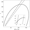 |
Fig. 1 Different segments for the singular point classification (see text for details). The parameters used are Ω = 0.9, α = 1.0, ϵ = 0.1, and η = 0.5. |
3.4 Determining the Range of the Eigenvalues
From Fig. 1, defining  and λ1 as the values of rs/R and λ at the intersection between F = 0 and
  Fu = 0, we obtain
  and λ1 = 129.22. Similarly for the other intersection, we obtain
  and λ2 = 130.82. Using this information we can search for the values of the velocity gradient (w′s±) and the eigenvalue (λ) at the sonic point given by Eq. (27).
Figure 2 shows the value of w′s as a function of the eigenvalue. In order to obtain this value we need to set the value of λ and then evaluate w′s± for the values of  in the range
  for the nodal solution (shown as the black dashed line for w′s+ and the gray dashed line for w′s−). On the other hand, for the saddle solution, we set
  in the range
  . The solid black line shows the branch w′s+ and gray solid line shows the branch w′s−, which is not a physical solution for a transonic decretion disk, because w′s− < 0.
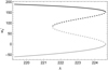 |
Fig. 2 Velocity gradient at the singular point as a function of the eigenvalue λ. The solid lines are for the saddle solutions and the dashed lines for the nodal solutions. The parameters used are the same as in Fig. 1 (see text for details). |
4 Numerical Procedure
Knowing the topology of the nonlinear EoM, we can now describe the numerical procedure to obtain the different viscous transonic decretion disk solutions. Our proposed procedure is the following. First, we define a grid of eigenvalues (λi) in the range (λ1, λ2) for nodal solutions and (aλ1, λ2) for the saddle solution. A typical value of a is 0.7, according our calculations. Second, we integrate from the stellar surface u = −1, with the initial condition w(−1) = 1/λi, up to w(u) = 1 −-ϵ0. When this value of the velocity is attained, the location of the singular point u = us is therefore known. A typical value of ϵ0 is 10−6. Third, for the entire grid of λ; solutions that reached the sonic point, we compare the values of the numerical velocity gradient at the sonic point (w′s)i with the values of w′s− or w′s+, depending on the solution type, obtained from Eq. (27), calculating the absolute error ϕi(λi) = ‖(w′s)i −-w′s±‖. It should be noted that when calculating w′s± from this equation the value of us must lie in the segment of the nodal or saddle solutions depending on the type of solution sought (see Fig. 1). Finally, the eigenvalue λi corresponds to min(ϕi).
Based on this numerical methodology we are now in a condition to perform numerical experiments to understand the behavior of the solutions in terms of the different parameters involved in the EoM.
5 Numerical Calculations
In this section we perform numerical calculations to understand the influence of the different parameters involved in the EoM. All our calculations hereafter are performed for a typical B0 main-sequence star: M = 17.8 M⊙, R = 7.41 R⊙, and Teff = 28 000 K with Tdisk = 0.5 Teff and Ω = 0.9.
5.1 Solutions without Line Force
Following Okazaki (2001), we solve first the EoM without line force, and therefore set η = 0 to describe a pure viscous outflow. Figure 3 shows the normalized velocity profile w(r) as a function of r/R. The eigenvalues are λ = 771.10; 3734.65; 28498.51 for α = 1.0; 0.1; 0.01, respectively. The location of the sonic point is similar for all solutions and lie in the range 425 ≤ rs/R ≤ 479 (see the inset in Fig. 3).
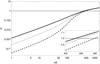 |
Fig. 3 Dimensionless velocity profile (w) for the case without line force (η = 0). The black solid line corresponds to α = 1, the black dotted line is α = 0.1, and the black dashed line is α = 0.01. The inset shows a zoomed-in image of the region around the sonic point. The light gray horizontal solid line represents the sound speed value (w = 1). The stellar parameters are given at the beginning of Sect. 5. |
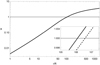 |
Fig. 4 Dimensionless velocity profiles (w) for the two indistinguishable nodal solutions as a function of the r/R coordinate, with α = 1.0 and line-force parameters ϵ = 0.1 and η = 0.5. The inset shows a zoomed-in image of the two solutions around the singular point. The black solid line correspond to the w′s+ branch solution and the dashed line to the w′s− branch solution. The light gray solid line represents the sound speed value (w = 1). The stellar parameters are given at the beginning of Sect. 5. |
5.2 Viscosity Parameter α
Analogously to the results found by Okazaki (2001), the main impact of the viscosity parameter α is the topology of the singular point.
5.2.1 Nodal Solutions
High values of α implies that the sonic point has a nodal topology. This topology shows two branches (dashed lines in Fig. 2). Figure 4 show the velocity profiles for both nodal solutions. The viscosity and line-force parameters are α = 1.0, ϵ = 0.1, η = 0.5, and Tdisk = 0.5 Teff. The two nodal solutions are indistinguishable from each other on the scale of Fig. 4, but in the zoomed-in image around the singular point it is possible to distinguish each one separately. The solution with w′s+ (black solid line) has λ = 223.15 and rs = 107.78 R; the w′s− solution (dashed line) has λ = 222.91 and rs = 106.93 R. For any practical purpose, there is almost no difference in the behavior of the two nodal solutions, and they have almost the same eigenvalue; therefore, we can select either of them.
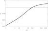 |
Fig. 5 Dimensionless velocity profile (w) (solid black line) for the saddle solution with α = 0.2 and line-force parameters ϵ = 0.1 and η = 0.5. The light gray solid line represents the sound speed value (w = 1). The stellar parameters are given at the beginning of Sect. 5. |
5.2.2 Saddle Solution
Depending on the value of α, the topology switches between saddle and nodal. Using same parameters as the previous nodal case, but with α = 0.2, the resulting saddle solution is shown in Fig. 5. We clearly see here that the location of the sonic point is almost the same as both nodal solutions; here we have λ = 679.63 and rs = 109.62 R.
Although the nodal and saddle solutions, shown in Figs. 4 and 5, only differ in the values of the viscosity parameter α and, consequently, in their topology, the location of the sonic point hardly differs and the velocity profiles w(r) are very similar.
In the next subsections we investigate in detail the role of the different parameters in this viscous transonic decretion outflows.
5.3 Type of Solution Depending on the Value of η
The line-force strength and behavior is determined by the η and ϵ parameters, respectively. Here we study the variation of the η parameter with α = 0.2. Figure 6 shows w(r) for different values of the η parameter with ϵ = 0.1. We confirm that the larger η is, the nearer the sonic point is to the stellar surface. The specific locations are rs/R = 614.8; 109.6; 43.9 for η = 0.1; 0.5; 0.6, respectively. When η = 0.6 the sonic point is located at a distance lower than 50 R, but such a strong force is very unlikely. In Sect. 5.5 we discuss other combinations of line-force parameters and disk temperatures that give similar results about the location of the singular point.
We studied in terms of the α parameter when the solution is nodal or saddle as a function of the η line-force parameter. We find that the switching zone is very narrow, as shown in Fig. 7 and summarized in Table 2.
All the solutions we obtained from the EoM are physical solutions. The characterization of the stability of the steady state can be analyzed by means of the evolution of perturbed waves in the time-dependent equation of motion (see different approaches in Criminale et al. 2018, and references therein), but this type of study is beyond the scope of this work.
5.4 Type of Solution Depending on the Value of Ω
In order to study the influence of the centrifugal force on this viscous disk decretion model, we calculate for different values of Ω the dimensionless velocity profile w as function of r (see Fig. 8). These w(r) profiles show a very unexpected result. They all converge to a unique solution after a very small distance above the stellar surface, r < 1.0004 R, as shown in the inset. Similarly, Fig. 9 shows the behavior of Vϕ(r)/Vcrit as function of r. Again, all solutions converge to a unique solution very near the stellar surface.
A steep gradient in Vϕ(r) might cause a boundary layer, provoking that the specific angular momentum just outside of this layer is settled into a value, which is smoothly connected to the outer parts of the disk. The results shown in Fig. 9 can be used to constrain the value of Ω (or the specific angular momentum) to a much smaller region (i.e., to obtain a smooth solution, in this case Ω ~ 0.7, where the gradients are not steep).
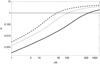 |
Fig. 6 Dimensionless velocity profile w as function of r/R with ϵ = 0.1 and α = 0.2. Here η = 0.1 is shown as a black solid line, η = 0.5 as a black dotted line, and η = 0. 6 as a black dashed line. The light gray solid line represents the sound speed value w = 1 . The stellar parameters are given at the beginning of Sect. 5. |
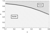 |
Fig. 7 Values of α for nodal and saddle regions as function of η with ϵ = 0.1. The solid black line denotes the lower limit of α for nodal solutions. The light gray line denotes the upper limit of saddle solutions. Hatched zones represents the nodal (upper) and saddle (lower) regions. The stellar parameters are given at the beginning of Sect. 5 (see text for details). |
Topology of the singular points in terms of α and η.
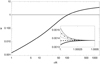 |
Fig. 8 Dimensionless velocity profile, w as function of r/R for different values of Ω with α = 0.2, ϵ = 0.1, and η = 0.5. The gray solid line is Ω = 0.99, the dot-dashed line is Ω = 0.9, the dotted line is Ω = 0.8, the dashed line is Ω = 0.7, and the solid black line is Ω = 0.6. The light gray horizontal line represents the sound speed value, w = 1 . The stellar parameters are given at the beginning of Sect. 5 (see text for details). |
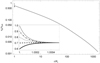 |
Fig. 9 Vϕ(r)/Vcrit as function of r for the same set of parameters a Fig. 8. All solutions converge to one in a very small region above th stellar surface (see text for details). |
Location of the sonic point and its corresponding eigenvalue. in terms of the line-force parameter ϵ with α = 0.2 and η = 0.1.
5.5 Type of Solution Depending on the Line-Force Parameters and Tdisk
We analyze the behavior of the ϵ parameter and the disk temperature Tdisk in the VDD model. The parameter ϵ describes the decay of the line force moving outward from the stellar surface.
Table 3 summarizes the location of the sonic point and eigenvalue in terms of the value of ϵ. The dependence of the line force in terms of r, when Г → 0, is given by (see Eq. (6))
 (31)
(31)
Thus, the larger ϵ is, the slower its decay is in terms of r, and due to a greater line force the location of the sonic point lies closer to the stellar surface.
Table4 summarizes the location of the sonic point and eigen-value in terms of the value of the disk temperature Tdisk and different combinations of line-force parameters η and ϵ. The influence of Tdisk in the location of the sonic point is not determinant when the value of ϵ is high. On the other hand, for low values of ϵ the influence of Tdisk is quite important, reducing the location of rs from ~240R to ~ 160R when Tdisk/Teff increases from 0.5 to 0.9 when η = ϵ = 0.2.
As we pointed out in Sect. 5.3, it is very unlikely to have such a strong line force with η = 0.6. However, it is indeed possible with plausible values of ϵ, η, and Tdisk to obtain transonic disk solutions that might explain the results of Klement et al. (2017).
Location of the sonic point and its corresponding eigenvalue (λ) in terms of the disk temperature Tdisk and line-force parameters ϵ and η.
6 Discussion
In this work we showed the dependence of the velocity field for different parameters involved in the EoM from the VDD model. However, the standard methodology used to obtain an observable, such as Hα, is to use the (volumetric) density (ρ) or the vertical integrated density (Σ) as a function of r/R in a Keplerian orbit as input in radiative transport codes, such as BEDISK (Sigut & Jones 2007) or HDUST (Carciofi & Bjorkman 2006). The standard modeling of ρ is
 (32)
(32)
where ρ(R) = ρ0 is the density at the stellar surface. The definition of Σ follows after integrating ρ(r) in the z direction:
 (33)
(33)
Here2 n = m − 3/2, and Σ(R) = Σ0 is the vertical integrated density at the base of the wind.
Figure 10 shows different values of Σ(r)/Σ(R) as a function of r for the models shown in Sect. 5.3 (see also Fig. 6). The solid gray line represents the fit of Eq. (33) to the vertical integrated density profile for η = 0.6. We clearly see in this figure that none of the solutions maintains the behavior described by Eq. (33) in the entire range of r, but only in the range R < r ≲ 10 R. The results for the fits are n = 0.745 for η = 0.6, n = 0.649 for η = 0.5, and n = 0.554 for η = 0.1. All these values of n are calculated in the interval R ≤ r ≤ 20 R. Fits for the interval R ≤ r ≤ 100 R, give values of n that differ in the fourth decimal place with the previous fit interval. These results shows that the standard formulae giving by ρ(r) or Σ(r) are fairly good approximations to our results, but only for r ≲ 10 R.
A possible explanation for the different behaviors shown in Fig. 10, with different locations of the sonic point for each η (see Sect. 5.3) is the following. Even if the Shakura–Sunyaev viscosity model is applicable to supersonic regions, the viscosity is just as inefficient there as the angular momentum transfer mechanism because the advection timescale in the supersonic region is much shorter than the viscous timescale, which makes the flow to be angular-momentum conserving.
In addition, Klement et al. (2017) studied the observed SED turn-down by means of the VDD model, concluding that it can be explained with a truncated disk. They argued about two possible explanations of this: tidal forces from a close binary companion or a velocity profile with a transonic transition not too far from the star. They assumed that a binary companion is the most probable scenario, but for most of their six sources binarity remained undetected. Nevertheless, we showed in this work, that for a suitable combination of η ϵ, and/or Tdisk it is possible to have singular point locations that explain the SED turn-down without needing a close companion.
In reference to the influence of the stellar rotational speed (in terms of the critical speed) Ω, we found that the viscosity effects collapse all the solutions to (almost) unique w(r) and υϕ(r) profiles in a very small region above the stellar surface, as shown in Figs. 8 and 9. The results from υϕ(r) shown in Fig. 9 can be used to restrict the range of Ω leading to a smooth solution in order to avoid the formation of a boundary layer.
7 Conclusions
We revisited the Okazaki (2001) work of a viscous transonic decretion disk model with the inclusion of a radiative acceleration produced by an ensemble of optically thin lines, described by the Chen & Marlborough (1994) model. We developed a new solution approach, where the eigenvalue of the problem is no longer an angular quantity, but a radial quantity. After a detailed topological analysis of the steady-state equation of motion, three possible physical solutions were found: two nodal solutions, where the viscosity parameter α is larger (nodal region in Fig. 7), and one saddle solution for lower values of α (saddle region in Fig. 7). The two nodal solutions are almost indistinguishable from each other. The value of the viscosity parameter α, given by the Shakura–Sunyaev model, is not determinant for the location of the sonic point. Other parameters, especially those of the line force, η, and ϵ, directly influence the solution of the EoM. Finally, any effect of the stellar rotation is rapidly damped close to the stellar surface due to viscosity. In addition, in order to obtain only smooth solutions the range of Ω should be restricted.
As a future work we will describe the line force using the standard CAK (and its improvements) theory (Castor et al. 1975) instead of the ad hoc model from Chen & Marlborough (1994). With this more detailed model for the line acceleration, it will be possible to incorporate rapid rotational effects such as oblate shape and gravity darkening to better describe a transonic VDD model of Be stars. Finally, to study the observable such as the SED or the line Hα (see Klement et al. 2017) we plan to use the density profile Σ(r) as input in BEDISK and/or HDUST to calculate these observables.
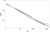 |
Fig. 10 Σ(r)/Σ(R) as function of r with α = 0.2 and ϵ = 0.1 (all stellar parameters are given at the beginning of Sect. 5). Here η = 0.1 is shown as a black solid line, η = 0.5 as a black dotted line, and η = 0.6 as a black dashed line. The light gray line represents the fit of Eq. (33) for the η = 0.6 case (see text for details). |
Acknowledgements
The authors would like to thank the referee, Atsuo Okazaki, for his thoughtful comments and suggestions to improve this work. M.C. and C.A. acknowledge the support from Centro de Astrofísica de Valparaíso. M.C., C.A. and I.A. thank the support from FONDECYT project 1190485. M.C. and C.A. thank to project ANID-FAPESP 2019/13354-1. IA is also grateful for the support from FONDECYT project 11190147. C.A. thanks the support from FONDECYT project 11190945. This project has also received funding from the European Unions Framework Programme for Research and Innovation Horizon 2020 (2014-2020) under the Marie Skłodowska-Curie grant Agreement N° 823734. This work has been possible thanks to the use of AWS-U.Chile-NLHPC credits. Powered@NLHPC: this research was partially supported by the supercomputing infrastructure of the NLHPC (ECM-02).
References
- Amann, H. 1990, Ordinary Differential Equations: An Introduction to Nonlinear Analysis (Berlin: De Gruyter) [CrossRef] [Google Scholar]
- Carciofi, A.C., & Bjorkman, J.E. 2006, ApJ, 639, 1081 [NASA ADS] [CrossRef] [Google Scholar]
- Castor, J.I., Abbott, D.C., & Klein, R.I. 1975, ApJ, 195, 157 [NASA ADS] [CrossRef] [Google Scholar]
- Chen, H., & Marlborough, J.M. 1994, ApJ, 427, 1005 [NASA ADS] [CrossRef] [Google Scholar]
- Criminale, W.O., Jackson, T.L., & Joslin, R.D. 2018, Theory and Computation in Hydrodynamic Stability (Cambridge: Cambridge University Press) [CrossRef] [Google Scholar]
- Curé, M. 2004, ApJ, 614, 929 [CrossRef] [Google Scholar]
- Curé, M., & Rial, D.F. 2004, A&A, 428, 545 [NASA ADS] [CrossRef] [EDP Sciences] [Google Scholar]
- Curé, M., & Rial, D.F. 2007, Astron. Nachr., 328, 513 [CrossRef] [Google Scholar]
- Haubois, X., Carciofi, A.C., Rivinius, T., Okazaki, A.T., & Bjorkman, J.E. 2012, ApJ, 756, 156 [NASA ADS] [CrossRef] [Google Scholar]
- Kee, N.D., & Kuiper, R. 2019, MNRAS, 483, 4893 [NASA ADS] [CrossRef] [Google Scholar]
- Kee, N.D., Owocki, S., & Sundqvist, J.O. 2016, MNRAS, 458, 2323 [NASA ADS] [CrossRef] [Google Scholar]
- Kee, N.D., Owocki, S., & Kuiper, R. 2018a, MNRAS, 474, 847 [NASA ADS] [CrossRef] [Google Scholar]
- Kee, N.D., Owocki, S., & Kuiper, R. 2018b, MNRAS, 479, 4633 [CrossRef] [Google Scholar]
- Klement, R., Carciofi, A.C., Rivinius, T., et al. 2017, A&A, 601, A74 [NASA ADS] [CrossRef] [EDP Sciences] [Google Scholar]
- Krtička, J., Owocki, S.P., & Meynet, G. 2011, A&A, 527, A84 [NASA ADS] [CrossRef] [EDP Sciences] [Google Scholar]
- Kurfürst, P., Feldmeier, A., & Krticka, J. 2014, A&A, 569, A23 [NASA ADS] [CrossRef] [EDP Sciences] [Google Scholar]
- Lee, U., Osaki, Y., & Saio, H. 1991, MNRAS, 250, 432 [Google Scholar]
- Meilland, A., Millour, F., Kanaan, S., et al. 2012, A&A, 538, A110 [CrossRef] [EDP Sciences] [Google Scholar]
- Okazaki, A.T. 2001, PASJ, 53, 119 [NASA ADS] [CrossRef] [Google Scholar]
- Quirrenbach, A., Bjorkman, K.S., Bjorkman, J.E., et al. 1997, ApJ, 479, 477 [NASA ADS] [CrossRef] [Google Scholar]
- Rímulo, L.R., Carciofi, A.C., Vieira, R.G., et al. 2018, MNRAS, 476, 3555 [CrossRef] [Google Scholar]
- Rivinius, T., Carciofi, A.C., & Martayan, C. 2013, A&ARv, 21, 69 [NASA ADS] [CrossRef] [Google Scholar]
- Shakura, N.I., & Sunyaev, R.A. 1973, A&A, 500, 33 [NASA ADS] [Google Scholar]
- Sigut, T.A.A., & Jones, C.E. 2007, ApJ, 668, 481 [NASA ADS] [CrossRef] [Google Scholar]
We use both u and r throughout this work.
For isothermal disks, H(r) ∝ r3/2.
All Tables
Location of the sonic point and its corresponding eigenvalue. in terms of the line-force parameter ϵ with α = 0.2 and η = 0.1.
Location of the sonic point and its corresponding eigenvalue (λ) in terms of the disk temperature Tdisk and line-force parameters ϵ and η.
All Figures
|
Fig. 1 Different segments for the singular point classification (see text for details). The parameters used are Ω = 0.9, α = 1.0, ϵ = 0.1, and η = 0.5. |
| In the text | |
|
Fig. 2 Velocity gradient at the singular point as a function of the eigenvalue λ. The solid lines are for the saddle solutions and the dashed lines for the nodal solutions. The parameters used are the same as in Fig. 1 (see text for details). |
| In the text | |
|
Fig. 3 Dimensionless velocity profile (w) for the case without line force (η = 0). The black solid line corresponds to α = 1, the black dotted line is α = 0.1, and the black dashed line is α = 0.01. The inset shows a zoomed-in image of the region around the sonic point. The light gray horizontal solid line represents the sound speed value (w = 1). The stellar parameters are given at the beginning of Sect. 5. |
| In the text | |
|
Fig. 4 Dimensionless velocity profiles (w) for the two indistinguishable nodal solutions as a function of the r/R coordinate, with α = 1.0 and line-force parameters ϵ = 0.1 and η = 0.5. The inset shows a zoomed-in image of the two solutions around the singular point. The black solid line correspond to the w′s+ branch solution and the dashed line to the w′s− branch solution. The light gray solid line represents the sound speed value (w = 1). The stellar parameters are given at the beginning of Sect. 5. |
| In the text | |
|
Fig. 5 Dimensionless velocity profile (w) (solid black line) for the saddle solution with α = 0.2 and line-force parameters ϵ = 0.1 and η = 0.5. The light gray solid line represents the sound speed value (w = 1). The stellar parameters are given at the beginning of Sect. 5. |
| In the text | |
|
Fig. 6 Dimensionless velocity profile w as function of r/R with ϵ = 0.1 and α = 0.2. Here η = 0.1 is shown as a black solid line, η = 0.5 as a black dotted line, and η = 0. 6 as a black dashed line. The light gray solid line represents the sound speed value w = 1 . The stellar parameters are given at the beginning of Sect. 5. |
| In the text | |
|
Fig. 7 Values of α for nodal and saddle regions as function of η with ϵ = 0.1. The solid black line denotes the lower limit of α for nodal solutions. The light gray line denotes the upper limit of saddle solutions. Hatched zones represents the nodal (upper) and saddle (lower) regions. The stellar parameters are given at the beginning of Sect. 5 (see text for details). |
| In the text | |
|
Fig. 8 Dimensionless velocity profile, w as function of r/R for different values of Ω with α = 0.2, ϵ = 0.1, and η = 0.5. The gray solid line is Ω = 0.99, the dot-dashed line is Ω = 0.9, the dotted line is Ω = 0.8, the dashed line is Ω = 0.7, and the solid black line is Ω = 0.6. The light gray horizontal line represents the sound speed value, w = 1 . The stellar parameters are given at the beginning of Sect. 5 (see text for details). |
| In the text | |
|
Fig. 9 Vϕ(r)/Vcrit as function of r for the same set of parameters a Fig. 8. All solutions converge to one in a very small region above th stellar surface (see text for details). |
| In the text | |
|
Fig. 10 Σ(r)/Σ(R) as function of r with α = 0.2 and ϵ = 0.1 (all stellar parameters are given at the beginning of Sect. 5). Here η = 0.1 is shown as a black solid line, η = 0.5 as a black dotted line, and η = 0.6 as a black dashed line. The light gray line represents the fit of Eq. (33) for the η = 0.6 case (see text for details). |
| In the text | |
Current usage metrics show cumulative count of Article Views (full-text article views including HTML views, PDF and ePub downloads, according to the available data) and Abstracts Views on Vision4Press platform.
Data correspond to usage on the plateform after 2015. The current usage metrics is available 48-96 hours after online publication and is updated daily on week days.
Initial download of the metrics may take a while.