| Issue |
A&A
Volume 679, November 2023
|
|
|---|---|---|
| Article Number | A154 | |
| Number of page(s) | 13 | |
| Section | Extragalactic astronomy | |
| DOI | https://doi.org/10.1051/0004-6361/202346624 | |
| Published online | 30 November 2023 | |
Spiral shocks induced in a galactic gaseous disk: Hydrodynamic understanding of observational properties of spiral galaxies
1
Department of Astronomy, Xiamen University, Xiamen, Fujian 361005, PR China
e-mail: This email address is being protected from spambots. You need JavaScript enabled to view it.
; This email address is being protected from spambots. You need JavaScript enabled to view it.
2
Department of Physics and Institute of Astronomy, National Tsing Hua University, 30013 Hsinchu, Taiwan
Received:
8
April
2023
Accepted:
29
September
2023
Abstract
Context. We investigate the properties of spiral shocks in a steady, adiabatic, non-axisymmetric, self-gravitating, mass-outflowing accretion disk around a compact object.
Aims. We obtained the accretion-ejection solutions in a galactic disk and applied them to spiral galaxies in order to investigate the possible physical connections between some observational quantities of galaxies.
Methods. We considered the self-gravitating disk potential to examine the properties of the galactic gaseous disk. We obtained spiral shock-induced accretion-ejection solutions following the point-wise self-similar approach.
Results. We observed that the self-gravitating disk profoundly affects the dynamics of the spiral structure of the disk and the properties of the spiral shocks. We find that the observational dispersion between the pitch angle and shear rate and between the pitch angle and star formation rate in spiral galaxies contains some important physical information.
Conclusions. There are large differences among the star formation rates of galaxies with similar pitch angles. These differences may be explained by the different star formation efficiencies caused by distinct galactic ambient conditions.
Key words: Galaxy: disk / galaxies: spiral / galaxies: star formation / shock waves
© The Authors 2023
 Open Access article, published by EDP Sciences, under the terms of the Creative Commons Attribution License (https://creativecommons.org/licenses/by/4.0), which permits unrestricted use, distribution, and reproduction in any medium, provided the original work is properly cited.
This article is published in open access under the Subscribe to Open model. This email address is being protected from spambots. You need JavaScript enabled to view it. to support open access publication.
1. Introduction
The existence of spiral structures in accretion disks has long been a topic of interest in both observational and theoretical studies. Observations have provided many pieces of evidence for the existence of a spiral structure in accretion disks (Steeghs et al. 1997; Neustroev & Borisov 1998; Pala et al. 2019; Baptista & Wojcikiewicz 2020; Lee et al. 2020), and there is a general consensus that the spiral shock wave induces a spiral structure in the accretion disk. However, the origin of the shock may correspond to many different mechanisms. In theory, Michel (1984) first proposed the spiral shock in accretion disks as an effective angular momentum transfer mechanism. Sawada et al. (1986a,b) performed two-dimensional hydrodynamic simulations of the Roche lobe overflow in a semi-detached binary system in order to confirm the formation of the spiral shock and the angular momentum transfer in an accretion disk. With the advent of enormous computational facilities, an increasing number of three-dimensional simulations that include the spiral shock have been investigated for the accretion in a binary system (Makita et al. 2000; Molteni et al. 2001; Ju et al. 2016, 2017; Xue et al. 2021).
Though the solution of a numerical simulation is closer to the physical reality, the insight from a simplified model of intrinsic physical laws still plays an essential role in developing an accretion theory. In the theoretical field of study concerning the spiral shock of accretion disks, Spruit (1987) first introduced the radial self-similar simplification for the steady accretion flow in an inertial frame. The same simplification was also adopted in subsequent theoretical studies of accretion disks (e.g., Chakrabarti 1990a; Narayan & Yi 1994). We find it is worth mentioning that a common feature among such studies is the use of the Newtonian gravitational potential, which maintains the mathematical self-consistency of self-similar solutions at different radii. In addition, Narayan & Yi (1994) pointed out that this kind of radial self-similar solution under the Newtonian potential is piece-wise valid, because it can only match the simulations in the middle radial region of accretion disks, where there are fewer effects from the inner and outer boundaries, though they can be applied to all available radii mathematically. Following these theoretical studies, we extended the spiral shock model presented by Spruit (1987) and further improved by Chakrabarti (1990a) from the single star in an inertial frame to the binary system in a non-inertial co-rotating frame and involved the mass outflow induced by spiral shocks as well (Aktar et al. 2021). Accordingly, the Newtonian potential was replaced by the Roche potential as well as the Coriolis force. This allowed us to involve the effects of the binary system on the spiral shock in our model, but our self-similar solution degenerated and became point-wise valid because it was no longer able to keep the separation of variables valid at different radii.
The existence of shock waves in an axisymmetric accretion flow as well as their implication has been extensively studied in the literature both analytically and numerically (Fukue 1987; Chakrabarti 1989; Lu et al. 1999; Becker & Kazanas 2001; Fukumura & Tsuruta 2004; Chakrabarti & Das 2004; Sarkar & Das 2016; Sarkar et al. 2018, 2020; Dihingia et al. 2018, 2019a,b). Due to the shock transition, the post-shock matter becomes very dense and hot, changing into what is known as the post-shock corona (PSC; see Aktar et al. 2015). As a result, a part of the accreting matter is ejected as mass outflow from the disk due to the excess thermal gradient force across the shock. The accretion-ejection process has been widely investigated based on the shock compression model and considering an axisymmetric accretion flow assumption (Chattopadhyay & Das 2007; Das & Chattopadhyay 2008; Kumar & Chattopadhyay 2013; Aktar et al. 2015, 2017, 2019). In the same spirit, Aktar et al. (2021) investigated mass outflow from the disk induced by spiral shock compression in a non-axisymmetric accretion flow.
In another astrophysical field, the spiral structure in galaxies has also been investigated for a long time. The number of spiral arms and the pitch angle (i.e., the angle between the tangent and azimuthal directions on the spiral arm) are both essential criteria of Hubble’s scheme for classifying galaxies (Hubble 1926). Lin & Shu (1964) proposed the famous density wave theory in order to explain the formation and preservation of spiral arms in galaxies. Woodward (1976) performed a two-dimensional hydrodynamical simulation to demonstrate the mechanism of star formation (SF) in the density wave theory. Elmegreen (1979) proposed that the interstellar matter flows through the spiral density wave, becomes shocked, and then collapses due to its self-gravity. Block et al. (1997) studied the spiral arms of M51 and found evidences that the gravitational collapse of the shocked gas triggers the SF in spiral arms.
Inspired by these studies and based on our self-similar model of spiral shocks (Aktar et al. 2021), we were encouraged to investigate the possible correlation between the star formation rate (SFR) and the characteristic quantity of spiral arms, PA, in spiral galaxies. Since the galactic gaseous disk is self-gravitating, our model must be modified to adapt to this new situation (Sect. 2) and involve the SF as a special kind of mass outflow from the gaseous disk (Sect. 4). Additionally, since the self-gravity of a disk depends on the specific disk mass distribution, the self-similar solution of our model would be locally valid point-wise (radius-wise) and would enable us to apply some similar methodologies from our previous work (Aktar et al. 2021).
The paper is organized as follows. In Sect. 2, we present the description of the model and governing equations. In Sect. 3, we discuss the results of our model in detail. In Sect. 4, we apply our model to understand the dispersion between galactic observational quantities. Finally, we draw our conclusions in Sect. 5.
2. Model description
We considered a steady, adiabatic, non-axisymmetric accretion flow around a compact star. We assumed that the effect of gravity on the accretion disk is significant enough compared to the central object. Therefore, we consider a self-gravitating disk in this paper. We also adopted the spiral shock model proposed by Chakrabarti (1990b). In this work, we simultaneously solve the radial and the azimuthal components of momentum equations, and we assume that the accretion flow is in vertical hydrostatic equilibrium throughout the disk.
2.1. Governing equations
In this paper, we write the governing equations in cylindrical coordinates on the equatorial plane. The governing equations are as follows. First is the (i) radial momentum conservation equation,
 (1)
(1)
next is the (ii) azimuthal momentum equation,
 (2)
(2)
third is the (iii) continuity equation,
 (3)
(3)
and finally the (iv) vertical pressure balance equation,
 (4)
(4)
where r, ϕ, vr, vϕ, P, ρ, and 2h are the radial coordinate, azimuthal coordinate, radial component of velocity, azimuthal component of velocity, gas pressure, density of the flow, and local vertical thickness, respectively. The Φ in Eqs. (1) and (4) is the total gravitational potential due to the compact object present at the center of the disk and the self-gravitational potential due to the disk material. The expression of Φ is given in Sect. 2.2. We also use the adiabatic equation of state P = Kργ, where K is the measure of the entropy of the flow. The adiabatic index is expressed as  , and n represents polytropic index of the flow.
2.2. Self-gravitating disk
In an accretion disk, the gravitational field is generally dominated by the central compact object, but in some cases, the disk’s self-gravity can also produce a significant effect. The contribution to the gravitational field due to the disk depends on the matter distribution, and it is obtained by solving Poisson’s equation. For an infinitesimally thin disk, the relation between the surface density of the disk (Σ(r)) and the disk gravitational field (Φd) can be written using the complete elliptic integrals of the first kind (Lodato 2007). The integral form is quite complicated to handle analytically. However, there is a particular simplified relation between Σ and Φd at the disk midplane that was proposed by Mestel (1963). In this work, we consider the gravitational force due to a self-gravitating disk, and it is given by
 (5)
(5)
where Σ = 2ρh is the surface density of the disk. Therefore, the total gravitational force in the presence of a self-gravitating disk as well as the central compact object is given by
 (6)
(6)
where Φc and Φd are the gravitational potentials due to the compact object at the center of the disk and due to the self-gravity of the disk, respectively. Here, G is the gravitational constant. We also introduced a constant factor, σ. When σ = 0, it implies a non-self-gravitating disk (Chakrabarti 1990b), and when σ = 1, it introduces the effect of self-gravity. In this paper, we use the unit system G = M = c = 1 throughout, unless otherwise stated.
We emphasize that in reality, the gravity torque generated by the spiral arm of the spiral galaxy is inevitable (Block et al. 2002, 2004; Tiret & Combes 2008). However, in the present work, we ignore the effect of gravity torque in the presence of the spiral arm in Eq. (6). Further, we mention that the spiral galactic disk is composed of visible and invisible matter, including gaseous matter, stars, and dark matter. In our theoretical model, we assumed the galactic disk is predominately dominated by gaseous matter, and our calculation is independent of mass. However, we do consider the total mass, both visible and invisible, within the radius r when we derive the observational data from the circular velocity curve of spiral galaxies (see Sect. 4). Therefore, our calculation implicitly considers the gravity contribution from the stellar component and the invisible mass.
2.3. Flow equations in spiral coordinates using self-similar conditions
We transformed the conservation equations in cylindrical coordinates to spiral coordinates. The spiral coordinates are defined as ψ = ϕ + β(r). Here, β connects to the radial distances and spirality of the disk. We considered the self-similarity conditions in the spiral coordinate as (Chakrabarti 1990b; Aktar et al. 2021)
 (7a)
(7a)
 (7b)
(7b)
 (7c)
(7c)
 (7d)
(7d)
 (7e)
(7e)
and
 (7f)
(7f)
where, B represents the “spirality” in the flow. The expression of spirality is B = tanθ, where θ represents the pitch angle. The measure of entropy K remains constant along the flow between two consecutive shocks; however, it changes at the shock. In Eq. (7c), a represents the sound speed of the flow. Using the definition of sound speed, we calculate the variation of K as
 (8)
(8)
where,  (Chakrabarti 1990a). The entropy should generally increase inward for accretion and outward for wind. In this paper, we are interested only in the accretion solution. Therefore, we always choose γ < 5/3 to analyze the accretion flow.
We obtained the disk height (h) from Eq. (4) as
 (9)
(9)
where, P = ρa2 and  . Here, α = 4πqρ. It is evident that the disk height is dependent on the density of the material present in the disk for the self-gravitating disk. Here, the surface density of the disk can be obtained as Σ = 2ρh. In general, if the disk is predominately dominated by disk gravity with a negligible central object mass, the surface density follows the Σ ∼ 1/r relation (Bertin & Lodato 1999, 2001). On the other hand, in a real spiral galactic disk, the surface density profile may be completely different, as depicted in Eq. (9). In our model, we consider a point-wise self-similar approach in order to incorporate the spiral coordinate (Aktar et al. 2021). Our self-similarity model is valid point-wise, that is, within a fixed radial distance (r). Therefore, it is difficult to infer the radial dependence of flow variables in the present formalism.
Therefore, we obtained the dimensionless differential equations of q1, q2, and q3 from Eqs. (1)–(4) using Eqs. (7a)–(7f) and (9), and they are given by
 (10)
(10)
 (11)
(11)
and
 (12)
(12)
where, qw = q2 + Bq1.
2.4. Sonic point analysis
We obtained the sonic point conditions by eliminating  and
and  from Eq. (12) using Eqs. (10) and (11), and it is given by
 (13)
(13)
where,
 (14)
(14)
and
 (15)
(15)
During the accretion process into the compact object, the denominator (D) in Eq. (13) becomes zero at some surfaces (known as sonic surface ψ = ψc). Simultaneously, the numerator (N) also has to be zero at sonic surfaces to maintain the smooth solution (Chakrabarti 1989). The vanishing condition of denominator D = 0 provides the sound speed at the sonic surface as
 (16)
(16)
where ![Mathematical equation: $ \Lambda = \left[(\gamma + 1) - \frac{\sigma \alpha r^{-3/2}}{\mathcal{G}^2}\right] $](/articles/aa/full_html/2023/11/aa46624-23/aa46624-23-eq27.gif) .
.
In the presence of shock, the velocity component perpendicular to the shock is
 (17)
(17)
and the velocity component parallel to the shock is given by
 (18)
(18)
The value of the Mach number at the sonic surface is obtained as  using Eqs. (16) and (17). We note that the Mach number at the sonic point deviates from the axisymmetric vertical equilibrium model for the self-gravitating disk.
Also at the sonic surface, the vanishing condition of numerator N = 0 gives rise to the radial velocity (q1c), which is given by
 (19)
(19)
where
![Mathematical equation: $$ \begin{aligned} \mathcal{A}&= - \frac{B^3 (n_\rho + 1)}{(B^2 + 1)} \frac{\Lambda }{2 \gamma } + B - \frac{3}{2}\frac{B r^{-3}}{\mathcal{G} ^2} - \frac{3}{4} \frac{B \sigma \alpha r^{-3/2}}{\mathcal{G} ^2}\nonumber \\ \mathcal{B}&= - \frac{B^2 q_2 (n_\rho +1)}{(B^2 + 1)} \frac{\Lambda }{\gamma } + \frac{B^2 \sigma \alpha }{\mathcal{G} } \left[\frac{\Lambda }{2(B^2 +1)} \right]^{1/2} + 2 q_2\nonumber \\&\quad - \frac{3}{2}\frac{r^{-3}q_2}{\mathcal{G} ^2} - \frac{3}{4} \frac{\sigma \alpha r^{-3/2}q_2}{\mathcal{G} ^2}\nonumber \\ \mathcal{C}&= - \frac{B q_2^2 (n_\rho +1)}{(B^2 + 1)} \frac{\Lambda }{2\gamma } - B q_2^2 + B + \frac{B \sigma \alpha q_2}{\mathcal{G} } \left[\frac{\Lambda }{2(B^2 +1)}\right]^{1/2}, \end{aligned} $$](/articles/aa/full_html/2023/11/aa46624-23/aa46624-23-eq32.gif) (20)
(20)
where the subscript “c” represents the quantities evaluated at the sonic surface. To obtain the derivative  at the sonic surfaces, we applied l’Hospital’s rule in Eq. (13), similar to Aktar et al. (2021).
2.5. Computation of mass outflow rate from the disk
The net mass flux can be obtained from Eq. (3) using self-similar conditions (Eqs. (7a)–(7f)). One part of the mass flux is contributed to the radial inflow mass flux (Ṁin; i.e., accretion rate), and another part is contributed to the wind flux in the azimuthal direction (Chakrabarti 1990b). We find it is notable to mention that Chakrabarti (1990b) did not consider the situation of mass outflow from the disk. In general, if there is no spiral shock in the flow, the wind flux is zero (Chakrabarti 1990b). However, in the presence of spiral shocks, the post-shock matter is very hot and dense. The excess thermal gradient force across shocks drives a part of the accreting matter as a mass outflow in the spiral arm from the disk, similar to the axisymmetric accretion disk model (Aktar et al. 2015, 2017). We mention that we assumed a two-dimensional vertical equilibrium model here (i.e., 2.5D). Therefore, estimating the mass flux component in the vertical direction is impossible in the present model. However, we argue that the mass flux in the azimuthal direction accumulates in the spiral arm and is ejected away as mass outflow from the disk due to the thermal gradient force across spiral shock waves. In our model, if we consider mass outflow, we need to balance non-zero mass flux in the azimuthal direction with mass outflow rates Ṁout in order to maintain the mass conservation Eq. (3).
Therefore, the mass accretion rate in the radial direction can be obtained from Eq. (3) as
 (21)
(21)
The mass outflow rates from the disk were obtained by equating the wind flux normal to the spiral shock in order to preserve the total mass flux in the flow, that is,
 (22)
(22)
Here, the ratio of mass outflow to inflow rates can be calculated as  (Aktar et al. 2015, 2017, 2021).
2.6. Spiral shock conditions and solution methodology
The spiral shock conditions are given by (Chakrabarti 1990b; Aktar et al. 2021). First we present the (1) energy conservation equation:
 (23a)
(23a)
Next we show the (2) momentum conservation equation:
 (23b)
(23b)
Third we present the (3) conservation of mass flux normal to the shock:
 (23c)
(23c)
Last, we show the (4) conservation of velocity component parallel to the flow:
 (23d)
(23d)
where “±” implies post-shock and pre-shock quantities, respectively. Here, W represents the vertically integrated gas pressure of the flow (Matsumoto et al. 1984; Chakrabarti 1989). The shock invariant quantity (Cs) was obtained using Eqs. (23a)–(23c) as
![Mathematical equation: $$ \begin{aligned} C_{\rm s} = \frac{\left[M_{+} (3\gamma -1) + \frac{2}{M_+}\right]}{\left[2 + (\gamma -1)M_{+}^2\right]} = \frac{\left[M_{-} (3\gamma -1) + \frac{2}{M_-}\right]}{\left[2 + (\gamma -1)M_{-}^2\right]}\cdot \end{aligned} $$](/articles/aa/full_html/2023/11/aa46624-23/aa46624-23-eq41.gif) (24)
(24)
We define the shock strength as  . The analytical expression of the shock location ϵ can be obtained from (Chakrabarti 1990b; Aktar et al. 2021), and it is given by
 (25)
(25)
where δψ = 2π/ns, and ns is the number of shocks in the flow. We obtained the calculation of the second-order derivatives at the sonic surfaces in a way similar to that of Aktar et al. (2021). We omitted representing the long expression here in order to avoid repetition. Further, we quantified the amount of specific angular momentum (λ) dissipated in the presence of the spiral shocks as
 (26)
(26)
The classical self-similar solution is a common feature of the Newtonian gravitational potential, and it has been widely investigated in the literature, starting with some pioneering works (Spruit 1987; Chakrabarti 1990b; Narayan & Yi 1994). The self-similar solutions make flow equations dimensionless and independent of position. This approach can be widely applied in various physical situations in accretion physics. However, the classical self-similar approach is unable to incorporate various interesting physical scenarios, such as the non-inertial effects from the co-rotating frame of the binary, the self-gravitating disk, among others. Moreover, the numerical simulations also indicate that the self-similar solution is only valid in the middle radial region of the accretion disk, where there are fewer effects from the inner and outer boundaries (Narayan & Yi 1994). In general, the self-similar solution is only a local solution under local simplification, not a global solution. Recently, Aktar et al. (2021) considered the self-similar condition in order to simplify the two-dimensional calculation and obtain the point-wise valid solution to incorporate the physical effects from the companion gravity, centrifugal force, and Coriolis force. Motivated by this approach, we also adopted the point-wise self-similar solutions in order to investigate spiral shocks in a self-gravitating disk by incorporating the self-gravitating potential in our model.
We adopted the point-wise self-similar approach proposed by Aktar et al. (2021). We first fixed the radial distance (r) of the flow. Then, to obtain the solution, we applied the same input parameters mentioned by Chakrabarti (1990b). Therefore, we supplied the number of shocks (ns), pitch angle (θ), rotational velocity at the sonic surface (q2c), and adiabatic index (γ) of the flow. Additionally, we needed to supply the density (qρc) at the sonic surface due to the consideration of a self-gravitating disk. We self-consistently determined the shock location (ϵ) using Eqs. (24) and (25). We also fixed the adiabatic index to γ = 4/3 throughout the paper, unless otherwise stated.
3. Results
In a non-axisymmetric accretion flow, the inflowing matter spirals around the compact object. During accretion, the flow might encounter several spiral shock transitions, depending on the flow parameters (Chakrabarti 1990b; Aktar et al. 2021). Due to the shock transition, the flow loses its angular momentum (see Eq. (26)) and enters into the central compact object. If the gravitational field due to the matter present in the disk is significant enough, the self-gravitating effect needs to be incorporated in governing equations. Keeping this in mind, we considered the self-gravitating effect in our present formalism. To obtain the solutions, we first needed to examine the nature of the sonic surfaces, which can be determined following the quadratic expression of  at the sonic surfaces. The sonic surfaces can be broadly classified as either being physical (discriminant > 0) or unphysical (discriminant < 0). The physical sonic surfaces are also classified as being “saddle type”, “straight line”, or “nodal type”, depending on various conditions (see Aktar et al. 2021; Chakrabarti 1990a for details). In this work, we first identified the saddle-type sonic surfaces by supplying the inflow parameters, namely, the pitch angle (θ), the rotational velocity at the sonic surface (q2c), and the density of matter (qρc) at the radial position (r) (Chakrabarti 1989, 1990b). To obtain solutions, we numerically integrated Eqs. (10)–(12) from saddle-type sonic surfaces by supplying the flow variables (θ, q2c, qρc, γ) and using both the positive or negative slopes of
  , at a particular radial distance r (see Aktar et al. 2021). During accretion, the flow passes through spiral shocks, and due to the shock compression, a part of the accreting matter emerges from the disk as mass outflows (Aktar et al. 2015, 2017, 2021). We calculated the mass outflow rates using Eqs. (21) and (22). To begin, we first investigated the difference between non-self-gravitating and self-gravitating disk accretion flows. For the purpose of the comparison, we investigated the Mach number (M), rotational velocity (q2), sound speed (
 ), and density of the matter (qρ) with the spiral coordinates. In panel a of Fig. 1, we compare the Mach number with spiral coordinates (ψ). We observed that the Mach number variation is completely different for the self-gravitating disk compared to the non-self-gravitating disk. Moreover, the Mach number at the sonic point (Mc) is different from the non-self-gravitating disk, as indicated in Eqs. (16) and (17) and depicted in Fig. 1a. In a similar manner, the rotational velocity (q2) and the sound speed or equivalent disk height (
 ) varies significantly in the presence of a self-gravitating disk, as shown in Figs. 1b and c, respectively. The disk height clearly increases in a particular radial position with the spiral coordinates for a self-gravitating disk compared to a non-self-gravitating disk, depicted in Fig. 1c. However, we also observed that the density of matter (qρ) also deviates from the non-self-gravitating disk, even when starting from the same sonic values, as shown in Fig. 1d. In Fig. 1, we fixed the flow parameters (θ, q2c, qρc) as (50° ,0.10, 10−4) at the radial distance r = 25. The solid red curve represents a self-gravitating disk, and the dashed black curve represents a non-self-gravitating disk. The saddle-type sonic surfaces (ψc) are indicated in the figure. We note that the particular solution mentioned in Fig. 1 does not exhibit spiral shocks.
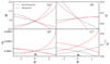 |
Fig. 1. Comparison of flow variables for a non-self-gravitating disk and a self-gravitating disk with the spiral coordinates. The panels a–d present the Mach number (M), rotational velocity (q2), sound speed or equivalent disk height ( |

We also compared the solution topology between non-self-gravitating and self-gravitating disks (Fig. 2) for ns = 2. During accretion, the inflowing matter passes through some sonic surfaces (ψc) in order to become supersonic. If the spiral shock conditions (Eqs. (23a)–(25)) are satisfied, then the flow makes a discontinuous jump to the subsonic flow. Immediately, the flow increases velocity and passes through another sonic surface. Again, the shock transition happens, and the flow loses its angular momentum. Finally, the matter enters into the compact object. In Fig. 2, the vertical arrows indicate the spiral shock transitions in the flow, and the solid (black) circles represent sonic surfaces. In this figure, the solid red and dashed black lines respectively represent a self-gravitating and a non-self-gravitating disk. Notably, we found two spiral shocks (ns = 2) for the self-gravitating disk, though there are no spiral shocks present in the non-self-gravitating flow for the same inflow parameters. The corresponding sonic surfaces (ψ1c, ψ2c, ψ3c) and shock locations (ψs1, ψs2) are also indicated in the figure. In this case, the shock parameters are (ϵ, 𝒮) = (0.2700, 1.9526). In a similar way, we also present the solution topology in the presence of a self-gravitating disk when the number of spiral shocks is ns = 4, depicted in Fig. 3. The corresponding four sonic surfaces (ψ1c, ψ2c, ψ3c) and four shock locations (ψs1, ψs2, ψs3, ψs4) are shown in the figure. The corresponding shock parameters are (ϵ, 𝒮) = (0.3469, 2.7238). We fixed the flow parameters (θ, q2c, qρc, r) as (60° ,0.86, 10−4, 25) for Fig. 2 and as (45° ,0.75, 10−5, 20) for Fig. 3.
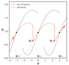 |
Fig. 2. Comparison of solution topology for a non-self-gravitating disk and a self-gravitating disk. The flow variables are (θ, q2c, qρc) = (60° ,0.86, 10−4). We also fixed the radial distance at r = 25. See the text for details. |
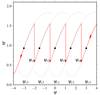 |
Fig. 3. Representation of the spiral shock transitions for the number of shocks ns = 4 in the presence of a self-gravitating disk. The vertical arrows represent the spiral shock transitions in the flow. The flow parameters are (θ, q2c, qρc, r) = (45° ,0.75, 10−5, 20). See the text for details. |
We examined the overall behavior of shock properties in terms of pitch angle by fixing all other flow parameters. In Fig. 4a, we represent the shock location (ϵ) with the variation of pitch angle (θ). The solid black, dashed red, dotted blue, and dashed-dotted green lines are for different flow densities at the sonic surface, namely, qρc = 0.0001, 0.1, 0.2, and 0.3. The corresponding shock strength (𝒮) is plotted in Fig. 4b. We observed that shock strength decreases with the increase of pitch angle. This implies that a tighter spiral arm exhibits stronger spiral shocks in the flow. Also, shock strength decreases with the increase of density of the flow for a particular pitch angle. Similar trends have been observed for the dissipation of angular momentum (Δλ), depicted in Fig. 4c. We plotted the mass outflow rates (Rṁ) in Fig. 4d and found that the mass outflow rates increase with the pitch angle. This clearly indicates that spiral shocks cause gaseous matter to escape more easily from the disk in a weakly wound spiral arm compared to one that is more tightly wound. Also, mass outflow rates are higher for a denser flow than a less dense flow for a particular pitch angle due to the availability of more matter in the disk surface. In Fig. 4, we fixed the rotational velocity q2c = 0.6 at the radial distance r = 0.01.
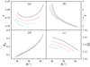 |
Fig. 4. Variation of (a) shock locations (ϵ); (b) shock strength (𝒮); (c) amount of angular momentum dissipation (Δλ) across shock; and (d) mass outflow rate (Rṁ) in terms of the pitch angle for various flow densities at the sonic surface (qρc). The solid (black), dashed (red), dotted (blue), and dashed-dotted (green) lines are for qρ = 0.0001, 0.1, 0.2, and 0.3, respectively. We fixed q2c = 0.60 at the radial distance r = 0.01. See the text for details. |
After comparing the solution topology, we then investigated the overall parameter space containing spiral shocks. The shock parameter space is separated by pitch angle (θ) and rotational velocity (q2c) at sonic surfaces, as shown in Fig. 5. Theoretically, the number of spiral shocks lies within the range 1 ≥ ns → ∞ (Spruit 1987). Therefore, we compared the parameter space for a self-gravitating disk for the number of shocks ns = 2, 4, and 10. We fixed the radial distance at r = 10 and the density at the sonic surface to qρc = 10−4. We observed that the shock parameter space increases significantly from ns = 2 to ns = 4 and then decreases again for ns = 10. There is a clear indication that the parameter space shrinks when there is a greater number of shocks ns. This also indicates that the shock solutions are less probable for a greater number of shock solutions. We also plotted the parameter space for a non-self-gravitating disk, which is independent of radial position (Chakrabarti 1990b). In this case, we chose the number of shocks to be ns = 4. In Fig. 5, the solid black, dotted red, and dashed blue lines are for self-gravitating disks with the number of shocks being ns = 2, 4, and 10, respectively. The remaining dashed-dotted green curve is for the non-self-gravitating disk. The parameter space of the non-self-gravitating disk is the same as in Fig. 6 of Chakrabarti (1990b) for the accretion solution (i.e., σ = 0).
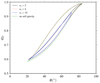 |
Fig. 5. Parameter space for different numbers of spiral shocks (ns). We fixed the radial distance at r = 10 and the flow density as qρc = 10−4. See the text for details. |
4. Application to spiral galactic gaseous disks
In this section, we apply our model to spiral galactic gaseous disks. The shock compression due to spiral shocks drives some of the shocked gaseous matter to form a star, while some of the matter directly outflow from the galactic disk. The detailed physical processes of SF nonetheless depend on the specific galactic environment. In our present work, inferring the galactic environment and the various other physical processes is impossible. Two parameters, namely, PA and shear rate (SR), play pivotal roles in spiral galaxy properties. We assumed that the spiral shock wave and the spiral arm have the same PA since they are always associative; however, they are actually a little different. Therefore, in this section, we consider the PA estimated by the galaxy image analysis as the PA of the spiral shock wave. For the SR (Γ), its definition can easily be found in previous works (e.g., Seigar et al. 2005, 2006; Yu & Ho 2019) and is given as
 (27)
(27)
where r and Vc are the radial distance and the circular velocity around the galactic center, respectively. In our model, the azimuthal velocity vϕ is identical to the Vc in Eq. (27). Therefore, by replacing Vc with Eq. (7b) and doing the mathematical simplification, we obtain from Eq. (27)
 (28)
(28)
where k ≡ dlnq2/dψ, which is one of the derivatives in our model (see Eq. (11)) and represents the changing rate of azimuthal velocity along the ψ-direction. It is an interesting fact that Γ is equal to 3/2 if the Keplerian velocity  is substituted into Eq. (27), which implies the effect of the mass M is only concentrated inside the radius r (not mass outside r). Therefore, on the right side of Eq. (28), 3/2 is the Keplerian upper limit of SR, and the term of ktanθ represents the effects from the disk mass and dark matter halo.
The PA, θ, can be measured from galaxy images through the discrete Fourier transformation, and the SR, Γ, can be estimated by fitting the circular velocity curve (CVC) of the galaxy. Seigar et al. (2005, 2006) supplied a set of PAs and SRs for a total of 45 galaxies based on images in the near-infrared or optical band and the observational CVCs, respectively. Recently, Yu & Ho (2019) also provided a new data set including 79 galaxies, whose PAs were measured from their optical images in the Sloan Digital Sky Survey (SDSS), and SRs came from Kalinova et al. (2017), who used the CVCs of the Calar Alto Legacy Integral Field Area (CALIFA).
In Fig. 6, we present a plot of θ versus Γ, which contains the contours of k defined in Eq. (28) and the data points of 124 galaxies collected from Seigar et al. (2005, 2006), green triangles, and Yu & Ho (2019), blue circles. As can be clearly seen, most of the data points (green and blue) are distributed in the area between two lines of k = 0.5 and 5.0, and the dispersion of PA gradually contracts along the contour lines of k as the SR increases and approaches the limit of 3/2. This interesting contractivity shows the intrinsic physical properties of this dispersion, which can be measured by k with Eq. (28). We can calculate k from the observational PA and SR on a specific galaxy case and fix the derivate dlnq2/dψ in our model in order to constrain the property of spiral shocks coherent to spiral arms in this galaxy.
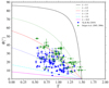 |
Fig. 6. Theoretical value of k in terms of pitch angle and shear rate. The blue circles and green triangles respectively represent the observational data of Yu & Ho (2019) and Seigar et al. (2005, 2006). See the text for details. |
Encouraged by this estimation of the theoretical value of k, we continued to analyze the correlations between the SFR and PA. In order to achieve this goal, we first needed to calculate the physical quantities in a proper unit system. Hereafter, we use the unit system of G = VK = r = 1 instead of G = M = c = 1, which was used in the earlier part of this paper. In this unit system,  is the Keplerian velocity at location r, and the mass M includes all of the visible and invisible mass, such as the gas, dust, star, and dark matter, inside the radius r. In order to estimate VK for a particular galaxy, we assumed that the stars are approximately rotating with the local Keplerian velocity (we note that the vϕ in our model is the circular velocity of the gas; because our model is a hydrodynamic model, vϕ is not necessarily Keplerian and is scaled with the local Keplerian velocity). Then, we could obtain the local star rotating velocity at the location r by interpolation from the CVC of this galaxy. Based on the principal component analysis (PCA) of Kalinova et al. (2017), we could obtain this physical quantity accurately and conveniently through their PCA interpolating formulas. As mentioned earlier, our model solution is point-wise valid, and our analysis is restrained locally. Therefore, the location r refers to the radial distance from the galaxy’s center to where these analyses and measurements occur. In this regard, we estimated r as the radius of the middle point of the range used by Fourier analysis for the PA (i.e., r = rmid), which is the most probable measuring location of PA. Yu & Ho (2019) provided the radial ranges in units of arcseconds for their 79 galaxies, and we obtained the distances from Earth to these galaxies in units of megaparsecs from the data set of CALIFA so we could ultimately calculate the rmid in units of parsecs, which are listed in Table A.1 (Col. 6) for every galaxy from Yu & Ho (2019). Moreover, we needed to fix the number of spiral shocks ns for our model. Thus, we assumed the Fourier mode used to calculate the pitch angle in Yu & Ho (2019) as the number of shocks (see Col. 4 of Table A.1). Unfortunately, we did not find any observational distance for the 45 galaxies analyzed by Seigar et al. (2005, 2006), so we could not continue to use their sample in the subsequent analysis of this paper.
Next, we continued to estimate the SFR based on our model. As mentioned in the Sect. 2.5, we can calculate the outflow rate (Eq. (22)), which is regarded as the estimation of SFR induced by spiral shocks (arms) in our model. However, we were still unable to determine this SFR for each specific galaxy because there are two undetermined parameters (q2c and qρc). These two parameters represent the circular velocity and density of flow at the sonic surface, and their values might depend on the galactic ambient conditions at the shock front, but they cannot be estimated through the existing observational data in this paper. We can only explore the parameter space by varying these two parameters (q2c, qρc) when determining the SFR range for each specific galaxy. In Fig. 7, we show the plot of SFR versus PA. With the SFRs from Catalán-Torrecilla et al. (2015), 79 data points for galaxies of Yu & Ho (2019) are included with their error bars. The area between the black solid (upper limit) and dotted (lower limit) lines denote the SFR range estimated by our model, and most of the data points are within this area, except for several points above the upper limit at the low PA part. The solid lines were produced by connecting the maximum SFR estimation for all individual galaxies for different SFEs, and the dotted line is for the minimum SFRs for SFE = 100%, shown in Fig. 7. The scattered points of observational SFRs show that the parameter space composed of q2c and qρc can reasonably explain the dispersion among the data points (i.e., the differences in galactic ambient conditions cause the differences in SFRs). This in turn shows the rationality of our model. The trend of a rising SFR with an increasing PA is shown in both the upper (solid lines) and lower limit (dotted lines) and is a rational theoretical relationship predicted by our model. However, it is difficult for the trend to be reflected in the dispersive observed SFR data points. A subsequent analysis of our model revealed the reason for this deviation between the theory and the observation. The observed pitch angle (θ), shear rate (Γ), number of shocks (ns), local Keplerian velocity (VK), and mid radial distance of the disk (rmid) are shown in Table A.1. The other theoretical model parameters, such as k, q2c, and qρc, are tabulated in Cols. 7–9 of Table A.1. We also report the corresponding pre-shock (q2−) and post-shock (q2+) rotational velocity in Cols. 10 and 11, respectively. We found that due to the SF, the post-shock velocity is always lower compared to the pre-shock velocity for all the cases. This implies that gas loses its angular momentum allowing it to shift toward lower angular momentum orbits and settles down after SF (see Eq. (26)). The maximum and minimum SFRs are shown in Col. 12 of Table A.1 for a star formation efficiency (SFE) of 100%. We also tabulated the available observed SFRs (SFRobs) for spiral galaxies from Catalán-Torrecilla et al. (2015) in Col. 13 of Table A.1.
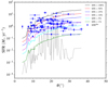 |
Fig. 7. Model-calculated maximum and minimum SFRs in terms of pitch angle (θ) for 79 spiral galaxies. The solid and dotted black lines indicate the maximum and minimum of theoretically estimated SFRs at SFE = 100%. The colored solid lines are the maximum SFRs at different SFEs. The solid blue circles represent the observed SFRs (SFRObs) (Catalán-Torrecilla et al. 2015). See the text for details. |
Through further analysis, we obtained more physical insights from Fig. 7. The dynamics of the outflow gas from the galaxy’s gaseous disk are not included in our model, so we have no way of knowing how the gas left, but there are only two possibilities. One is the disk wind, and the other is SF. Unfortunately, we cannot determine or constrain the individual fractions of disk wind or SF on the total outflow through the observational data in this paper. In fact, it is equivalent to assuming 100% of the compressed outflow gas forms stars that the outflow rate calculated with Eq. (22) is directly regarded as SFR. Obviously, it is impossible to achieve an SFE of 100% in reality. Thus, we also drew a series of upper limits under different SFEs in Fig. 7 (see colored lines parallel to the black line). These lines show the differences in SFEs among these galaxies, which may be caused by the galactic ambient conditions manifested by parameters q2c and qρc in our model. We speculate that compared with the SFR induced by spiral arms, those galaxies close to the 1% limit might have large disk wind launched from arms, while those beyond the 100% limit (even including those beyond 50%) might have other, stronger SF mechanisms. These speculations need further observations and simulations to be confirmed, but it is beyond the scope of our study in this paper.
5. Discussion and conclusions
In this paper, we assumed a non-axisymmetric, inviscid, self-gravitating accretion flow around a compact object. We calculated the spiral shocks in the flow following the prescription of Chakrabarti (1990b). We also adopted the same solution methodology, that is, a point-wise self-similar approach, based on our earlier work (Aktar et al. 2021). In general, the matter distribution in the disk should be considered via Poisson’s equation. However, it is challenging to handle analytically in order to get the self-gravitating effect. As a result, we considered a simplified relation between disk surface density and gravitational potential due to self-gravity (Mestel 1963; Lodato 2007). Our self-gravitating model immediately reduces to the model of Chakrabarti (1990b) in the absence of self-gravity, that is, when σ = 0 (see Eq. (6)). We compared the flow variables of accretion in terms of spiral coordinates for non-self-gravitating and self-gravitating disks, shown in Fig. 1. We observed that the evolution of flow variables is completely different in the presence of self-gravitating disks. In the same spirit, we compared the solution topology, Fig. 2. We found that the flow exhibits spiral shocks for self-gravitating disks even though there is no shock for non-self-gravitating disks for the same set of flow parameters. We also observed that two-shock and four-shock solutions are possible in the presence of self-gravitating disks (see Figs. 2 and 3). Moreover, we observed that mass outflow rates increase with the increase of pitch angle, which indicates that in a weakly wound spiral arm, gaseous mass can easily escape from the disk due to spiral shocks, as depicted in Fig. 4.
Further, we compared and examined the overall shock parameter space separated by pitch angle (θ) and rotational velocity at the sonic surface (q2c) by varying the number of shocks (ns). We observed that the shock parameter space shrinks with an increasing number of shocks, shown in Fig. 5. Finally, we attempted to calculate the SFR of 79 spiral galaxies based on our accretion-ejection model. Interestingly, we observed that the mass outflow triggered by spiral shock waves serves as one of the essential physical mechanisms for the SFR, depicted in Fig. 7. Moreover, our model-calculated SFR is consistent with the observed SFR for various spiral galaxies.
Looking back at the analysis of the PA-SR and SFR-PA correlation depicted in Figs. 6 and 7, which are both shown as very dispersive relationships by observational data, we concluded that the dispersion of data also contains rich physical information, which needs to be extracted by appropriate theoretical models, and ours is just a simple attempt in this regard. We also admit that the physical mechanism of the SFR is extremely complex. There are various other mechanisms (such as active galactic nuclei feedback, supernova, etc.) that may trigger the SFR in a galaxy (Salomé et al. 2016; Padoan et al. 2017; Mukherjee et al. 2018; Cosentino et al. 2022).
In this work, we avoided any dissipation mechanisms in the disk. However, in a realistic situation, various types of dissipation are present in the flow. In a complete scenario, we would need to incorporate the viscous effect along with various cooling mechanisms to get the complete picture, and it would change the flow dynamics (Chakrabarti & Das 2004; Aktar et al. 2017). Moreover, as already pointed out, the dynamics of spiral shocks become significantly affected in the presence of radiative losses in the disk (Spruit 1987). Also, the radiative processes are very significant in galactic disks. The present work investigated the spiral shock properties in radiatively inefficient galactic disks (i.e., in an adiabatic condition). Further, the gravitational instabilities redistribute the angular momentum in the disk (Binney & Tremaine 1987; Bertin & Lodato 1999). Further, we did not consider the gravity torque effect in our model, which is essential in a spiral galactic disk (Block et al. 2002, 2004; Tiret & Combes 2008). Moreover, one of the major limitations of the point-wise self-similar approach is that it is impossible to investigate the global radial variations of flow variables. To analyze this more rigorously, we would need a time-dependent simulation study. This kind of study is beyond our scope in the present formalism. We hope to address these issues in the future.
Acknowledgments
We thank the anonymous referee for very useful comments and suggestions that improved the quality of the paper. The authors also want to express their humble gratitude to Si-Yue Yu for various fruitful discussions during the preparation of the manuscript. The work was supported by the Natural Science Foundation of Fujian Province of China (No. 2023J01008).
References
- Aktar, R., Das, S., & Nandi, A. 2015, MNRAS, 453, 3414 [Google Scholar]
- Aktar, R., Das, S., Nandi, A., & Sreehari, H. 2017, MNRAS, 471, 4806 [NASA ADS] [CrossRef] [Google Scholar]
- Aktar, R., Nandi, A., & Das, S. 2019, Ap&SS, 364, 22 [NASA ADS] [CrossRef] [Google Scholar]
- Aktar, R., Xue, L., & Liu, T. 2021, ApJ, 922, 120 [NASA ADS] [CrossRef] [Google Scholar]
- Baptista, R., & Wojcikiewicz, E. 2020, MNRAS, 492, 1154 [CrossRef] [Google Scholar]
- Becker, P. A., & Kazanas, D. 2001, ApJ, 546, 429 [CrossRef] [Google Scholar]
- Bertin, G., & Lodato, G. 1999, A&A, 350, 694 [NASA ADS] [Google Scholar]
- Bertin, G., & Lodato, G. 2001, A&A, 370, 342 [NASA ADS] [CrossRef] [EDP Sciences] [Google Scholar]
- Binney, J., & Tremaine, S. 1987, Galactic Dynamics (Princeton: Princeton University Press) [Google Scholar]
- Block, D. L., Elmegreen, B. G., Stockton, A., & Sauvage, M. 1997, ApJ, 486, L95 [NASA ADS] [CrossRef] [Google Scholar]
- Block, D. L., Bournaud, F., Combes, F., Puerari, I., & Buta, R. 2002, A&A, 394, L35 [NASA ADS] [CrossRef] [EDP Sciences] [Google Scholar]
- Block, D. L., Buta, R., Knapen, J. H., et al. 2004, AJ, 128, 183 [NASA ADS] [CrossRef] [Google Scholar]
- Catalán-Torrecilla, C., Gil de Paz, A., Castillo-Morales, A., et al. 2015, A&A, 584, A87 [NASA ADS] [CrossRef] [EDP Sciences] [Google Scholar]
- Chakrabarti, S. K. 1989, ApJ, 347, 365 [NASA ADS] [CrossRef] [Google Scholar]
- Chakrabarti, S. K. 1990a, Theory of Transonic Astrophysical Flows (World Scientific Publishing Co.) [CrossRef] [Google Scholar]
- Chakrabarti, S. K. 1990b, ApJ, 362, 406 [NASA ADS] [CrossRef] [Google Scholar]
- Chakrabarti, S. K., & Das, S. 2004, MNRAS, 349, 649 [NASA ADS] [CrossRef] [Google Scholar]
- Chattopadhyay, I., & Das, S. 2007, New Astron., 12, 454 [NASA ADS] [CrossRef] [Google Scholar]
- Cosentino, G., Jiménez-Serra, I., Tan, J. C., et al. 2022, MNRAS, 511, 953 [NASA ADS] [CrossRef] [Google Scholar]
- Das, S., & Chattopadhyay, I. 2008, New Astron., 13, 549 [NASA ADS] [CrossRef] [Google Scholar]
- Dihingia, I. K., Das, S., & Mandal, S. 2018, MNRAS, 475, 2164 [NASA ADS] [CrossRef] [Google Scholar]
- Dihingia, I. K., Das, S., & Nandi, A. 2019a, MNRAS, 484, 3209 [NASA ADS] [CrossRef] [Google Scholar]
- Dihingia, I. K., Das, S., Maity, D., & Nandi, A. 2019b, MNRAS, 488, 2412 [CrossRef] [Google Scholar]
- Elmegreen, B. G. 1979, ApJ, 231, 372 [NASA ADS] [CrossRef] [Google Scholar]
- Fukue, J. 1987, PASJ, 39, 309 [NASA ADS] [Google Scholar]
- Fukumura, K., & Tsuruta, S. 2004, ApJ, 611, 964 [NASA ADS] [CrossRef] [Google Scholar]
- Hubble, E. P. 1926, ApJ, 64, 321 [Google Scholar]
- Ju, W., Stone, J. M., & Zhu, Z. 2016, ApJ, 823, 81 [NASA ADS] [CrossRef] [Google Scholar]
- Ju, W., Stone, J. M., & Zhu, Z. 2017, ApJ, 841, 29 [NASA ADS] [CrossRef] [Google Scholar]
- Kalinova, V., Colombo, D., Rosolowsky, E., et al. 2017, MNRAS, 469, 2539 [Google Scholar]
- Kumar, R., & Chattopadhyay, I. 2013, MNRAS, 430, 386 [NASA ADS] [CrossRef] [Google Scholar]
- Lee, C.-F., Li, Z.-Y., & Turner, N. J. 2020, Nat. Astron., 4, 142 [CrossRef] [Google Scholar]
- Lin, C. C., & Shu, F. H. 1964, ApJ, 140, 646 [Google Scholar]
- Lodato, G. 2007, Nuovo Cimento Rivista Serie, 30, 293 [NASA ADS] [Google Scholar]
- Lu, J.-F., Gu, W.-M., & Yuan, F. 1999, ApJ, 523, 340 [NASA ADS] [CrossRef] [Google Scholar]
- Makita, M., Miyawaki, K., & Matsuda, T. 2000, MNRAS, 316, 906 [NASA ADS] [CrossRef] [Google Scholar]
- Matsumoto, R., Kato, S., Fukue, J., & Okazaki, A. T. 1984, PASJ, 36, 71 [NASA ADS] [Google Scholar]
- Mestel, L. 1963, MNRAS, 126, 553 [NASA ADS] [CrossRef] [Google Scholar]
- Michel, F. C. 1984, ApJ, 279, 807 [CrossRef] [Google Scholar]
- Molteni, D., Kuznetsov, O. A., Bisikalo, D. V., & Boyarchuk, A. A. 2001, MNRAS, 327, 1103 [CrossRef] [Google Scholar]
- Mukherjee, D., Bicknell, G. V., Wagner, A. Y., Sutherland, R. S., & Silk, J. 2018, MNRAS, 479, 5544 [NASA ADS] [CrossRef] [Google Scholar]
- Narayan, R., & Yi, I. 1994, ApJ, 428, L13 [Google Scholar]
- Neustroev, V. V., & Borisov, N. V. 1998, A&A, 336, L73 [NASA ADS] [Google Scholar]
- Padoan, P., Haugbølle, T., Nordlund, Å., & Frimann, S. 2017, ApJ, 840, 48 [Google Scholar]
- Pala, A. F., Gänsicke, B. T., Marsh, T. R., et al. 2019, MNRAS, 483, 1080 [NASA ADS] [CrossRef] [Google Scholar]
- Salomé, Q., Salomé, P., Combes, F., Hamer, S., & Heywood, I. 2016, A&A, 586, A45 [NASA ADS] [CrossRef] [EDP Sciences] [Google Scholar]
- Sarkar, B., & Das, S. 2016, MNRAS, 461, 190 [NASA ADS] [CrossRef] [Google Scholar]
- Sarkar, B., Das, S., & Mandal, S. 2018, MNRAS, 473, 2415 [NASA ADS] [CrossRef] [Google Scholar]
- Sarkar, S., Chattopadhyay, I., & Laurent, P. 2020, A&A, 642, A209 [NASA ADS] [CrossRef] [EDP Sciences] [Google Scholar]
- Sawada, K., Matsuda, T., & Hachisu, I. 1986a, MNRAS, 219, 75 [NASA ADS] [Google Scholar]
- Sawada, K., Matsuda, T., & Hachisu, I. 1986b, MNRAS, 221, 679 [NASA ADS] [CrossRef] [Google Scholar]
- Seigar, M. S., Block, D. L., Puerari, I., Chorney, N. E., & James, P. A. 2005, MNRAS, 359, 1065 [CrossRef] [Google Scholar]
- Seigar, M. S., Bullock, J. S., Barth, A. J., & Ho, L. C. 2006, ApJ, 645, 1012 [NASA ADS] [CrossRef] [Google Scholar]
- Spruit, H. C. 1987, A&A, 184, 173 [NASA ADS] [Google Scholar]
- Steeghs, D., Harlaftis, E. T., & Horne, K. 1997, MNRAS, 290, L28 [Google Scholar]
- Tiret, O., & Combes, F. 2008, A&A, 483, 719 [NASA ADS] [CrossRef] [EDP Sciences] [Google Scholar]
- Woodward, P. R. 1976, ApJ, 207, 484 [NASA ADS] [CrossRef] [Google Scholar]
- Xue, L., Jiao, C.-L., & Li, Y. 2021, MNRAS, 501, 664 [Google Scholar]
- Yu, S.-Y., & Ho, L. C. 2019, ApJ, 871, 194 [NASA ADS] [CrossRef] [Google Scholar]
Appendix A: Spiral galaxy and their star formation rate
Parameters for spiral galaxy.
All Tables
All Figures
|
Fig. 1. Comparison of flow variables for a non-self-gravitating disk and a self-gravitating disk with the spiral coordinates. The panels a–d present the Mach number (M), rotational velocity (q2), sound speed or equivalent disk height ( |
| In the text | |
|
Fig. 2. Comparison of solution topology for a non-self-gravitating disk and a self-gravitating disk. The flow variables are (θ, q2c, qρc) = (60° ,0.86, 10−4). We also fixed the radial distance at r = 25. See the text for details. |
| In the text | |
|
Fig. 3. Representation of the spiral shock transitions for the number of shocks ns = 4 in the presence of a self-gravitating disk. The vertical arrows represent the spiral shock transitions in the flow. The flow parameters are (θ, q2c, qρc, r) = (45° ,0.75, 10−5, 20). See the text for details. |
| In the text | |
|
Fig. 4. Variation of (a) shock locations (ϵ); (b) shock strength (𝒮); (c) amount of angular momentum dissipation (Δλ) across shock; and (d) mass outflow rate (Rṁ) in terms of the pitch angle for various flow densities at the sonic surface (qρc). The solid (black), dashed (red), dotted (blue), and dashed-dotted (green) lines are for qρ = 0.0001, 0.1, 0.2, and 0.3, respectively. We fixed q2c = 0.60 at the radial distance r = 0.01. See the text for details. |
| In the text | |
|
Fig. 5. Parameter space for different numbers of spiral shocks (ns). We fixed the radial distance at r = 10 and the flow density as qρc = 10−4. See the text for details. |
| In the text | |
|
Fig. 6. Theoretical value of k in terms of pitch angle and shear rate. The blue circles and green triangles respectively represent the observational data of Yu & Ho (2019) and Seigar et al. (2005, 2006). See the text for details. |
| In the text | |
|
Fig. 7. Model-calculated maximum and minimum SFRs in terms of pitch angle (θ) for 79 spiral galaxies. The solid and dotted black lines indicate the maximum and minimum of theoretically estimated SFRs at SFE = 100%. The colored solid lines are the maximum SFRs at different SFEs. The solid blue circles represent the observed SFRs (SFRObs) (Catalán-Torrecilla et al. 2015). See the text for details. |
| In the text | |
Current usage metrics show cumulative count of Article Views (full-text article views including HTML views, PDF and ePub downloads, according to the available data) and Abstracts Views on Vision4Press platform.
Data correspond to usage on the plateform after 2015. The current usage metrics is available 48-96 hours after online publication and is updated daily on week days.
Initial download of the metrics may take a while.