| Issue |
A&A
Volume 679, November 2023
|
|
|---|---|---|
| Article Number | A78 | |
| Number of page(s) | 13 | |
| Section | Planets and planetary systems | |
| DOI | https://doi.org/10.1051/0004-6361/202244756 | |
| Published online | 10 November 2023 | |
Characterization of high-frequency waves in the Martian magnetosphere
1
Indian Institute of Geomagnetism, New Panvel,
Navi Mumbai
410218, India
e-mail: This email address is being protected from spambots. You need JavaScript enabled to view it.
2
Institute for Physical Science and Technology, University of Maryland,
College Park, MD
20742, USA
3
Research Institute for Sustainable Humanosphere, Kyoto University,
Kyoto,
Japan
4
Space and Planetary Science Center, Khalifa University,
Abu Dhabi, UAE
5
Department of Mathematics, College of Arts and Sciences, Khalifa University,
Abu Dhabi, UAE
Received:
17
August
2022
Accepted:
4
September
2023
Abstract
Context. Various high-frequency waves in the vicinity of upper-hybrid and Langmuir frequencies are commonly observed in different space plasma environments. Such waves and fluctuations have been reported in the magnetosphere of the Earth, a planet with an intrinsic strong magnetic field. Mars has no intrinsic magnetic field and, instead, it possesses a weak induced magnetosphere, which is highly dynamic due to direct exposure to the solar wind. In the present paper, we investigate the presence of high-frequency plasma waves in the Martian plasma environment by making use of the high-resolution electric field data from the Mars Atmosphere and Volatile Evolution missioN (MAVEN) spacecraft.
Aims. This study aims to provide conclusive observational evidence of the occurrence of high-frequency plasma waves around the electron plasma frequency in the Martian magnetosphere. We observe two distinct wave modes with frequency below and above the electron plasma frequency. The characteristics of these high-frequency waves are quantified and presented here. We discuss the generation of possible wave modes by taking into account the ambient plasma parameters in the region of observation.
Methods. We have made use of the medium frequency (100 Hz–32 kHz) burst mode-calibrated electric field data from the Langmuir Probe and Waves instrument on board NASA’s MAVEN mission. Due to the weak magnetic field strength, the electron gyro-frequency is much lower than the electron plasma frequency, which implies that the upper-hybrid and Langmuir waves have comparable frequencies. A total of 19 wave events with wave activities around electron plasma frequency were identified by examining high-resolution spectrograms of the electric field.
Results. These waves were observed around 5 LT when MAVEN crossed the magnetopause boundary and entered the magnetosheath region. These waves are either a broadband- or narrowband-type with distinguishable features in the frequency domain. The narrowband-type waves have spectral peak above the electron plasma frequency. However, in the case of broadband-type waves, the spectral peak always occurred below the electron plasma frequency. The broadband waves consistently show a periodic modulation of 8–14 ms.
Conclusions. The high-frequency narrowband-type waves observed above the electron plasma frequency are believed to be associated with upper-hybrid or Langmuir waves. However, the physical mechanism responsible for the generation of broadband-type waves and the associated 8–14 ms modulation remain unexplained and further investigation is required.
Key words: waves / planets and satellites: terrestrial planets / plasmas / methods: observational
© The Authors 2023
 Open Access article, published by EDP Sciences, under the terms of the Creative Commons Attribution License (https://creativecommons.org/licenses/by/4.0), which permits unrestricted use, distribution, and reproduction in any medium, provided the original work is properly cited.
This article is published in open access under the Subscribe to Open model. This email address is being protected from spambots. You need JavaScript enabled to view it. to support open access publication.
1 Introduction
Various electrostatic and electromagnetic plasma waves are often generated naturally in the vicinity of the Earth, other terrestrial planets, and astrophysical plasma environments due to the presence of variety of plasma therein (Bale et al. 1998; Tao et al. 2012; Malaspina et al. 2020; Mozer et al. 2021a,b; Pickett 2021). These waves play an important role in energetic particle dynamics, acceleration, deceleration, transport, and so on (Graham et al. 2022). As a consequence, understanding their generation and interaction with charged particles in the Earth’s and other terrestrial planetary magnetospheres is of utmost importance (Strangeway 1991; Saur et al. 2018; Zhao et al. 2021; Kretzschmar et al. 2021; Li et al. 2021). In the Earth’s magnetosphere, a variety of waves have been studied extensively using different past and present satellite missions. Unlike Earth or Jupiter that possess a distinct magnetic field cavity around them, Mars does not have its own intrinsic magnetic field (Gunell et al. 2018). It possesses a weak crustal magnetic field, however. The conductive ionosphere and mass loading on the Martian atmosphere provide hindrance to the solar wind and forms the Martian bow shock and an induced magnetosphere (Nagy et al. 2004; Vaisberg et al. 2017). The Martian-induced magnetosphere is expected to be highly dynamic due to the direct influence of the solar wind. In such conditions, we may anticipate the occurrence of various plasma waves in the Martian ionosphere-magnetosphere system. For example, electron plasma oscillations and electron-induced whistler waves have been observed in the Martian upper atmosphere (Grard et al. 1989; Trotignon et al. 1991; Harada et al. 2016). Solitary waves have also been reported to occur in the Martian magnetosheath, which is a conclusion based on the analysis of Mars Atmosphere and Volatile Evolution (MAVEN) data (Kakad et al. 2022; Thaller et al. 2022).
High-frequency waves close to the upper-hybrid frequency are commonly detected in the Earth’s magnetosphere. These waves are used as a means to infer the electron density (Kurth et al. 2015). Similar types of fluctuations in the vicinity of either the (electron) plasma oscillation frequency or the upper-hybrid frequency, known as the quasi-thermal noise, are also broadly detected in the solar wind (Meyer-Vernet 1979; Filbert & Kellogg 1979; Meyer-Vernet & Perche 1989; Issautier et al. 2001; Moncuquet et al. 2005). Recent Magnetospheric Multiscale (MMS) spacecraft observations have revealed the presence of upper-hybrid waves at the Earth’s magnetopause and around the magnetic reconnection region (Li et al. 2021; Graham et al. 2018). Upper-hybrid waves are believed to be important in the electron diffusion region, a core region of magnetic reconnection (Jiang et al. 2019). Evidence for magnetic reconnection at the Martian induced magnetopause has been reported by Wang et al. (2021). Recently, Guo et al. (2022) reported the first observation of lower-hybrid waves at the edge of the current sheet in the Martian magnetotail region. In the case of the Martian magnetosphere, the presence of upper-hybrid waves is yet to be confirmed. The recent MAVEN mission provides an excellent opportunity to investigate the plasma waves in the Martian magnetosphere (Romanelli et al. 2018; Vaisberg et al. 2018). In the present study, we rely on MAVEN spacecraft’s Langmuir Probe and Waves (LPW) instrument data to investigate the signature of high-frequency waves. The MAVEN spacecraft provides electric field measurements at an altitude of 150–6200 km, which covers the ionosphere-magnetosphere regions of Mars. Information about plasma waves in the Martian ionosphere-magnetosphere system can be used to understand the plasma heating and plasma transport frequently observed in its magnetosphere (Pérez-de Tejada 1987; Lundin et al. 2006). The present findings may be important in such a context.
The present paper is organized as follows. The data used in the study are elaborated in Sect. 2. The observed wave events are described in Sect. 3. The results are discussed in Sect. 4. A plausible wave mode generation scenario is discussed in Sect. 5 by examining the ambient plasma parameters in the observation region. This study is concluded and summarized in Sect. 6.
2 Data analysis
There are various instruments on board the MAVEN spacecraft, which makes it a unique mission to provide good quality particle and wave observations in the Martian ionosphere-magnetosphere system. In the present study, we report a total of 19 high-frequency wave events observed on 2015 February 9, in the Martian magnetosheath region. In the present study, we have used the medium frequency (100 Hz–32 kHz) burst mode calibrated electric field data of Langmuir Probe and Waves (LPW). The LPW instrument is sensitive to plasma waves with a spectral power density as low as 2 × 10⁻⁹ (mV m−1)2 Hz−1 for kHz frequencies (Andersson et al. 2015). It may be noted that the LPW instrument measures one component of the electric field only, namely, in the y-direction in the spacecraft coordinate system. In addition, we analyzed the MAVEN MAG calibrated magnetic field vector data1 recorded by the fluxgate magnetometer instrument (Connerney et al. 2015) in the payload and spacecraft coordinate system. The calibrated key parameters such as the density, temperature, solar wind velocity, altitude, local time, and so on, derived from various instruments mounted on MAVEN2 are also used. These parameters are available at 4 s or 8 s resolution. In the present study, we report 19 high-frequency wave events that are observed in the magnetosheath region. We used solar wind electron and ion densities/temperatures estimated on the basis of the electron flux data from MAVEN Solar Wind Electron Analyzer (SWEA), and ion flux data from Solar Wind Ion Analyzer (SWIA; Andersson et al. 2015; Halekas et al. 2015; Mitchell et al. 2016) to obtain the ambient plasma parameter information. The SWIA and SWEA instruments measure differential ion and electron flux of 5 eV to 25 keV, and 3 eV to 4.6 keV, respectively. The observed high-frequency waves are described in Sect. 3.
3 High-frequency wave observations
In this section, we shall discuss the observed high-frequency waves and their characteristics. The orbital time period of the MAVEN spacecraft is nearly 4.5 h. We have examined the LPW medium frequency electric field data during five passes of MAVEN around Mars on 2015 February 9. We have identified a total of 19 high-frequency wave events in the early morning sector ≈5 LT (see Appendix A). As per their occurrence in a time domain, these events are numbered from 1 to 19. These wave events are seen in two time slots, 1.5–2.1 UT and 6.2–6.9 UT, but in local time they fall into the dawn sector. It may be noted that owing to weak magnetic field, the electron cyclotron frequency, fce, is much lower than the electron plasma frequency, fpe. For these events, the ratio of fpe/fce is in the range of 60–80, which leads to the conclusion that the upper-hybrid and plasma oscillation frequencies are virtually indistinguishable, fuh ≈ fpe. For all events studied here, the difference between fuh and fpe is less than 0.01%.
A scrutiny of high-resolution spectrograms reveal that there are three types of events: narrowband-type (category I, observed in time slot 2 only), broadband-type (category II, observed in time slot 1), and both the narrowband type and broadband type (category III, observed in time slot 1). The narrowband-type or broadband-type waves are categorized based on their extent in the frequency domain. We choose one example from each of these categories and describe their features in this section. The total time durations of these events in spectrogram vary from 30 to 300 ms. For each event, the spectrogram is obtained by using 300 samples with an overlap of 85%, which gives a frequency resolution of 217.4 Hz and time resolution of 0.69 ms. The first example (event no. 17) is chosen from category I and it is shown in Fig. 1. The electric field data of the LPW instrument are shown in Fig. 1a, the Fourier transform spectrum is shown in Fig. 1b, and the spectrogram (frequency–time representation of the wave power) is shown in Fig. 1c. The time on the x-axis is given in milliseconds after the start time of 06:45:29:160 hh:mm:ss:mss (in UT). The electric field variation shown in Fig. 1a is the y-component of the field measured in the spacecraft coordinate system. We have estimated the upper-hybrid frequency from the ambient plasma parameters and it is plotted by a black vertical and horizontal dashed-dotted lines, respectively, in panels b and c of Fig. 1. The spectral peak is well above the 90% statistical significance. The significance level is computed following Gilman et al. (1963) and the procedure is described in Kakad et al. (2019).
The fast Fourier transform of the electric field, shown in Fig. 1b, indicates that the maximum wave power is situated close to the upper-hybrid, and it is well above the 90% statistical significance (shown by grey dashed horizontal line). We can see that the wave exists above the upper-hybrid frequency (≈ electron plasma frequency). The wave power starts increasing from f1 = 20.2 kHz, peaks at  , with a second peak at 22.8 kHz, and then the wave power diminishes around fu = 23.7 kHz. The peak spectral power is 7.8 × 10⁻⁶ (mV m−1)2 Hz−1. Here, f1 and fu represents the lower and upper bounds for the wave in the frequency domain. The frequency extent for this event is estimated to be ∆f = fu − f1 = 3.5 kHz, which is only 16% of peak spectral frequency. For other similar-type event the ratio of
  is between 16 and 18%. Therefore, we identify this type of events under the narrowband-type category. Event number 14–19 (total 6 events) that occurred in the second time slot, 6.2–6.9 UT, at an altitude of 2600–3200 km are identified as narrowband-type waves. These narrowband wave events often depict multiple (two and occasionally more) spectral peaks in a close frequency range. The average gyro-frequency during the occurrence of these narrowband-type waves is 〈fce〉 = 229 Hz. These multiple spectral peaks are not harmonics, nor do they exhibit any consistent relation with the gyro-frequency. The difference between the multiple peaks is noted as 0.87–1.7 kHz. Another distinguishable feature associated with these waves is that the power starts to increase from a frequency higher than the upper-hybrid (≈ electron plasma frequency). This gap between fuh and f1 is estimated to vary between 0 and 2.4 kHz, with an average of 〈f1 − fuh〉 = 1.2 ± 0.7 kHz. This tendency is consistent and seen for all narrowband events.
The second type refers to broadband-type wave events. One example (event no. 5) from this category II is shown in Fig. 2. The y-component of the electric field measured in the spacecraft coordinate system and its Fourier transform spectrum are plotted in Fig. 2 (a and b, respectively). Figure 2c shows the corresponding spectrogram. The time on the x-axis is given in milliseconds after start time of 01:55:46:200 hh:mm:ss:mss (in UT). Similarly to Fig. 1, the black vertical and horizontal dashed-dotted lines plotted in Fig. 2 represent the local upper-hybrid frequency (≈ electron plasma frequency) during the wave observation. It is noticed that the frequency extent is sufficiently broad. The wave power starts from f1 = 5.6 kHz and continues until fu = 20.2 kHz, with the peak power of 2.5 × 10⁻⁶ (mV m−1)2 Hz−1 located at  . The frequency width ∆f is 14.6 kHz, which is 97% of the peak spectral frequency. The ratio,
  is in the range of 40–97% for other events in this category. Therefore, these events are treated as broadband-type wave (i.e., category II). Event numbers 5, 9, 12, and 13 (a total of 4 events) fall under category II and they all have been observed in the first time slot, 1.5–2.1 UT, at an altitude of 1400–2200 km. It may be noted that in this case, the wave power extends beyond the upper-hybrid (≈ electron plasma) frequency of 16.5 kHz. However, the peak spectral power is always located below upper-hybrid frequency.
A third type of event is considered under category III, where both broadband-type and narrowband-type waves are observed simultaneously. The narrowband and broadband peak spectral frequency is found to be located above and below the upper-hybrid frequency (≈ electron plasma frequency), respectively. In such cases, the observed narrowband-type is extremely weak (3–12 times smaller) in power and the dominant wave mode is the broadband-type wave. A total of nine events fall under this category. Similarly to category II, they all have been observed in the first time slot, 1.5–2.1 UT, at an altitude of 1400–2200 km. One example (event no. 4) from this category-III is shown in Fig. 3. Panels a, b, and c of Fig. 3 show the y-component of the electric field, its Fourier transform spectrum and the spectrogram, respectively, as functions of time. On the x-axis, time is given in milliseconds after the start time of 01:54:50:040 hh:mm:ss:mss (in UT). The black vertical and horizontal dashed-dotted lines marked in Fig. 3 represent the local upper-hybrid frequency (≈ electron plasma frequency) during the wave observation. Presence of narrowband-type and broadband-type waves above and below the upper-hybrid frequency of fuh = 16.4 kHz is apparent in Figs. 3b and c. The wave power starts from f1 = 7.4 kHz and it continues up to upper-hybrid frequency (≈ electron plasma frequency), with the peak power of 2.5 × 10⁻⁶ (mV m−1)2 Hz−1 situated at  . Meanwhile, the narrowband-type wave starts from f1 = 16.7 kHz and continues until fu = 20 kHz with the peak power of 2 × 10⁻⁷ (mV m−1)2 Hz−1 located at
  . The frequency extent for the broadband-type wave is estimated as ∆f = fuh − fu = 9 kHz, while for the narrowband-type wave it is ∆f = fu − f = 3.3 kHz. All the wave events belonging to category-III show similar features for the narrowband-type and broadband-type waves. The average frequency extent of narrowband-type and broadband-type waves of category-III are 〈∆f〉 = 2.3 ± 0.6 kHz and 〈∆f〉 = 9.6 ± 3 kHz, respectively.
To quantify and compare the frequency domain features (e.g., 1, 2, and 3, which represent category I, II, and III, respectively), we averaged the spectrogram power in a time domain for the duration of wave observation. The plot of frequency as a function of average spectrogram power is plotted in Fig. 4 (a, b, and c, respectively; as with e.g., 1, 2 and 3, discussed above). The lower and upper frequency limits of the observed wave mode, and local upper-hybrid frequency (≈ electron plasma frequency) are marked with dashed horizontal lines in each panel. The frequency extent and power associated with the wave modes are clearly visible in Fig. 4. To summarize, we can say that narrowband-type (category I) and broadband-type (category II and III) wave events are observed in the Martian magnetosphere and their peak power is located above and below the upper-hybrid frequency (≈ electron plasma frequency), respectively. In the next section (Sect. 4), we elaborate on these results based on the quantified information of the observed waves.
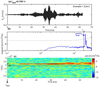 |
Fig. 1 Example of narrowband-type (category I, event no. 17) high-frequency wave. Electric field recorded by LPW instrument on MAVEN spacecraft is plotted as a function of time in milliseconds after the start time of this event, tstart = 06:45:29:160 hh:mm:ss:mss (in UT), fast Fourier spectra of these electric field variations and its spectrograms (frequency-time representation) are plotted in panels a, b, and c, respectively. The black dashed-dotted vertical line in panel b and horizontal line in panel c indicate the upper-hybrid wave estimated from ambient plasma parameters. The spectral peak is well above the 90% statistical significance marked by dashed grey line in panel b. Here, the length of electric field data is 62.5 ms. |
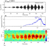 |
Fig. 2 Example of broadband-type (category II) high-frequency wave. Electric field recorded by LPW instrument on MAVEN spacecraft is plotted as a function of time in milliseconds after the start of this event (i.e., tstart), the fast Fourier spectra of these electric field variations and its spectrograms (frequency-time representation) are plotted in panels a, b, and c, respectively. This is example 2 (event no. 5) and its start time is 01:55:46:200 hh:mm:ss:mss (in UT). The black dashed-dotted vertical line in panel b and horizontal line in panel c indicate the upper-hybrid wave frequency estimated from ambient plasma parameters. The spectral peak is above the 90% statistical significance marked by dashed grey line in panel b. Here, the length of electric field data is 125 ms. |
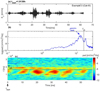 |
Fig. 3 Simultaneous narrowband-type and broadband-type (category III) high-frequency waves. Electric field recorded by LPW instrument on MAVEN spacecraft is plotted as a function of time in milliseconds after the start of this event (i.e., tstart), the fast Fourier spectra of these electric field variations and its spectrograms (frequency–time representation) are plotted in panels a, b, and c, respectively. This is example 3 (event no. 4) and its start time is 01:54:50:040 hh:mm:ss:mss (in UT). The black dashed-dotted vertical line in panel b and horizontal line in panel c indicate the upper-hybrid wave frequency estimated from ambient plasma parameters. The 90% statistical significance marked by dashed grey line in panel b. Here, the length of electric field data is 62.5 ms. |
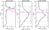 |
Fig. 4 Wave frequency as a function of average spectrogram power. (a) example 1 (category I), (b) example 2 (category II), and (c) example 3 (category III). The grey horizontal dashed lines indicate the lower and upper frequency limits for the observed wave. The magenta color dashed-dotted lines in each panel indicate the upper-hybrid (≈ electron plasma) frequency for each respective time of observation. For each wave mode, the frequency extent (or width), ∆f, is marked in each panel. |
4 Results
In the previous section, we detailed the features of 19 wave events observed in the Martian magnetosphere. These observations clearly indicate the presence of two types of waves namely narrowband-type (category I) and broadband-type (category II and III). The spectrogram shown in Figs. 2c and 3c features distinct patchy type structures with wider spread around the spectral peak frequency, whereas in Fig. 1c the wave power is continuous with a narrow frequency extent. Out of 19 wave events, 13 broadband-type events (category II and III) show such patchy appearance, whereas the remaining six narrowband-type (category I) are associated with continuous wave power.
In order to examine this repetitive behavior in broadband-type waves, we have plotted the average spectrogram power as a function of time in Fig. 5a for example 2. The time variation of 〈PSD〉 shows distinct peaks that represent periodic occurrence of patchy structures. The Fourier spectrum of this signal is shown in Fig. 5b, which reveals the presence of 11 ms periodicity in these structures. This exercise was repeated for all broadband-type wave events in order to estimate the repetitive periods. The distribution of estimated repetitive periods is shown in Fig. 5c. It is found that observed broadband-type waves possess repetitive periods in a close range of 8–14 ms (i.e., 75–125 Hz). This behavior is consistently seen in all broadband-type waves with an average repetitive period of 〈τ〉 = 10.6 ± 2 ms.
In order to identify and characterize the observed waves we examined the ambient plasma conditions and their occurrence region. We summarized the ambient plasma parameters for these 19 high-frequency wave events in Fig. 6. The altitude and local time of MAVEN spacecraft are plotted in Figs. 6a and e, respectively, where the occurrence of high-frequency wave events are marked in red color. It is evident that these waves are seen in the early morning hours at an altitude of ≈1400–3200 km. The remaining panels in Fig. 6 depict: (b) the ambient electron and ion densities; (c) the magnetic field; (d) the angle between the magnetic field and solar wind velocity vectors; (f) the solar wind plasma bulk speed; and (g) the electron and ion temperature as a function of altitude, for these 19 wave events. We found that the plasma density and velocity increase, whereas the magnetic field decreases with the altitude in the region where these high-frequency waves are observed. The angle between magnetic field and Ey is not estimated as we only have a single direction electric field. The ambient magnetic field and the solar wind velocity vectors are quasi-parallel with an average relative angle of θ = 46° ± 10°. Figure 6h shows the peak power spectral frequency as observed in the Fourier spectra of the electric field and the estimated upper-hybrid frequency (≈ electron plasma frequency) as a function of altitude. This indicates that the peak spectral frequency varies between 11 kHz and 24 kHz such that we have  for category II and III and, then,
  for category I.
The plasma parameters plotted in Fig. 6 are the calibrated key parameters derived from various instruments mounted on MAVEN and they are available at 4 s or 8 s resolution. The electron and ion densities shown in Fig. 6b are derived from SWEA and SWIA instruments on board MAVEN. The solar wind electron density (ne) represents the density of solar wind or magnetosheath electrons based on moments of the electron distribution after correcting for the spacecraft potential. Meanwhile, the total ion density (ni) is estimated from the on-board moment calculation of SWIA instrument by assuming 100% protons. We can see that there is a slight difference in ni and ne. We see that the measured ion density is lower when compared against the electron density. The assumption used in the estimate of ion density, that is, 100% population of H+ ions, may not be completely valid, which can result in an underestimation of ni as compared with ne. The passing of MAVEN spacecraft and the occurrence of these high-frequency waves are shown in Fig. 7a and b for two time intervals 1.5–2.1 UT and 6.2–6.9 UT. Mars does not have a global magnetic field of internal origin but it has some crustal magnetic field. Therefore, Mars and its upper atmosphere are directly exposed to the solar wind. This results in an induced magnetosphere through solar wind interactions with the upper atmosphere of Mars (Nagy et al. 2004; Ma et al. 2004). We used the model proposed by Trotignon et al. (2006) to obtain the location of Mars’ bow shock and magnetopause. These locations are depicted in Fig. 7. In this diagram, red color indicates the trajectory of MAVEN, while blue dots indicate the occurrence of high-frequency waves, which is localized in the dawn sector. MAVEN spacecraft crossed the magnetopause boundary, and then entered in the magnetosheath region, where the magnetic field is nearly steady. This is the region where the wave events are detected. We have checked the geographic longitude and latitude from the position of MAVEN. We noticed that these events were localized in the longitudinal and latitudinal zone of 216±30 and 31 ±10, respectively, where the crustal magnetic field is relatively weak compared to the southern hemisphere of Mars.
The characteristics of observed high-frequency wave events are summarized in Fig. 8. The peak spectral power as a function of peak spectral frequency is shown in Fig. 8a for narrowband-type waves, namely, category I (red), broadband-type wave, that is, category II and III (blue and black), and weak narrowband-type waves from category III (magenta). In the same way, the ratio of peak spectral frequency to upper-hybrid frequency (≈ electron plasma frequency) is plotted in Fig. 8b for these categories. It is clearly seen that the characteristics of narrowband-type and broadband-type wave events are distinct. The ratio  is greater than one for the narrowband-type wave events, whereas it is always less than one for the broadband-type waves. In general, the narrowband-type wave power is higher than that of the broadband-type wave but when the narrowband-type wave occurs simultaneously with the broadband-type wave its power diminishes. However, event no. 10 (category III) does not follow this trend (see Appendix A). For this event the narrowband-type wave occurs at the end of the broadband-type wave. This event appears as an outlier in the category III (narrowband-type) data points shown by magenta color in Fig. 8a.
Quantitatively, for narrowband-type events the frequency extent is given by 〈Δf〉 = 4.4 ± 1.4 kHz; low-end of the frequency spectrum, the peak frequency, and high-end of the spectrum are specified by 〈f1〉 = 19.8 ± 1.2 kHz,  , 〈fu〉 = 24.2 ± 2.2, respectively; peak power corresponds to 〈PSDpeak〉 = 7.2 × 10⁻⁶ (mVm−1)2 Hz−1; average lower-hybrid/plasma frequency is 〈fuh〉 ≈ 〈fpe〉 =18.6 kHz; and average cyclotron frequency is 〈fce〉 = 229 Hz. By the same token, quantitatively, for all broadband-band type events of category II and III, the corresponding quantities are specified by 〈Δf〉 = 10.3 ± 2.9 kHz, 〈f1〉 = 7.7 ± 2 kHz,
  , 〈fu〉 = 17.7 ± 1.9, 〈PSDpeak〉 = 6.9 × 10⁻⁷ (mVm−1)2 Hz−1, 〈fuh〉 ≈ 〈fpe〉 = 16.8 kHz, and 〈fce〉 = 269 Hz. All narrowband-type wave events seen simultaneously with broadband-type events of category III are characterized by the average peak power 〈PSDpeak〉 = 7.6 × 10⁻⁸. This indicates that the dominant mode in category III is the broadband-type wave. It is concluded that two different high-frequency wave modes have been observed in the magnetosphere region of Mars on 2015 February 9. In the next section (Sect. 5), we discuss the generation of possible wave modes by taking into account the ambient plasma conditions and information of observed waves.
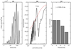 |
Fig. 5 Periodicities observed in broadband-type waves. Panel a shows average spectrogram power 〈PSD〉 as a function of time for event no. 5 shown in Fig. 2 (broadband-type wave, category II). Here, time is in milliseconds after the start time 01:55:46:200 hh:mm:ss:mss (in UT); panel b shows Fourier transform of average spectrogram power as a function of periods; and panel c shows the distribution of dominant repetitive periods observed in 13 broadband-type events of category II and III. The dominant repetitive period is estimated to be 10.6±2 ms. The red dashed line in panel b indicate the 90% statistical significance level for the Fourier spectra. |
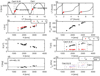 |
Fig. 6 Ambient plasma conditions in the wave occurrence region. Panel a shows MAVEN spacecraft altitude and panel e shows local time as a function of universal time (UT). The occurrences of high-frequency waves are marked with red “x” (b) Ion and electron density; (c) magnetic field strength; (d) angle between magnetic field and solar wind velocity vectors; (f) bulk solar wind speed; (g) ion and electron temperatures; (h) the peak frequency as seen in the spectra of observed electric field, |

 |
Fig. 7 MAVEN location and wave occurrence region. The trajectories of MAVEN spacecraft (red) in XY plane during time interval (a) 1.5–2.1 UT and (b) 6.25–6.85 UT around the Mars are shown. The modeled bow-shock and magnetopause boundary, obtained by using Trotignon et al. (2006), are shown. The occurrence of high-frequency fluctuations are marked with blue dots. |
5 Discussion
In the present paper, we discuss the observational characteristics of the narrowband-type and broadband-type high-frequency wave events in some detail. However, owing to the instrumental limitations, we are not able to confirm the direction of the electric field orientation with respect to the ambient magnetic field. These two types of wave events are observed to have the associated peak wave intensities situated above and below the upper-hybrid frequency (≈ electron plasma frequency) but it is difficult to identify the wave mode conclusively based on the frequency information alone. We have unidirectional electric field (Ey) measurements, which cannot be used to estimate the angle between the electric field and magnetic field vectors as other two components of the electric field might not be insignificant and such a condition cannot be confirmed without actual observations of Ex and Ez. The measurement of waves is also influenced by the antenna response. There could be some wavenumber-filtering due to antenna design and spacecraft orientation with respect to the local magnetic field. The high-resolution magnetic field observations are not available to verify electrostatic or electromagnetic nature of the observed wave phenomena. In such a scenario, the identification of wave mode is challenging.
From the information presented in the previous section, we can summarize the average values of ambient parameters as follows: 〈ni〉 ≈ 〈ne〉 = n = 3.75 ± 0.5/cc, Vsw = 166 ± 0.6 km s−1, 〈B〉 = 9.2–0.7 nT, 〈Te〉 = 16 ± 0.7 eV, 〈Ti〉 = 56 ± 9 eV, and 〈fpe〉 ≈ 〈fuh〉 = 17.3 ± 1 kHz. Here, we should note that electron thermal velocity is greater than ion thermal velocity. Such a plasma system supports the generation of high-frequency waves such as Langmuir and upper-hybrid waves. In the weakly magnetized plasma environment as in Martian magnetosphere,  . We noticed that all observed narrowband-type waves start from a frequency close to upper-hybrid (≈ electron plasma frequency) frequency. Therefore, we propose that narrowband-type events reported in this article could be possibly upper-hybrid waves or Langmuir waves. The upper-hybrid and Langmuir waves have maximum amplitude in a direction perpendicular and parallel to the ambient magnetic field, respectively.
As discussed earlier, narrowband-type waves start from a frequency slightly higher than the upper-hybrid (≈ electron plasma frequency). The gap between fuh and fl (start frequency of narrowband-type wave) is estimated to vary between 0 and 2.4 kHz. This tendency is consistent and seen for all narrowband events. Even the weak narrowband events seen in category III have a frequency marginally above fuh (≈ fpe). Such a frequency difference suggests the deviation of 0–1/cc in the electron density measurements. The consistent minor undercount of electron density could possibly be associated with both cold electron population with energy <3 eV, which is not measured by SWEA instrument.
In the Earth’s magnetosphere, the upper-hybrid waves are sometimes accompanied by several fluctuations in the multi-harmonic frequency bands of (n + 1/2) fce below and above the upper-hybrid frequency. However, in the case of Mars, such fluctuations in (n + 1/2)fce are not seen. This is because the characteristic frequency ratio in the case of Earth can be quite low, viz. fpe/fce on the order of 𝔖(10) or so, whereas in the Martian magnetosheath environment this ratio is much higher, fpe/fce ≈ 60–80, as noted above.
We also checked the possibility of frequency broadening due to Doppler shift. The ambient plasma parameters indicate that the solar wind speed is around 150 km s−1, the electron thermal speed is around 1620 km s−1. In general, the spacecraft speed is a few km s−1. As electron thermal velocity is much higher than the solar wind speed, the Doppler-shift effect can be ruled out. It is because high-frequency waves such as upper-hybrid and Lang-muir waves are characterized by phase speeds on the order of electron thermal velocity. It is possible to estimate that the phase speeds of these waves are much higher than the spacecraft speed or the solar wind speed. Consequently, the Doppler shift effect on the spectra is likely to be negligible for these high-frequency wave modes.
The property of the broadband-type waves warrants further mention. Explaining the broadband wave mode and 8–14 ms modulation associated with it is challenging. There is no obvious wave mode which can explain the broadband-type wave observations. It turns out that the ambient plasma parameters listed earlier is favorable to the existence of ion acoustic wave mode as Vthe ≫ Vthi. Ion-acoustic mode is a low frequency mode, which, if present, may be responsible for modulating the amplitude of high-frequency upper-hybrid or plasma frequency. Another possibility is the electron acoustic wave generation in the presence of some cold electron population. In earlier studies, it is shown that electron acoustic wave generation is supported in a three species plasma that comprise cold electron, hot electron and ions (Lakhina et al. 2008). A small population of cold electron (few eV) is sufficient to excite the electron acoustic wave mode. In such a plasma system, electron acoustic (fast) and ion acoustic wave mode (slow) are formed. Earlier simulation studies have shown that although the electron acoustic wave frequency extend up to and beyond the electron plasma frequency in a ω – k dispersion plot, the dominant wave power is situated much below the electron plasma frequency (Lotekar et al. 2019; Kakad & Kakad 2019). The wave power of electron acoustic mode decreases for larger wave number as we approach the electron plasma frequency, and the electron acoustic wave mode is found to be stronger around fpe/4. The phase speed of electron acoustic mode is around electron thermal speed, implying that the Doppler shift effects would be negligible. The observed broadband-type waves reported here start from around 8 kHz, which is around fpe/2, has a peak power around 14 kHz and it extend up to electron plasma frequency of 16.5 kHz and beyond. In such a situation, electron acoustic waves do not fully explain the broadband waves observations reported in this paper. The physical mechanism responsible for the generation of broadband-type waves and its 8–14 ms modulation is unexplained and requires further investigation.
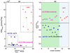 |
Fig. 8 Characteristics of observed high-frequency wave events. (a) Peak wave power of wave is plotted as a function of peak spectral frequency. (b) Ratio of peak spectral frequency to upper-hybrid frequency (≈ electron plasma frequency) for all 19 events categorized as narrowband-type (category I), broadband-type (category II and III), and weak narrowband-type seen simultaneously with broadband-type (category III) waves. |
6 Summary and conclusions
The high-frequency waves in the range of upper-hybrid frequency and/or plasma oscillation frequency are commonly reported in the Earth’s magnetosphere. The waves excited in the upper-hybrid frequency range are even suggested as being important for understanding the dynamic role of the electron diffusion region in magnetic reconnection (Jiang et al. 2019). Even in a quiet and quasi-uniform environment, upper-hybrid fluctuations may be involved in the steady-state wave-particle interaction with energetic electrons to sustain the quasi-turbulent equilibrium state (Yoon & Hwang 2020). Such high-frequency quasi-electrostatic fluctuations are observed by the RBSP (or Van Allen Probe) satellite in the Earth’s magnetosphere (Kurth et al. 2015; Yoon et al. 2018). In the case of Mars (and unlike Earth), the frequency ratio, fpe/fce is rather high, 60–70. In this paper, we have reported 19 high-frequency wave events that are observed in the Martian magnetosheath region on 2015 February 9. These high-frequency waves are observed in the early morning sector around 05 LT and seen for 30–300 ms in the spectrogram. All these high-frequency waves are observed in the magnetosheath region after the crossing of the magnetopause boundary by the MAVEN spacecraft. Based on their frequency extent they are mainly categorized as narrowbandtype (category I) and broadband-type waves (category II and III). Some broadband-type events are accompanied with extremely weak narrowband-type wave, which are counted under category III. These waves are observed in two separate altitudinal zones 1400–2200 km and 2600–3200 km at two time slots, 1.5–2.1 UT and 6.2–6.9 UT, respectively. In the first time slot, the broadband-type waves are dominant and they have frequency extent of Δf = 6–14 kHz with an average of 〈Δf〉 = 10.8 ± 2.8 kHz. It is noticed that the broadband-type waves start around 8 kHz, peak power is seen around 13.8 kHz, and then extend up to electron plasma frequency of 16.8 kHz or higher. These broadband-type waves have average peak spectral power density of 6.9 × 10⁻⁷ (mVm−1)2 Hz−1 around 13.8 kHz. The narrowband-type waves are observed in the second time slot and their frequency bandwidth is smaller, that is, 3.3 ± 1 kHz. These isolated narrowband-type waves have average peak spectral power density of 7.2 × 10⁻⁶ (mVm−1)2 Hz−1 around 21.8 kHz. The narrowband-type waves are always found to occur above the electron plasma frequency, which is estimated to be around 18.6 kHz at those altitudes.
As the magnetic field is weak, the upper-hybrid and Lang-muir wave frequencies are in close proximity (i.e., fuh ≈ fpe). We can see that the narrowband-type and broadband-type waves have peak spectral frequency above and below electron plasma frequency (or upper-hybrid frequency), respectively. The narrowband-type wave are speculated to be upper-hybrid or Langmuir type wave modes. Unlike continuous narrowband-type waves, the broadband-type waves possess distinct (repetitive) patchy structures in the dynamic spectrum, with the spectral power concentrated below the upper-hybrid or Langmuir frequency. This distinct observational feature is seen in all broadband-type wave events and their modulation periods vary in a close range of 8–14 ms (i.e., 70–125 Hz). There is no obvious wave mode which can explain the broadband-type. Information regarding the wave direction is limited due to availability of only one directional electric field. In such a scenario, the physical mechanism responsible for the generation of the broadband-type wave mode and its modulation remain largely unexplained and requires further theoretical investigations. The present study provides conclusive evidence for the occurrence of high-frequency waves in the Martian magnetosheath. Waves such as the ones observed and reported in this paper could play a significant role in wave-particle interaction processes in the Martian plasma environment, but it is of equal importance that the detection and detailed analysis of the high-frequency plasma waves and fluctuations in the Martian environment, as reported in the present paper, are unprecedented, as such, the present study has an clear intrinsic scientific value.
Acknowledgements
The data used in the present study are available on the Planetary Data System (https://pds-ppi.igpp.ucla.edu/). The authors are thankful to L. Andersson, for LPW/MAVEN data. The authors thank J.E.P. Connerney for providing access to MAG/MAVEN data, D.L. Mitchell for SWEA/MAVEN data, J.S. Halekas for SWIA/MAVEN data and P.A. Dunn for key parameters. A.K. and B.K. acknowledge support from IIG, India for research funding under IIG/EPTOS/2021-2024. I.K. acknowledges financial support from Khalifa University’s Space and Planetary Science Center under grant no. KU-SPSC-8474000336, as well as from project FSU-2021-012/8474000352, funded by Khalifa University of Science and Technology, Abu Dhabi, UAE. P.H.Y. acknowledges NSF Grant 2203321, NASA Grant 80NSSC23K0662, and DOE (FES) Award DE-SC0022963 through the NSF/DOE Partnership in Basic Plasma Science and Engineering to the University of Maryland. This study was finalized during visit of A.K. to RISH, Kyoto University, Japan. A.K. gratefully acknowledges RISH Kyoto University Japan for the hospitality provided during his visit.
Appendix A Wave observations
We have observed a total of 19 high-frequency events in the Martian magnetosphere. All these events are numbered from 1-19 based on their occurrence in time domain. One event from each category is shown in the article as an example. The remaining 13 wave events are shown in this section. In each of the following figures, the upper panel shows the Ey component of the electric field in spacecraft coordinate system. The middle and lower panels, respectively, show the Fourier transform and spectrogram of the measured electric field. The start time (in UT) for each event is mentioned in respective figure.
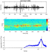 |
Fig. A.1 Event no. 1; category III |
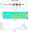 |
Fig. A.2 Event no. 2; category III |
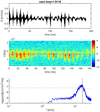 |
Fig. A.3 Event no. 3; category III |
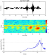 |
Fig. A.4 Event no. 6; category III |
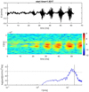 |
Fig. A.5 Event no. 7; category III |
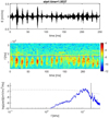 |
Fig. A.6 Event no. 8; category III |
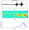 |
Fig. A.7 Event no. 9; category II |
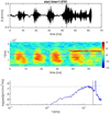 |
Fig. A.8 Event no. 10; category III |
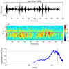 |
Fig. A.9 Event no. 11; category III |
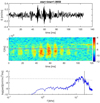 |
Fig. A.10 Event no. 12; category II |
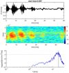 |
Fig. A.11 Event no. 13; category II |
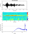 |
Fig. A.12 Event no. 14; category I |
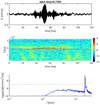 |
Fig. A.13 Event no. 15; category I |
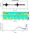 |
Fig. A.14 Event no. 16; category I |
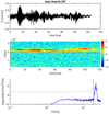 |
Fig. A.15 Event no. 18; category I |
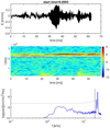 |
Fig. A.16 Event no. 19; category I |
References
- Andersson, L., Ergun, R., Delory, G., et al. 2015, Space Sci. Rev., 195, 173 [NASA ADS] [CrossRef] [Google Scholar]
- Bale, S., Kellogg, P., Larsen, D., et al. 1998, Geophys. Res. Lett., 25, 2929 [NASA ADS] [CrossRef] [Google Scholar]
- Connerney, J., Espley, J., Lawton, P., et al. 2015, Space Sci. Rev., 195, 257 [NASA ADS] [CrossRef] [Google Scholar]
- Filbert, P. C., & Kellogg, P. J. 1979, J. Geophys. Res., 84, 1369 [NASA ADS] [CrossRef] [Google Scholar]
- Gilman, D. L., Fuglister, F. J., & Mitchell, J. 1963, J. Atmos. Sci., 20, 182 [NASA ADS] [CrossRef] [Google Scholar]
- Graham, D. B., Vaivads, A., Khotyaintsev, Y. V., et al. 2018, J. Geophys. Res. Space Phys., 123, 2630 [NASA ADS] [CrossRef] [Google Scholar]
- Graham, D., Khotyaintsev, Y. V., André, M., et al. 2022, Nat. Commun., 13, 1 [Google Scholar]
- Grard, R., Pedersen, A., Klimov, S., et al. 1989, Nature, 341, 607 [NASA ADS] [CrossRef] [Google Scholar]
- Gunell, H., Maggiolo, R., Nilsson, H., et al. 2018, A & A, 614, A3 [Google Scholar]
- Guo, Z., Liu, Y., Fu, H., et al. 2022, ApJ, 933, 128 [NASA ADS] [CrossRef] [Google Scholar]
- Halekas, J., Taylor, E., Dalton, G., et al. 2015, Space Sci. Rev., 195, 125 [CrossRef] [Google Scholar]
- Harada, Y., Andersson, L., Fowler, C., et al. 2016, J. Geophys. Res. Space Phys., 121, 9717 [NASA ADS] [CrossRef] [Google Scholar]
- Issautier, K., Moncuquet, M., Meyer-Vernet, N., Hoang, S., & Manning, R. 2001, Astron. Space Sci., 277, 309 [NASA ADS] [CrossRef] [Google Scholar]
- Jiang, K., Huang, S., Yuan, Z., et al. 2019, ApJ, 881, L28 [NASA ADS] [CrossRef] [Google Scholar]
- Kakad, A., & Kakad, B. 2019, Phys. Plasmas, 26 [Google Scholar]
- Kakad, A., Kakad, B., Omura, Y., et al. 2019, J. Geophys. Res. Space Phys., 124, 1992 [NASA ADS] [CrossRef] [Google Scholar]
- Kakad, B., Kakad, A., Aravindakshan, H., & Kourakis, I. 2022, ApJ, 934, 126 [NASA ADS] [CrossRef] [Google Scholar]
- Kretzschmar, M., Chust, T., Krasnoselskikh, V., et al. 2021, A & A, 656, A24 [NASA ADS] [CrossRef] [EDP Sciences] [Google Scholar]
- Kurth, W., De Pascuale, S., Faden, J., et al. 2015, J. Geophys. Res. Space Phys., 120, 904 [CrossRef] [Google Scholar]
- Lakhina, G. S., Kakad, A. P., Singh, S. V., & Verheest, F. 2008, Phys. Plasmas, 15, 062903-062903-7 [NASA ADS] [CrossRef] [Google Scholar]
- Li, W.-Y., Khotyaintsev, Y. V., Tang, B.-B., et al. 2021, Geophys. Res. Lett., 48, e2021GL093164 [CrossRef] [Google Scholar]
- Lotekar, A., Kakad, A., & Kakad, B. 2019, J. Geophys. Res. Space Phys., 124, 6896 [NASA ADS] [CrossRef] [Google Scholar]
- Lundin, R., Winningham, D., Barabash, S., et al. 2006, Science, 311, 980 [NASA ADS] [CrossRef] [Google Scholar]
- Ma, Y., Nagy, A. F., Sokolov, I. V., & Hansen, K. C. 2004, J. Geophys. Res. Space Phys., 109 [Google Scholar]
- Malaspina, D. M., Goodrich, K., Livi, R., et al. 2020, Geophys. Res. Lett., 47, e2020GL090115 [CrossRef] [Google Scholar]
- Meyer-Vernet, N. 1979, J. Geophys. Res., 84, 5373 [Google Scholar]
- Meyer-Vernet, N., & Perche, C. 1989, J. Geophys. Res., 94, 2405 [NASA ADS] [CrossRef] [Google Scholar]
- Mitchell, D., Mazelle, C., Sauvaud, J.-A., et al. 2016, Space Sci. Rev., 200, 495 [NASA ADS] [CrossRef] [Google Scholar]
- Moncuquet, M., Lecacheux, A., Meyer-Vernet, N., Cecconi, B., & Kurth, W. S. 2005, Geophys. Res. Lett., 32, L20S02 [Google Scholar]
- Mozer, F., Bonnell, J., Hanson, E., Gasque, L., & Vasko, I. 2021a, ApJ, 911, 89 [CrossRef] [Google Scholar]
- Mozer, F. S., Vasko, I. Y., & Verniero, J. 2021b, ApJ, 919, L2 [NASA ADS] [CrossRef] [Google Scholar]
- Nagy, A., Winterhalter, D., Sauer, K., et al. 2004, Space Sci. Rev., 111, 33 [NASA ADS] [CrossRef] [Google Scholar]
- Pérez-de Tejada, H. 1987, J. Geophys. Res. Space Phys., 92, 4713 [CrossRef] [Google Scholar]
- Pickett, J. 2021, J. Geophys. Res. Space Phys., 126, e2021JA029548 [NASA ADS] [CrossRef] [Google Scholar]
- Romanelli, N., Modolo, R., Leblanc, F., et al. 2018, Geophys. Res. Lett., 45, 7891 [NASA ADS] [CrossRef] [Google Scholar]
- Saur, J., Janser, S., Schreiner, A., et al. 2018, J. Geophys. Res. Space Phys., 123, 9560 [NASA ADS] [CrossRef] [Google Scholar]
- Strangeway, R. 1991, Space Sci. Rev., 55, 275 [CrossRef] [Google Scholar]
- Tao, J., Ergun, R., Newman, D., et al. 2012, J. Geophys. Res. Space Phys., 117, A03106 [NASA ADS] [Google Scholar]
- Thaller, S. A., Andersson, L., Schwartz, S. J., et al. 2022, J. Geophys. Res. Space Phys., e2022JA030374 [CrossRef] [Google Scholar]
- Trotignon, J. G., Grard, R., & Savin, S. 1991, J. Geophys. Res. Space Phys., 96, 11253 [NASA ADS] [CrossRef] [Google Scholar]
- Trotignon, J., Mazelle, C., Bertucci, C., & Acuña, M. 2006, Planet. Space Sci., 54, 357 [NASA ADS] [CrossRef] [Google Scholar]
- Vaisberg, O., Ermakov, V., Shuvalov, S., et al. 2017, Planet. Space Sci., 147, 28 [NASA ADS] [CrossRef] [Google Scholar]
- Vaisberg, O., Ermakov, V., Shuvalov, S., et al. 2018, J. Geophys. Res. Space Phys., 123, 2679 [NASA ADS] [CrossRef] [Google Scholar]
- Wang, J., Yu, J., Xu, X., et al. 2021, Geophys. Res. Lett., 48, e2021GL095426 [CrossRef] [Google Scholar]
- Yoon, P. H., & Hwang, J. 2020, J. Geophys. Res., 125, e2019JA027748 [CrossRef] [Google Scholar]
- Yoon, P. H., Hwang, J., Lopez, R. A., Kim, S., & Lee, J. 2018, J. Geophys. Res. Space Phys., 123, 5356 [NASA ADS] [CrossRef] [Google Scholar]
- Zhao, L.-L., Zank, G., He, J., et al. 2021, ApJ, 922, 188 [NASA ADS] [CrossRef] [Google Scholar]
All Figures
|
Fig. 1 Example of narrowband-type (category I, event no. 17) high-frequency wave. Electric field recorded by LPW instrument on MAVEN spacecraft is plotted as a function of time in milliseconds after the start time of this event, tstart = 06:45:29:160 hh:mm:ss:mss (in UT), fast Fourier spectra of these electric field variations and its spectrograms (frequency-time representation) are plotted in panels a, b, and c, respectively. The black dashed-dotted vertical line in panel b and horizontal line in panel c indicate the upper-hybrid wave estimated from ambient plasma parameters. The spectral peak is well above the 90% statistical significance marked by dashed grey line in panel b. Here, the length of electric field data is 62.5 ms. |
| In the text | |
|
Fig. 2 Example of broadband-type (category II) high-frequency wave. Electric field recorded by LPW instrument on MAVEN spacecraft is plotted as a function of time in milliseconds after the start of this event (i.e., tstart), the fast Fourier spectra of these electric field variations and its spectrograms (frequency-time representation) are plotted in panels a, b, and c, respectively. This is example 2 (event no. 5) and its start time is 01:55:46:200 hh:mm:ss:mss (in UT). The black dashed-dotted vertical line in panel b and horizontal line in panel c indicate the upper-hybrid wave frequency estimated from ambient plasma parameters. The spectral peak is above the 90% statistical significance marked by dashed grey line in panel b. Here, the length of electric field data is 125 ms. |
| In the text | |
|
Fig. 3 Simultaneous narrowband-type and broadband-type (category III) high-frequency waves. Electric field recorded by LPW instrument on MAVEN spacecraft is plotted as a function of time in milliseconds after the start of this event (i.e., tstart), the fast Fourier spectra of these electric field variations and its spectrograms (frequency–time representation) are plotted in panels a, b, and c, respectively. This is example 3 (event no. 4) and its start time is 01:54:50:040 hh:mm:ss:mss (in UT). The black dashed-dotted vertical line in panel b and horizontal line in panel c indicate the upper-hybrid wave frequency estimated from ambient plasma parameters. The 90% statistical significance marked by dashed grey line in panel b. Here, the length of electric field data is 62.5 ms. |
| In the text | |
|
Fig. 4 Wave frequency as a function of average spectrogram power. (a) example 1 (category I), (b) example 2 (category II), and (c) example 3 (category III). The grey horizontal dashed lines indicate the lower and upper frequency limits for the observed wave. The magenta color dashed-dotted lines in each panel indicate the upper-hybrid (≈ electron plasma) frequency for each respective time of observation. For each wave mode, the frequency extent (or width), ∆f, is marked in each panel. |
| In the text | |
|
Fig. 5 Periodicities observed in broadband-type waves. Panel a shows average spectrogram power 〈PSD〉 as a function of time for event no. 5 shown in Fig. 2 (broadband-type wave, category II). Here, time is in milliseconds after the start time 01:55:46:200 hh:mm:ss:mss (in UT); panel b shows Fourier transform of average spectrogram power as a function of periods; and panel c shows the distribution of dominant repetitive periods observed in 13 broadband-type events of category II and III. The dominant repetitive period is estimated to be 10.6±2 ms. The red dashed line in panel b indicate the 90% statistical significance level for the Fourier spectra. |
| In the text | |
|
Fig. 6 Ambient plasma conditions in the wave occurrence region. Panel a shows MAVEN spacecraft altitude and panel e shows local time as a function of universal time (UT). The occurrences of high-frequency waves are marked with red “x” (b) Ion and electron density; (c) magnetic field strength; (d) angle between magnetic field and solar wind velocity vectors; (f) bulk solar wind speed; (g) ion and electron temperatures; (h) the peak frequency as seen in the spectra of observed electric field, |
| In the text | |
|
Fig. 7 MAVEN location and wave occurrence region. The trajectories of MAVEN spacecraft (red) in XY plane during time interval (a) 1.5–2.1 UT and (b) 6.25–6.85 UT around the Mars are shown. The modeled bow-shock and magnetopause boundary, obtained by using Trotignon et al. (2006), are shown. The occurrence of high-frequency fluctuations are marked with blue dots. |
| In the text | |
|
Fig. 8 Characteristics of observed high-frequency wave events. (a) Peak wave power of wave is plotted as a function of peak spectral frequency. (b) Ratio of peak spectral frequency to upper-hybrid frequency (≈ electron plasma frequency) for all 19 events categorized as narrowband-type (category I), broadband-type (category II and III), and weak narrowband-type seen simultaneously with broadband-type (category III) waves. |
| In the text | |
|
Fig. A.1 Event no. 1; category III |
| In the text | |
|
Fig. A.2 Event no. 2; category III |
| In the text | |
|
Fig. A.3 Event no. 3; category III |
| In the text | |
|
Fig. A.4 Event no. 6; category III |
| In the text | |
|
Fig. A.5 Event no. 7; category III |
| In the text | |
|
Fig. A.6 Event no. 8; category III |
| In the text | |
|
Fig. A.7 Event no. 9; category II |
| In the text | |
|
Fig. A.8 Event no. 10; category III |
| In the text | |
|
Fig. A.9 Event no. 11; category III |
| In the text | |
|
Fig. A.10 Event no. 12; category II |
| In the text | |
|
Fig. A.11 Event no. 13; category II |
| In the text | |
|
Fig. A.12 Event no. 14; category I |
| In the text | |
|
Fig. A.13 Event no. 15; category I |
| In the text | |
|
Fig. A.14 Event no. 16; category I |
| In the text | |
|
Fig. A.15 Event no. 18; category I |
| In the text | |
|
Fig. A.16 Event no. 19; category I |
| In the text | |
Current usage metrics show cumulative count of Article Views (full-text article views including HTML views, PDF and ePub downloads, according to the available data) and Abstracts Views on Vision4Press platform.
Data correspond to usage on the plateform after 2015. The current usage metrics is available 48-96 hours after online publication and is updated daily on week days.
Initial download of the metrics may take a while.