| Issue |
A&A
Volume 696, April 2025
|
|
|---|---|---|
| Article Number | A39 | |
| Number of page(s) | 21 | |
| Section | Astronomical instrumentation | |
| DOI | https://doi.org/10.1051/0004-6361/202450312 | |
| Published online | 01 April 2025 | |
Mutual impedance experiments in a magnetized plasma
A numerical investigation of magnetic field and temperature anisotropy effects on a space plasma diagnostic
1
Laboratoire de Physique et Chimie de l’Environnement et de l’Espace (LPC2E), CNRS, Université d’Orléans,
Orléans,
France
2
LESIA, Observatoire de Paris, PSL Research University, CNRS, Sorbonne Université, UPMC, Université Paris Diderot, Sorbonne Paris Cité,
Meudon,
France
3
Laboratoire Lagrange, OCA, UCA, CNRS,
Nice,
France
4
LPP, Sorbonne Université, CNRS, Ecole Polytechnique,
91128
Palaiseau,
France
5
Dipartimento di Fisica, Università di Pisa,
Pisa,
Italy
6
Laboratoire Plasma et Conversion d’Energie (LAPLACE), CNRS, Université de Toulouse,
Toulouse,
France
★ Corresponding author; This email address is being protected from spambots. You need JavaScript enabled to view it.
Received:
10
April
2024
Accepted:
12
August
2024
Abstract
Context. A mutual impedance experiment is an active in situ space plasma diagnostic that is used to determine the electron density and temperature. Such parameters are inferred from the mutual impedance spectrum measured between a pair of electric antennas embedded in the plasma. This state-of-the-art plasma diagnostic technique is limited to unmagnetized plasmas; that is, ones with a plasma frequency much larger than the electron cyclotron frequency. This limit is not expected to be valid in the plasma environment surrounding magnetized planets such as Mercury and Jupiter that will be explored by the ESA JUICE and joint ESA/JAXA Bepi-Colombo missions.
Aims. The goal of this work is to extend the mutual impedance diagnostic technique to magnetized plasmas, focusing on measurements of the electron density and temperature, and to extend it to the electron temperature anisotropy.
Methods. To achieve this, we developed the first quantitative three-dimensional instrumental model for mutual impedance experiments in a magnetized plasma. This model is valid for arbitrary values of the electron temperature and magnetic field. Our model is based on the linearized Vlasov-Maxwell coupled system of equations. We numerically computed the electric potential generated and simultaneously measured by the mutual impedance experiment, in order to compute the mutual impedance spectrum in a magnetized plasma.
Results. First, we identify in the numerical mutual impedance spectra a number of local spectral signatures, associated with characteristic frequencies that can be used for plasma diagnostics. We show how the magnetic field strength and direction modify such spectral signatures. Second, we show that electron-neutral collision smooth out the spectrum, as long as the scattering-to-plasma frequency ratio is greater than 10−3 . Below such a value, mutual impedance experiments are insensitive to electron-neutral scattering and the plasma can be considered collisionless. Third, we show that the electron temperature directly controls the amplitude of the mutual impedance spectra, so that such behavior can be used as an electron temperature diagnostic. Fourth, we explore for the first time the possibility of diagnosing electron temperature anisotropies with mutual impedance experiments. We show how an electron temperature anisotropy significantly modifies the mutual impedance spectral signatures, as a result of the modified propagation of the electron Bernstein waves generated by the experiment.
Conclusions. The results of our model, in terms of plasma diagnostics, are discussed in terms of the propagation properties in a magnetized plasma of the electrostatic waves generated by the active mutual impedance experiment. The results of our model will significantly extend the plasma diagnostic capabilities of the current and future mutual impedance experiment such as the PWI/AM2P experiment on board BepiColombo and the RPWI/MIME experiment on board JUICE.
Key words: magnetic fields / plasmas / waves / instrumentation: miscellaneous / methods: numerical / planets and satellites: magnetic fields
© The Authors 2025
 Open Access article, published by EDP Sciences, under the terms of the Creative Commons Attribution License (https://creativecommons.org/licenses/by/4.0), which permits unrestricted use, distribution, and reproduction in any medium, provided the original work is properly cited.
This article is published in open access under the Subscribe to Open model. This email address is being protected from spambots. You need JavaScript enabled to view it. to support open access publication.
1 Introduction
Mutual impedance experiments are a type of in situ space plasma diagnostic used to infer the electron density and temperature, and they measure the mutual impedance spectrum between two electric antennas embedded in the plasma. This measurement is performed by generating an electric perturbation within the plasma using one or several antennas, while another (pair of) antennas simultaneously measures the electric field. By changing the frequency of the perturbation, the characteristic resonant frequencies of the plasma are identified, which in turn depend on various plasma parameters. One example of the resonances explored by a mutual impedance experiment is the plasma frequency. In the limit of a homogeneous, isotropic, unmagnetized plasma, with a Maxwellian electron distribution, a single resonance is present in the mutual impedance spectrum at the plasma frequency of  , where qe and me are the charge and mass of the electron, respectively, and ɛ0 is the vacuum permittivity. Such a resonance provides a measurement of the electron density, ne.
Various past space missions have embarked on mutual impedance experiments to study the Earth’s ionosphere (e.g. FR-1; Storey et al. 1969, DRAGON-3; Beghin 1971, CISASPE; Chasseriaux et al. 1972, PORCUPINE; Haeusler et al. 1982) and magnetosphere (e.g. GEOS-1; Décréau et al. 1978, ARCAD-3; Béghin et al. 1982, Viking; Perraut et al. 1990; Bahnsen et al. 1988), as well as the atmosphere of Titan (Huygens probe Hamelin et al. 2007) and the plasma environment of the comet 67P-CG (Rosetta RPC-MIP; Trotignon et al. 2007). Mutual impedance experiments are also part of the scientific payload of current and future space missions; notably, PWI/AM2P (Kasaba et al. 2020) on board the ESA/JAXA BepiColombo mission (Benkhoff et al. 2021), RPWI/MIME (Fischer et al. 2021) on board the ESA JUICE mission (Grasset et al. 2013), and DFP/COMPLIMENT (De Keyser et al. 2021) on board the ESA Comet Interceptor mission (Snodgrass & Jones 2019). On top of these large-scale missions, instrumental effort is being dedicated to adapting mutual impedance instruments for nanosatellite platforms (Bucciantini et al. 2023a). An instrumental model is needed in order to be able to use mutual impedance experiments as a plasma diagnostic. This is because an instrumental model provides the connection between the mutual impedance spectrum and the plasma parameters. If the magnetic field is negligible, and considering a Maxwellian distribution for the electrons, the mutual impedance spectrum, Z(f), depends on the plasma electron density and temperature; namely, Z (f) = Z (f, ne, Te).
The BepiColombo and JUICE missions will explore the magnetospheric plasma environments of Mercury and the Jupiter system; notably, its moons Europa, Callisto, and Ganymede. The non-negligible planetary magnetic field has a significant impact on the mutual impedance experiments, and therefore on the plasma diagnostics (Décréau et al. 1987). Considering an anisotropic Maxwellian distribution for the electrons, the mutual impedance spectrum is expressed as Z (f) = Z (f, ne, Te⊥, Te‖,B). In other words, the space of the parameters influencing mutual impedance experiments is increased by the presence of a magnetic field.
Current state-of-the-art mutual impedance modeling mostly addresses the limit of an unmagnetized plasma, and was most recently conducted in the context of the Rosetta mission. Gilet et al. (2017) modeled the effects of a Maxwellian and the sum of two Maxwellians’ electron distribution function on the RPC-MIP mutual impedance experiment. The sum of two Maxwellians’ electron distribution results in the presence of two resonances in the mutual impedance spectrum. The Gilet et al. (2017) model was extended in Wattieaux et al. (2019, 2020) to take into account both (i) the effects of the boundary conditions given by the conductive spacecraft, and (ii) the plasma inhomogeneity created around the spacecraft by charging effects (Grard et al. 1983). The effect of a Kappa electron distribution function was explored in Gilet et al. (2019) in the context of the BepiColombo mission. All the models previously described for an unmagnetized plasma are based on the linear approximation, which means considering the first-order perturbation of the electric field and distribution function of the plasma. Vlasov-Poisson simulations have been used in Bucciantini et al. (2022) and Bucciantini et al. (2023b) to characterize the influence of nonlinear effects on mutual impedance experiments and to give an upper limit on the emission intensity of mutual impedance experiments, as well as to explore the effects on mutual impedance measurements of plasma inhomogeneity around the spacecraft.
It has been estimated experimentally in Decreau-Prior (1983) that the magnetic field significantly perturbs mutual impedance experiments if fpe / fce < 3, where  is the electron cyclotron frequency and B is the strength of the magnetic field. In the magnetized case − Z (f) = Z (f, ne, Te,⊥, Te,‖, B) – multiple local maxima each associated with the different plasma eigenmodes are present in the mutual impedance spectrum. The way these eigenmodes are observed in the mutual impedance spectrum depends upon the plasma parameters, including the plasma density, the electron temperature, the strength of the magnetic field, and its direction relative to the antennas. This fact is expressed in the dependency of the mutual impedance spectrum upon the plasma parameters, Z (f) = Z (f, ne, Te,⊥, Te,‖, B). In the following, we list the characteristic frequencies relevant for mutual impedance experiments, while a more in-detail description of the plasma eigenmodes is given in Sect. 3. We consider here only the electrostatic modes that are those of interest for mutual impedance experiments, as is discussed and justified in Sect. 3. In the following list of characteristic frequencies, we work under the isotropic hypotheses; that is, a Maxwellian electron distribution. The same modes are also present in the anisotropic case, with a different electron perpendicular and parallel temperature.
First, in the limit case of parallel propagation, k × B = 0, the plasma resonances tend to the ones present in an unmagnetized plasma. The least damped resonance (Derfler & Simonen 1969) is the Langmuir wave, and is located around the plasma frequency in the mutual impedance spectrum. Previous works (Pottelette et al. 1981; Decreau-Prior 1983) showed that in the case of weak magnetization, fce /fpe ≃ 1, a maximum in the mutual impedance spectrum is not evident at this frequency. Second, in the limit case of perpendicular propagation, k ⋅ B = 0, the plasma resonances are the electron Bernstein waves (Bernstein 1958). These resonances are present only at specific frequency bands, meeting the condition nfce ≤ f ≤ fqn for n ϵ ℕ, where fqn is the frequency for which the mode group velocity is zero, ∂kf(fqn) = 0. In the mutual impedance spectrum, the fqn frequencies correspond to a series of local maxima that increase in amplitude if the emitting-receiving direction gets close to perpendicular to the magnetic field. This is because Bernstein modes are heavily damped when not propagating perpendicular to the magnetic field. Third, in the general case of oblique propagation, the main resonance of interest to mutual impedance experiments is given by the upper-hybrid surface (Andre 1985), which gives a frequency around the upper-hybrid frequency,  (Décréau et al. 1987).
Previous works modeled the mutual impedance spectrum, Z(f), in the case of a non-negligible magnetic field (i.e., fce/fpe > 0.3), concentrating on specific physical limits of validity. Storey et al. (1969) computed the analytical expression of the mutual impedance spectrum under the assumption of a fluid cold plasma for a pair of dipolar spherical antennas. This was later used in Fisher & Gould (1971) to analyze laboratory experiments. Fluid cold plasma approximation does not consider the effects of the electron temperature, and therefore of Landau damping of the signal propagating in the plasma. In the context of mutual impedance experiments, this approximation is valid only in the limit of λDe ≪ l, where λDe is the Debye length and l is the distance between the emitting and receiving antennas. Kuehl (1973) numerically computed the electric potential generated by a mutual impedance experiment under the assumption of a kinetic plasma, with a small nonzero temperature. This was done by taking the limit of the small electron gyro-radius, rLe ≪ l, and the small Debye length, λDe ≪ l. Such results were used by Rohde et al. (1993) to analyze the results of ionospheric mutual impedance experiments. Pottelette et al. (1981) performed a numerical calculation of the mutual impedance spectrum under the assumption of a kinetic plasma with a Maxwellian electron distribution and a quadrupolar antenna perpendicular to the ambient magnetic field. The results of Pottelette et al. (1981) were used to interpret the measurements from the PORCUPINE ionospheric rocket campaign (Storey et al. 1981) and the GEOS-1 satellite (Décréau et al. 1978). The assumptions of these past models constrain their current and future mutual impedance experiments; in particular, the magnetized environment of Earth, Mercury, and the Jupiter system, explored among others by BepiColombo and JUICE. For this reason, the model we present in this work relaxes these assumptions, as we take into account the effects of a variable Debye length, from small up to the same size as the mutual impedance antennas, as well as an arbitrary orientation and strength of the magnetic field.
The main goal of this work is to provide a diagnostic for the plasma density and electron temperature(s) from mutual impedance experiments in a magnetized plasma, as well as for the electron temperature anisotropy. Additionally, an estimation of the magnetic field direction and amplitude is derived. This was achieved by developing the first generic instrumental model of mutual impedance experiments in a magnetized plasma, based on linearized Vlasov-Maxwell equations. The expression of the electric potential in the plasma was solved numerically in order to retrieve the plasma response as a function of plasma density, temperature(s), magnetic field amplitude, and direction relative to the antenna. This electric potential was used to construct the compute mutual impedance spectrum, Z (f, ne, Te,⊥, Te,‖, B).
The paper is organized as follows. The model of magnetized mutual impedance experiments is defined in Sect. 2. A detailed description of the plasma modes is given in Sect. 3. The implementation of the electric potential numerical calculation is described in Appendix A and validated in Appendix B. The results of the numerical calculation are presented in Sect. 4 for a monopolar (Sect. 4.1) and dipolar (Sect. 4.2) antenna. We also consider the effects of an electron temperature anisotropy in Sect. 5, and of electron-neutral scattering in Sect. 6. We summarize our conclusions in Sect. 7.
2 Definition of the analytical model for mutual impedance experiments in a magnetized plasma
A schematic version of a mutual impedance experiment is presented in Fig. 1, in which the two electrodes of the emitting (resp. receiving) antenna are indicated as Eı and E2 (resp. R1 and R2). The measurement of mutual impedance between the two antennas was performed by imposing an alternating electric current, I (t), of fixed angular frequency, ω, and constant amplitude, I, between the two electrodes, E1 and E2. Simultaneously, the electric potential difference, V (t), between the two receiving electrodes, Rı and R2 , was measured. The mutual impedance is defined as the ratio of the Fourier transforms of the electric potential, ℱ[V](ω), to the Fourier transform of the current, ℱ[I](ω), at the emitted angular frequency, ω. The mutual impedance spectrum was measured by performing a succession of mutual impedance measurements, varying the angular frequency, ω (Storey et al. 1969). This type of emitted signal is referred to as a “frequency sweep.” Other types of emission are explored in Bucciantini et al. (2023a), but their modeling in the case of a magnetized plasma is out of the scope of this work. The result of a mutual impedance experiment is in the form Z(ω) = ℱ[V](ω)/ℱ[I](ω), and is typically normalized to its value in vacuum, Z0(ω). This is done in order to isolate the variations of the mutual impedance spectrum due to the presence of the plasma. The normalized mutual impedance reads:
 (1)
(1)
where V0 is the electric potential measured in vacuum. The modeling of mutual impedance experiments therefore requires the computation of Z/Z0 as a function of the angular frequency, ω, as is presented in Eq. (1). In the following, we define the model used in this work to describe a mutual impedance experiment. From this model, an integral expression for Eq. (1) is obtained, as a function of the plasma parameters.
The model is based on a number of hypotheses, listed below. First, the charging time of the electrodes (Eı , E2 , Rı , R2) is supposed to be negligible compared to the oscillation period of the emitted signal, 2π/ω. Second, the plasma response is supposed to be linear. This is justified by the fact that the energy of the electric field generated inside the plasma is much smaller than the electron thermal energy (Bucciantini et al. 2022). Third, the plasma ions are considered as a fixed, neutralizing charge background. This is because the frequencies relevant to mutual impedance experiments are around the plasma frequency, and are therefore much higher than the ion characteristic frequencies, such as the ion plasma frequency,  , and the ion cyclotron frequency,
  , where qi and mi are the change and mass of the ion, respectively. Fourth, the plasma is considered as collisionless at the temporal and spatial scale of a mutual impedance experiment. This justifies the use of the Vlasov equation to model the electrons in the plasma. Nonetheless, electron-neutral collisions are added in our model for numerical regularization purposes (as is discussed in Sect. 6). Fifth, the background magnetic field is considered as homogeneous at the spatial scale of the mutual impedance experiment. In the rest of this work, a cylindrical coordinate system is chosen as to have the z-axis parallel to the background magnetic field, B = Bz. Sixth, the total magnetic field present inside the plasma is supposed to be constant, meaning that ∂tB = 0. This hypothesis is referred to as the electrostatic approximation. It is justified by the fact that, in the range of parameters of interest for mutual impedance experiments, electromagnetic waves have wavelengths much larger than the ones of electrostatic waves. A discussion of the validity of this assumption is presented in the next section, Sect. 3.
Under these hypotheses, the time-and-space Fourier- transformed electric potential reads:
 (2)
(2)
where ρext.(ω, k) is the electric charge distribution that models the electrodes, Eı and E2, ɛL(ω, k) is the longitudinal plasma dielectric function, ω is the angular frequency, and k is the wave vector. The presence of a scalar dielectric function, ɛL(kr, kz, ω) = k⋅ ɛ ⋅ k/k2, instead of a tensor one, is due to the electrostatic approximation.
In this work, three formulations for the longitudinal plasma dielectric function have been used. First, for an isotropic Maxwellian electron distribution, the longitudinal dielectric function reads (Dusenbery & Kaufmann 1980):
![Mathematical equation: $\eqalign{ & \varepsilon _L^{{\rm{Max}}{\rm{. }}} = 1 + {1 \over {{k^2}\lambda _{De}^2}}\left[ {1 + {\zeta _0}\sum\limits_{n = - \infty }^\infty {{e^{ - \lambda }}} {I_n}(\lambda ){Z_0}\left( {{\zeta _n}} \right)} \right] \cr & \lambda \equiv k_r^2r_{Le}^2,{\zeta _n} \equiv {{\omega - n{\omega _{ce}}} \over {\sqrt 2 {v_{th \cdot e}}{k_z}}}, \cr} $](/articles/aa/full_html/2025/04/aa50312-24/aa50312-24-eq8.png) (3)
(3)
where  is the Debye length,
  is the electron Larmor radius, ωce is the electron cyclotron angular frequency,
  is the electron thermal velocity, In (λ) is the modified Bessel function of the first kind, and Z0(ζ) follows the definition of Stix (1992, Eq. (10.7.69) therein) and is related to the plasma dispersion function (Fried & Conte 1961). Second, the effects of electron-neutral collisions were taken into account by using the BGK collision model (Bhatnagar et al. 1954). By using this model, for an isotropic Maxwellian electron distribution, the longitudinal dielectric function reads (Alexandrov et al. 1984):
 (4)
(4)
where νne = 2πfne is the collision angular frequency. As a sanity check, in the limit νne → 0, we find  . Indeed, the denominator of Eq. (4) tends to one, while, in the numerator,
  . Third, for a Maxwellian electron distribution with temperature anisotropy, the longitudinal dielectric function reads (Dusenbery & Kaufmann 1980):
![Mathematical equation: $\eqalign{ & \varepsilon _L^{anis.{\rm{ }}} = 1 + {1 \over {{k^2}\lambda _{De,}^2}}\left[ {1 + \sum\limits_{n = - \infty }^\infty {\zeta _n^\tau } {e^{ - {\lambda _\tau }}}{I_n}\left( {{\lambda _\tau }} \right){Z_0}\left( {{{\omega - n{\omega _{ce}}} \over {\sqrt 2 {v_{th.e,}}{k_}}}} \right)} \right] \cr & {\lambda _\tau } \equiv k_r^2r_{Le}^2\tau ,\zeta _n^\tau \equiv {{\omega - n{\omega _{ce}}(1 - 1/\tau )} \over {\sqrt 2 {\upsilon _{{\rm{the}}{\rm{. }}}}{k_}}}, \cr} $](/articles/aa/full_html/2025/04/aa50312-24/aa50312-24-eq15.png) (5)
(5)
where  is the parallel Debye length, vth.e,‖ = ωpeλDe,‖ is the parallel electron thermal speed,
  is the electron temperature anisotropy, and Te,⊥, Te,‖ are the perpendicular and parallel electron temperatures, relative to the magnetic field. As a sanity check, in the limit ν → 1, we find
  . This is because in Eq. (5), we have both λτ → λ and
  , while Te,⊥, Te,‖→ Te.
The electric charge distribution on one of the emitting electrodes in Eq. (2) is supposed to be point-like ρext.(ω, k) = 2πQδ(ω − ωe), where Q is the total electric charge, ωe is the emitted angular frequency, and δ is the Dirac function. This is equivalent to computing the system’s Green function. To take into consideration the effects of a nontrivial electric charge distribution on the emitting electrodes, E1 and E2 , the electrodes are considered as a collection of such point charges (Gilet 2019; Wattieaux et al. 2019). Therefore, the case of a point charge distribution is the base of the calculation of the expected mutual impedance in the case of a realistic emitting antenna geometry. Under this assumption, the electric potential in Eq. (2), inverse-Fourier-transformed back to physical space, reads:
 (6)
(6)
where  is the electric potential generated by ρext. in vacuum, and we have made use of the symmetry in kz of the dielectric function. The numerical implementation of Eq. (6) is detailed in Appendix A and validated in Appendix B.
The plasma longitudinal dielectric function ɛL is present at the denominator of Eq. (6). A solution of the dispersion relation, ɛL = 0, corresponds to a plasma eigenmode. A plasma eigenmode itself generally corresponds to two features in a mutual impedance spectrum: (i) first, a maximum in the amplitude of the mutual impedance spectrum, and (ii) second, a sharp change in the phase of the mutual impedance spectrum.
We now describe these two behaviors. The plasma longitudinal dielectric, ɛL, of Eqs. (3), (4), and (5) is present at the denominator of the integrand of Eq. (6). This means that a plasma eigenmode (i.e., a solution of the dispersion relation, ɛL(k, ω) = 0) corresponds to a maximum of V/V0. This is coherent with the fact that an excitation is produced in the plasma by the emitting antenna, and this excitation propagates to the receiving antenna as the plasma resonance is triggered. The function,  , is presented in Fig. 2. It has singularities in both the real and imaginary part, which are identified as different plasma resonances; in particular, the oblique fluid pole at low wave number k⊥, k‖ ⋅ λDe ≲ 10−2, the Langmuir pole in the parallel direction k‖ ⋅ λDe ~ 0.2, and the Bernstein pole in the perpendicular direction k⊥ ⋅ λDe ~ 0.6. We now describe the second behavior; namely, the change of the mutual impedance phase around a plasma resonance. Around a plasma resonance, the sign of the ratio ℜɛL/ℑɛL changes, as is presented in Fig. 2. We suppose here for the sake of simplicity that a mutual impedance experiment is sensible only to one wavelength. The plasma resonance moves in k space when the frequency changes. Therefore, for a changing frequency that passes through a plasma resonant frequency, the value of ℜ(V/V0)/ℑ(V/V0) from Eq. (6) changes sign, so V/ V0 changes in phase. This change in phase is also observed in the space measurements (see for instance Fig. 3 in Décréau et al. 1978).
The singularities of the integrand of Eq. (6), resulting from the solutions of the dispersion relation, have been treated in the literature by considering the extension of one of the two integrations in k⊥ of k‖ to the complex plane, and by considering them as simple poles. This results in the substitution of one of the integrations with a series, made of the contributions of all the infinite residues of the simple poles. By considering only some of the residues, in particular the least damped ones, the principal poles’ approximation is obtained (Kuehl 1973; Beghin 1995). In order to avoid both the approximation of simple poles and the approximation of considering only the least damped poles, in this work we used a numerical integration scheme to compute the integral in Eq. (6). The numerical integration was operated on a limited region in k space, meaning that the integration to infinity of Eq. (6) was substituted by an integration between zero and kmax., as is presented in Eq. (A.1). It is necessary to choose kmax. so that all the poles are included in the integration region. In the Maxwellian and unmagnetized case, the locations of the poles in the ℜk, ℑk plane move further away from the origin as the frequency increases (Beghin 1995). Therefore, to be sure to take into consideration all the poles, it is sufficient to consider an integration region large enough to contain them. The same reasoning is applied in this work to the magnetized case, so that all the possible plasma resonances are considered, for a large- enough integration region. The choice to consider all the poles is motivated by the fact that even the more damped poles contribute to the mutual impedance spectrum, if the distance between the emitting and receiving antennas is small enough compared to the plasma Debye length (Gilet et al. 2017).
The plasma eigenmodes considered in this work are electrostatic, as was stated in the hypothesis that defines our model at the beginning of this section. In the next section, we justify this hypothesis.
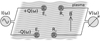 |
Fig. 1 Schematic drawing of the electric antenna configuration used in a typical quadrupolar mutual impedance experiment. The emitter antenna (E1-E2) is connected to the current generator, while the receiver antenna (R1-R2) is connected to the voltage measurement. |
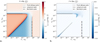 |
Fig. 2 Symmetric logarithmic representation of the real, panel a, and imaginary, panel b, part of the function |

3 Electrostatic hypothesis for mutual impedance experiments in magnetized plasma
The objective of this section is to justify the electrostatic hypothesis made in Sect. 2 by showing that the receiving antenna of a mutual impedance experiment is more sensitive to electrostatic waves than to electromagnetic ones. As a result, the main contribution to the mutual impedance spectrum is to be attributed to electrostatic waves. In this section, we focus on the magnetized regime, fpe/fce ~ 1. To discuss the sensitivity of mutual impedance experiments, we underline that a dipolar antenna is most sensitive to waves with a wavelength comparable to the antenna length. For a dipolar antenna formed by two spherical sensors, the antenna typical length scale is the separation between the two electrodes.
Waves propagating in a magnetized plasma close to the plasma frequency are shown in Fig. 3 in the form of dispersion surfaces, obtained using the numerical linearized Vlasov- Maxwell solver WHAMP, for a homogeneous, magnetized, and Maxwellian plasma (Roennmark 1982). The dispersion relation is presented in three-dimensional space, f, k⊥, k‖, as surfaces, f = f (k⊥, k‖), where the perpendicular and parallel direction are defined with respect to the mean ambient magnetic field. The frequency, f, is normalized to the plasma frequency, and the wave numbers, k⊥ and k‖, are normalized to the Debye length. The different dispersion surfaces, shown with different colors in Fig. 3, are listed in order of increasing frequency with the nomenclature used by Andre (1985):
The fast magnetosonic surface (blue) is located at frequencies lower than the electron cyclotron frequency. This mode is the high-wave-number extension of the fast magnetosonic branch – in the specific case of parallel propagation that of the whistler mode – that undergoes the cutoff at the electron cyclotron frequency. These modes become electrostatic for large enough k. This behavior is shown in the left panel of Fig. 4, in which we show the normalized difference between the frequency for the fast magnetosonic dispersion surface obtained in the general electromagnetic case by WHAMP (as in Fig. 3) and by solving in the electrostatic limit; namely,
 , Eq. (3). This difference is small if the mode becomes electrostatic, as is shown in the large k part of the left panel of Fig. 4. This dispersion surface is responsible for the generation of the low part of the interference cone structure discussed in Appendix B and presented in Fig. B.7.
The upper-hybrid surface (orange) is located around the upper-hybrid frequency. The upper-hybrid dispersion surface is electromagnetic in the low wave number limit, and is usually referred to as the Z-mode. For higher wave numbers, the dispersion surface becomes electrostatic. This behavior is shown, as for the fast magnetosonic dispersion surface, in the right panel of Fig. 4, where the difference between the electromagnetic and electrostatic solutions of the dispersion relation becomes small as k ⋅ λDe becomes larger than, approximately, 10−3. In the limit of parallel propagation, the upper-hybrid surface is the high k part of the Langmuir mode. In the limit of perpendicular propagation, it is the branch of the Bernstein modes that crosses the plasma frequency.
The L-O surface (green) is located above the plasma frequency. For large-enough wave numbers, it is electromagnetic, and it represents: for parallel propagation, the left circularly polarized ordinary mode (L mode), and for perpendicular propagation, the ordinary mode (O mode). In the case of parallel propagation, it represents the low wave number part of the Langmuir dispersion relation. The transition between the Langmuir mode and L mode is at approximately
 (Graham et al. 2018), where c is the speed of light. For higher frequencies, this dispersion surface represents the electromagnetic dispersion relation,
  .
.The R-X dispersion surface (violet) is located above the plasma frequency, is electromagnetic, and represents: for parallel propagation, the right circularly polarized mode (R mode), and for perpendicular propagation, the extraordinary mode (X mode). It has the same limit as the L-O surface for high frequency.
On top of those, we present the (electron) Bernstein waves propagating perpendicular to the magnetic field as black lines in Fig. 3. Each of these waves has a small electromagnetic component (Krall & Trivelpiece 1973, Sect. 8.12 therein) that is negligible for the sake of our instrumental model. Among the Bernstein branches, the one that belongs to the upper-hybrid surface presents in addition an electromagnetic part for small k, where this wave is the Z-mode.
To justify the electrostatic approximation adopted to model our experimental setup, we discuss how the plasma modes located in the electromagnetic parts of these dispersion surfaces are expected to be negligible compared to the ones located in the electrostatic parts. We assume here that the same amount of energy from the emitting antenna of the mutual impedance experiment is deposited in electrostatic and electromagnetic modes. We organize the following discussion by analyzing different frequency regions; namely, f ≳ fpe, f ≫ fpe and f ≲ fpe, f ≪ fpe.
First, we considered a frequency that is larger but comparable to the plasma frequency, f ≳ fpe. In this region, two modes are present: the electrostatic modes belonging to the high k part of the upper-hybrid surface and the electromagnetic modes associated with the L-O and R-X surfaces. We considered as an example f = 1.1 fpe .In the case of the plasma parameters considered in Fig. 3, the wavelength of the electrostatic modes is in the range of λe.s. ϵ (6,26) ⋅ λDe, while the wavelength of the electromagnetic modes is in the range of λe.m. ϵ (4300,6000) ⋅ λDe. Therefore, the wavelength of the electromagnetic modes is much larger than the one of the electrostatic modes, λe.m. ≫ λe.s.. From an instrumental point of view, this means that – for oscillations at a given electric energy – the signal measured by a dipolar antenna characterized by dimensions much smaller than these wavelengths will be dominated by that of the electrostatic modes. We therefore conclude that the electrostatic modes associated with the upper-hybrid dispersion surface are dominant and that the other, electromagnetic modes can indeed be neglected.
Second, we considered a frequency that is much larger than the plasma frequency, f ≫ fpe. In this frequency region, only the electromagnetic modes of the L-O and R-X dispersion surfaces are present. The wavelength associated with these modes decreases for increasing frequency. Therefore, to consider a minimum value of the wavelength associated with these modes, we took an upper value for the frequency investigated by a mutual impedance experiment of f = 25 ⋅ fpe. In this case, the characteristic wavelength of the L-O and R-X dispersion surfaces is 130 ⋅ λDe. This value is much larger than the one of the electrostatic modes considered previously, λe.s. ϵ (6,26) ⋅ λDe, and is therefore also considered as negligible. We also wish to highlight that the plasma mode associated with the high-frequency range of the L-O and R-X dispersion relation is the same as in the absence of a magnetic field, or even in vacuum. This means that: (i) this mode would have been already observed, if present, by previous mutual impedance experiments, and (ii) it will be removed by the normalization of the mutual impedance spectrum to its value in vacuum.
Third, we considered a frequency that is smaller but comparable to the plasma frequency, f ≲ fpe. In this case, the only mode is the electromagnetic part of the upper-hybrid dispersion relation; namely, the Z-mode. For the plasma parameters of Fig. 3, the wavelength associated with this mode is larger than 3000 ⋅ λDe, making it therefore negligible compared to the electrostatic modes, as was previously discussed.
Fourth, we considered a frequency that is much smaller than the plasma frequency, f ≪ fpe .In this case, we must consider the high-wave-number extension of the fast magnetosonic mode. It is composed of an electrostatic part for wavelengths on the order of 10 ⋅ λDe and of an electromagnetic part for wavelengths on the order of 1000 ⋅ λDe. As for the upper-hybrid surface, we therefore state that only the electrostatic part can be observed by the experimental setup. This claim is substantiated by the fact that the interference cone structure, which is produced by the fast magnetosonic dispersion surface, was successfully reproduced in the electrostatic approximation (Fisher & Gould 1971; Rohde et al. 1993).
Last, as was already discussed, the electromagnetic counterpart of electron Bernstein waves is negligible, so that these modes are considered essentially electrostatic. It must be noted that the branch that belongs to the upper-hybrid surface is not electrostatic for all wavelengths, as it becomes electromagnetic at low wave numbers. This limit case is included in the discussion, presented in this section, regarding the upper-hybrid dispersion surface.
In the next section, we focus on the results obtained from the new mutual impedance model in magnetized plasmas.
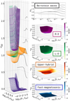 |
Fig. 3 Dispersion surfaces obtained with the numerical linearized Vlasov-Maxwell solver WHAMP, for a homogeneous, magnetized, and Maxwellian plasma (Roennmark 1982), for ne = 1.4 cm−3, Te = 2 eV, B = 132 nT, (fpe/fce = 2.88) presented all together (left) and separately, with color indicating the ratio of the magnetic to electric field (right) on a logarithmic scale. The frequency is normalized to electron plasma frequency, and the wave numbers, presented on a logarithmic scale, to the Debye length. |
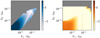 |
Fig. 4 In color, we present log10 |(fWHAMP − fe.s.)/fWHAMP|, where fWHAMP is the frequency obtained by the WHAMP (Roennmark 1982) solver in the general electromagnetic case, and fe.s. is the frequency obtained by solving the dispersion relation |

4 Effects of magnetic field strength and direction on mutual impedance measurement
In this section, we explore the expected response of mutual impedance experiment in a magnetized plasma. Eq. (6) is solved numerically (see Appendix A) and used to produce mutual impedance spectra for different plasma parameters and magnetic field values. Furthermore, we assess the efficiency of mutual impedance experiments as a plasma diagnostic.
The analysis of these numerical spectra provides an insight into how to obtain a plasma diagnostic from mutual impedance experiments in a magnetized plasma. The charge distribution on the emitting antenna is a point-like one, according to one of the hypotheses detailed in Sect. 2. We considered two different antenna configurations. In the first configuration, we used two monopolar electric antennas, one for reception and one for emission (see Sect. 4.1). In the second configuration, we used two dipole antennas (for a total of four electrodes), one for reception and one for emission (see Sect. 4.2). We produced synthetic numerical spectra for both configurations. In this section, we focus on the amplitude of the computed mutual impedance spectra; the phase spectra are briefly discussed in Appendix C.
4.1 Monopole antenna
We considered as our first example of mutual impedance spectra the case of a monopolar antenna. Multiple mutual impedance spectra are presented in Fig. 5, organized so that the electron temperature increases from bottom to top, while the magnetic field increases from left to right. In each plot, three different directions of the instrument sensors (i.e., emittingreceiving direction) with respect to the background magnetic field are considered, from quasi-parallel (dotted green) to oblique (dashed red) and quasi-perpendicular (solid blue). These synthetic mutual impedance spectra illustrate how the magnetic field direction and strength influence the shape and location of the maximum of mutual impedance spectra, from a cold (bottom panels) to a hot (top panels) plasma.
In the limit of an antenna direction quasi-perpendicular to the magnetic field, θ = 90°, shown in blue in Fig. 5, multiple local maxima and minima are present. The series of local maxima correspond to the frequencies, fqn, defined as the frequencies at which electron Bernstein waves have zero group velocity (see Sect. 1). This behavior is consistent with what was observed experimentally in the Earth magnetosphere by the mutual impedance instruments on board the GEOS-1 spacecraft (Christiansen et al. 1978), and on board the Rosetta mission during the Earth flybys (Béghin et al. 2017). Notably, the same behavior was observed by the magnetospheric electric sounder experiment WHISPER, on board the CLUSTER mission (Trotignon et al. 2001). The amplitude of these local maxima decreases as the magnetic field direction departs from a direction perpendicular to the emission-reception direction. This behavior is explained by the strong Landau damping of electron Bernstein modes when propagating not perpendicular to the ambient magnetic field. The absolute maximum of the mutual impedance spectrum is located at different characteristic frequencies depending on the value of the ratio fpe / fce.
In the regime of low magnetization, fpe /fce ≥ 2, the absolute maximum is located at the plasma frequency. In this case, the upper-hybrid frequency tends to the plasma frequency as the magnetic field strength tends to zero.
In the intermediate magnetization regime of 0.5 ≤ fpe/fce ≤ 1, the absolute maximum is located at the upper-hybrid frequency. In the particular case of fpe close to fuh (i.e., fpe/ fce ≃ 1 in Fig. 5), our model shows that a maximum is visible at the upper hybrid frequency, while no local maximum is seen at the plasma frequency. This (modeling) result is consistent and explains the (experimental) results obtained by Pottelette et al. (1981) and Decreau-Prior (1983) in a similar regime that also did not observe a resonance at the plasma frequency, but at the upper hybrid frequency instead, with the measurements performed by the mutual impedance experiments on board the Porcupine sounding rocket in the Earth ionosphere and GEOS satellite in the Earth magnetosphere, respectively. With a slightly higher magnetic field, such that fpe/fce ≃ 0.5, a local maxima at the plasma frequency might be observed depending on the electron temperature and the magnetic field direction, with an amplitude smaller than the resonance at the upper hybrid frequency.
In the high magnetization regime, fpe /fce ≤ 0.2, the maxima located at the plasma frequency and at the upper-hybrid frequency are of similar amplitude, meaning that the absolute maximum corresponds to one or the other depending on the magnetic field orientation. The amplitude of the maximum at the upper-hybrid frequency increases as the electron temperature decreases. This effect is analogous to what happens in the unmagnetized case to the maximum at the plasma frequency (Gilet 2019, Fig. 4.3 therein). The same behavior is observed for the secondary maxima at the fqn frequencies.
The monopole antenna configuration is to be considered as a unitary test: it is the simplest configuration possible, and it is extremely useful to understand how the signal propagates, but it is not actually used in practice for space flight mutual impedance experiments. A dipolar antena configuration is instead typically preferred as it enables some of the electromagnetic noise originating from the spacecraft platform to be reduced. In the following section, we present the mutual impedance spectra computed for one representative example of dipolar antennas.
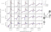 |
Fig. 5 Mutual impedance spectrum for a monopolar antenna emission and reception, according to the geometry presented in the figure. The parameters used for this calculation are: from left to right, fpe/ fce = 5, 2, 1, 0.5, 0.2, and from bottom to top, λDe = 5, 10, 20, 40 cm. The different curves correspond to a different angle between the magnetic field and the emission-reception direction. |
4.2 Dipole antenna
In this section, we consider mutual impedance spectra computed for one representative example of quadrupolar antenna configuration: dipolar both in emission and in reception. In this case, the normalized mutual impedance spectrum is computed as
 (7)
(7)
where V/V0 is defined in Eq. (6), and xr1, xr2 (resp. xe1, xe2) are the positions of the receiving (resp. emitting) electrodes (see Fig. 1).
We considered here a quadrupolar antenna configuration similar to that of the RPC-MIP instrument on board the Rosetta spacecraft (Trotignon et al. 2007). The sensor’s geometry and the mutual impedance spectra computed in this configuration are both shown on Fig. 6. The validation of the numerical calculation in the unmagnetized limit, shown in Fig. B.6, was performed with the same geometry.
The antenna(s)’s geometry significantly influences the instrumental response of mutual impedance experiments, in particular the shape and the amplitude of the mutual impedance spectrum. This is illustrated by the comparison between the mutual impedance spectra expected for the two considered antenna geometries – namely, monopole and dipole – shown on Figs. 5 and 6, respectively. When comparing these two figures, the reader will notice that the amplitude scales are different, while all the other parameters – the frequencies, the typical antenna distances, the magnetic field angle, and the set of plasma parameters, fpe / fce and λDe - have been kept identical. The use of a dipolar antenna (Fig. 6) can in some cases smooth the resonances.
The characteristic frequencies observed in these mutual impedance spectra are the same as those detailed in Sect. 4.1; namely, the Bernstein frequencies, fqn, the upper-hybrid frequency, fuh, and the plasma frequency, fpe. For low magnetization – fpe /fce ≥ 0.5 – the absolute maximum is still found at the upper-hybrid frequency. For all values of fpe / fce that are presented, an increased electron temperature still results in a lower amplitude of the mutual impedance spectrum. Notably, the prominence of the maxima at the fqn frequencies depends upon the electron temperature. This results in the fact that the maxima at the fqn frequencies are not always more prominent in the case of perpendicular propagation. Such behavior is inferred by comparing the results from the first and last line of Fig. 6: the fqn maxima are more prominent in the case of a perpendicular in the bottom row (small Debye length) and more prominent in the case of a parallel antenna in the top row (large Debye length).
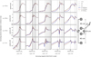 |
Fig. 6 Mutual impedance spectrum for a quadrupolar configuration, according to the geometry presented in the figure, and compatible with the one of the RPC-MIP instrument on board the Rosetta spacecraft. The parameters used for this calculation are the same used in Fig. 5. |
4.3 Plasma diagnostic from magnetized mutual impedance spectra
One method of obtaining a plasma diagnostic from mutual impedance experiments is to find the best fit between the measured spectra and a numerical model (Wattieaux et al. 2020), as a function of the plasma parameters. Another method is to analyze specific features of the spectrum, related directly to the plasma parameters (Chasseriaux et al. 1972), such as, in the unmagnetized case, the maximum and phase change at the plasma frequency (to retrieve the plasma density), and the minimum next to the plasma frequency (related to the Debye length). In the following, we list a number of features of magnetized mutual impedance spectra that can be used as a plasma diagnostic. We organize this discussion with different magnetization levels, meaning different ranges of the ratio fpe/ fce.
We start by observing that, if the magnetization is low enough, fpe /fce ≥ 5, the magnetized mutual impedance spectrum is well described by the unmagnetized mutual impedance spectrum, with additional local maxima at the fqn frequencies superposed on it. This means that, in this case, the upper-hybrid frequency, fuh, is retrieved by the absolute maximum of the spectrum or by the inflexion point of the spectrum, depending on the electron temperature (see Fig. 6). The magnetic field is more easily derived by considering the low-frequency part of the spectrum, where local minima or maxima (depending on the antenna geometry) are present close to the multiple of the electron cyclotron frequency, fce. In this regime, it is possible to derive the electron temperature from the amplitude of the maximum at the upper-hybrid frequency, as is done in Gilet (2019), as it does not depend significantly on the direction of the magnetic field.
In the case of fpe /fce ≃ 1, the absolute maximum of the mutual impedance spectrum is located at the upper-hybrid frequency if the Debye length is small enough, λDe < 20 cm. This maximum was used to retrieve the plasma density. The maxima at the fqn frequencies are visible. From those, it is possible to derive the ratio of plasma-to-electron cyclotron frequencies with the help of Hamelin’s diagram (Pottelette et al. 1981), presented in Fig. 7. This diagram shows the differences, fqn – n · fce , normalized to fce, presented as a function of fpe /fce, where n is the order of the Bernstein wave frequency band (here, n is chosen from 1 to 8). Once the magnetic field is known and the fqn frequencies are identified from the mutual impedance spectrum, one should represent such frequencies on the Hamelin’s diagram. The alignment of those frequencies to the theoretical curves shown in Fig. 7 gives an estimate of the ratio, fpe / fce. An example of such a use of Hamelin’s diagram is presented in Fig. 4 of Trotignon et al. (2001).
Considering the regime of strongly magnetized plasma, fpe/fce ≤ 0.2, the maxima at the plasma frequency and at the upper-hybrid frequency are both identifiable. From them, both the plasma density and the amplitude of the magnetic field are derived. We note that the plot for λDe = 40 cm and fpe / fce = 0.2 (upper right) in Fig. 6 corresponds to a regime in which λDe ≃ d and  , with d the size of the dipo-lar antenna. This means that in the case of strongly magnetized plasma, even if the Debye length is comparable to the size of the antenna, multiple resonances are visible. Still, the amplitude of these resonances decreases with increasing temperature.
In this section, we have focused on an isotropic, collisionless magnetized plasma. In the next two sections, we consider two other cases; namely, the case of a magnetized plasma with electron temperature anisotropy and the case of a plasma with presence of electron-neutral collisions. We start with the case of an anisotropic plasma.
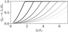 |
Fig. 7 Hamelin’s diagram, which presents |

5 Effect of temperature anisotropy on magnetized mutual impedance experiments
In the previous section, we have focused on an isotropic magnetized plasma. However, past measurements in space plasmas have shown that electron temperature anisotropies are frequently observed. For instance, parallel temperature anisotropies are known to be generated in the electron foreshock upstream quasiparallel shocks (Chisham et al. 1996) and in the cusps of magnetized planets (Demars & Schunk 1987), and perpendicular temperature anisotropies are known to be generated downstream of quasi-perpendicular shocks (Montgomery et al. 1970). Forthcoming space missions carrying mutual impedance experiments such as BepiColombo and JUICE are likely to encounter plasmas with some level of electron temperature anisotropy. We therefore investigate in this section whether – and in which cases – mutual impedance measurements can provide a diagnostic of electron temperature anisotropies in magnetized space plasma. For this reason, we next considered an electron temperature anisotropy Te,⊥ /Te,|| ≠ 1.
For this purpose, we first remind ourselves of the range of temperature anisotropy that is expected in a magnetized plasma, then we compute and discuss the corresponding expected mutual impedance spectra, and we finally discuss the dependency of the mutual impedance spectrum features on the electron temperature anisotropy. In this section, we consider a bi-Maxwellian electron distribution characterized by two temperatures, Te,⊥ and Te,||, which results in the dielectric function presented in Eq. (5). All other hypotheses are identical to the ones used previously and detailed in Sect. 2.
First, we must recall the expected range of temperature anisotropies in stable space plasmas; that is, ones for which no plasma instability is triggered. The two instabilities that constrain a bi-Maxwellian plasma are electromagnetic in nature and are: the whistler instability, Te,⊥/Te,|| > 1, and the oblique fire hose instability, Te,⊥ /Te,∣ < 1 (Stverák et al. 2008, Fig. 5 therein). Their analytical approximations are presented, for example, in Gary & Cairns (1999), Gary & Nishimura (2003), and Gary & Karimabadi (2006), and are reproduced here in Fig. 8. The model developed in this work is electrostatic, and therefore blind to these instabilities. In other words, these (electromagnetic) instabilities are not described in our (electrostatic) model. Therefore, we limited our (electrostatic) calculation to a temperature anisotropy range that is stable to such (electromagnetic) instabilities. This (stable) electron temperature anisotropy range is shown in Fig. 8, where the electron temperature anisotropy stability limits for the whistler and fire-hose instabilities are presented as a function of both the electron plasma beta. We also indicate in the top axis the corresponding electron parallel temperature in the case of fpe / fce = 5. We started by considering the case of Te,⊥ /Te,|| < 1, where the stable temperature anisotropy domain is bound by the oblique fire-hose instability. The expected electron temperature for the space plasmas explored by mutual impedance experiments varies in the range of (10–2, 10+3) eV, corresponding to 10–4 ≤ vth.e /c ≤ 5 ⋅ 10–2. Given that  , for all the temperatures considered: βe,|| < 10–1, as is presented in Fig. 8. Therefore, the ratio Te,⊥/Te,|| can get as low as 10–2 in a stable plasma. We then considered the case of Te,⊥ /Te,|| > 1, where the stable temperature anisotropy domain is bound by the whistler instability. From the analytical limits presented in Fig. 8, we see that if Te,|| ~ 10 eV it is possible to observe temperature anisotropies as high as Te,⊥ /Te,|| ~ 10. We therefore consider in the rest of our study an electron temperature anisotropy range of 10–2 ≤ Te,|| / Te,⊥ ≤ 10+1.
Second, we have computed the mutual impedance spectra in the case of a plasma presenting an electron temperature anisotropy considering the same antenna geometries as those previously considered in Sect. 4.1 (resp. Sect. 4.2) in Fig. 9 (resp. Fig. 10). Here, we consider a fixed value of fpe/fce = 1.4, in order to better distinguish the plasma frequency and the harmonics of the electron cyclotron frequency.
The spectra presented in Figs. 9 and 10 show that for a lower (resp. higher) value of the temperature anisotropy, Te,⊥/Te,||, the local maxima at the fqn frequency are less (resp. more) pronounced. To highlight this behavior, we show in Fig. 11 the amplitude of the first (resp. second) local maximum at the fq1 (resp. fq2) frequencies as a function of the angle between the magnetic field and the emission-reception direction, for the monopole geometry (Fig. 9).
To interpret this behavior, we present in Fig. 12 the temporal damping rate, ℑ(f /fce), for the branch of Bernstein waves with 3 ⋅ fce ≤ f ≤ 4 ⋅ fce , obtained numerically (Roennmark 1982) with fpe/fce = 1.4. This branch was chosen as it is the first branch with f > fuh, meaning that it produces the local maximum in the mutual impedance spectrum closest to the upper-hybrid frequency, which is the most prominent one. The cone in which the Bernstein mode can propagate increases as the perpendicular temperature increases (Fig. 12). Therefore, the local amplitude maxima in the mutual impedance spectra at the fqn frequencies are more prominent as the perpendicular temperature increases, as is shown in Figs. 9 and 10. Notably, this is the opposite of the behavior that we described, in an isotropic magnetized Maxwellian plasma, for the maximum amplitude at the upper-hybrid frequency, which instead decreases as the electron temperature increases, as is shown in Figs. 5 and 6.
We argue that it will be possible to diagnose an electron temperature anisotropy with a mutual impedance experiment, and we consider two possible approaches to doing so, as is done in Sect. 4.3. First, the shape of the mutual impedance spectrum changes depending on the electron temperature anisotropy. This means that a best fit between the mutual impedance numerical model and the measurements could include the temperature anisotropy as a free parameter. Second, the relative amplitude of the maxima at the fqn frequencies and the upper-hybrid frequency changes depending on the temperature anisotropy, providing an even more straightforward diagnostic based on the analysis of only a few features in the mutual impedance spectrum.
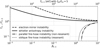 |
Fig. 8 Analytical limits of different plasma instabilities generated by an electron temperature anisotropy; in particular, the electron mirror instability (Gary & Karimabadi 2006) (γ/ωce = 0.001), the whistler instability (Gary & Karimabadi 2006) (γ/ωce = 0.001), and the parallel and oblique fire-hose instability (Gary & Nishimura 2003) (γ/ωce = 0.01). |
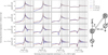 |
Fig. 9 Mutual impedance spectrum for a monopolar antenna configuration, as in Fig. 5, according to the geometry presented in the figure. Here, the ratio of plasma to electron cyclotron frequency is fpe/ fce = 1.4, as in Fig. 13. The electron temperature anisotropy, Te,⊥/Te,||, is presented on the horizontal axis increasing from left to right, and is considered in the model by the use of Eq. (5). |
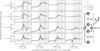 |
Fig. 10 Mutual impedance spectrum for a quadrupolar antenna compatible with the one of the RPC-MIP instrument, as in Fig. 6, with different electron temperature anisotropy, as in Fig. 9. |
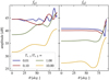 |
Fig. 11 Amplitude of the maxima at the first two fqn frequencies as a function of the angle between the magnetic field and the antenna emission-reception direction, for a monopolar geometry such as the one presented in Fig. 9. The amplitude increases as the angle approaches 90 degrees. |
6 Effects of electron-neutral scattering on magnetized mutual impedance experiments
In previous sections, we have focused on a collisionless plasma. In this section, we now consider the case of a plasma in which electron-neutral scattering is present. The effects of electronneutral collisions are relevant for studies of the Earth’s ionosphere (Spencer & Patra 2015) and cometary and planetary ionospheres where the collisional coupling with the neutral atmosphere is significant (Yamauchi et al. 2022). Such electronneutral collisional regions are of significant scientific interest, as is shown by the Daedalus mission project (Sarris et al. 2020), designed to probe for the first time this region that collisionally couples the lower ionosphere with the upper atmosphere of the Earth. A mutual impedance experiment is suggested to be part of the Daedalus instrumental payload (Sarris et al. 2020). The preliminary orbits defined for this mission would explore the low ionosphere in the region between 100 km and 200 km of altitude. There, the ratio between the electron-neutral scattering frequency and the plasma frequency is estimated to reach values as large as fne/ fpe = 10–4 (Pfaff 2012; Bernhardt et al. 2009). Using the model described in this work, we take into consideration both the effects of the Earth’s magnetic field and of electron-neutral collisions on mutual impedance measurements.
Numerical mutual impedance spectra are presented in Fig. 13, for different values of the electron-neutral collisional frequency (horizontal axis) and Debye length (vertical axis). Multiple spectra are presented, each corresponding to a different angle between the antenna and the magnetic field. The main consequence of the presence of electron-neutral scattering is that the overall spectrum is smoothed, and the maxima of the mutual impedance spectrum become less pronounced. Our results show that the mutual impedance experiments are not sensible to the electron-neutral scattering for values of fne / fpe < 10–3. Therefore, from an instrumental perspective, the plasma is to be considered collisionless for fne /fpe < 10–3.
7 Conclusions
The primary objective of this work is to investigate whether a quantitative plasma diagnostic (density, temperature) can be provided by mutual impedance experiments in magnetized space plasmas. A secondary objective is to explore the possibility of measuring electron temperature anisotropies with mutual impedance experiments.
To achieve the objectives of this work, we developed the first quantitative instrumental model for mutual impedance experiments in a magnetized plasma; namely, a model for the computation of the mutual impedance spectrum, Z (f) = Z (f, ne, Te,⊥, Te,||, B). Our model is valid for arbitrary values of the plasma density and electron temperature, as well as for arbitrary strength and orientation of the magnetic field. We considered three different plasma conditions: (i) an isotropic magnetized Maxwellian electron distribution in a collisionless case, (ii) a magnetized Maxwellian electron distribution with temperature anisotropy in a collisionless case, and (iii) an isotropic magnetized Maxwellian electron distribution with electron-neutral scattering.
We note that the generic model developed in this work actually represents the Green function of the instrumental response in a magnetized plasma. As such, it can be used for different mutual impedance experiments, characterized by different spatial configurations of the electric sensors and of the nearby conductive spacecraft.
From the results of our model, we identified the characteristic frequencies corresponding to local maxima in the mutual impedance spectrum. These frequencies are the upper-hybrid frequency, the plasma frequency, and the so-called fqn frequencies. From the characteristic frequencies of the mutual impedance maxima, it is possible to directly extract a diagnostic for the plasma density and magnetic field strength.
We identified different magnetization regimes, depending on the ratio fpe / fce. In the low magnetization case, fpe /fce >> 1, the mutual impedance spectrum shows an absolute maximum at the plasma frequency (equal to the upper hybrid frequency in this regime), with an envelope similar to the spectrum computed in an unmagnetized plasma over which local maxima are present at the fqn. In the intermediate magnetization case, fpe /fce ≃ 1, the absolute maximum of the mutual impedance spectrum is located at the upper-hybrid frequency, with local maxima at the fqn frequencies, while the plasma frequency does not show any notable resonance. In the strong magnetization case, fpe / fce << 1, local maxima are present at the plasma and upper-hybrid frequency, as well as at the fqn frequencies. The magnetic field therefore has two main effects on the mutual impedance spectrum: first, it separates the plasma frequency from the upper-hybrid frequency, making them distinguishable, and second, it produces maxima at the fqn frequencies that become more pronounced the stronger the magnetic field.
The magnetic field direction significantly influences the amplitude of these local maxima; in particular, those corresponding to the fqn frequencies. For a Debye length that is smaller than the distance between the mutual impedance antennas, the fqn maxima become more pronounced the closer the antenna is to the direction perpendicular to the magnetic field. This is compatible with the fact that Bernstein waves propagate essentially perpendicular to the magnetic field. However, and interestingly, for a Debye length that is not smaller than the distance between the mutual impedance antennas, the fqn maxima can also be observed for other directions of propagation. Practically, the mutual impedance spectra expected in a magnetized plasma is strongly dependent on the geometry of the sensors. Therefore, the modeling effort performed in this work is essential to the analysis of mutual impedance data.
In this work, we also relaxed the hypothesis of a collisionless plasma by adding electron-neutral scattering to our instrumental model. We did this for two purposes. The first purpose is to provide a regularization method for our numerical calculation that carries some physical meaning, and that can be used to check the validity of a purely numerical regularization method. The two regularization techniques are robust, as they indeed produce the same results. The second purpose is to explore the effects of electron-neutral scattering on mutual impedance experiments, with applications for Earth, cometary, and planetary ionospheric space missions. From this model, we derived that the main effect of electron-neutral scattering is to smooth the mutual impedance spectrum. We also inferred that for a ratio of electron-neutral scattering frequency to plasma frequency, fne / fpe < 10–3, mutual impedance experiments are not sensitive to scattering effects, which also defines the regime for which the plasma is to be considered collisionless from an instrumental perspective.
The mean amplitude of the mutual impedance spectrum decreases with increasing electron temperatures, as is the case in the unmagnetized regime. This behavior carries over to the case of a Debye length that is comparable to the distance between emitting and receiving antennas. The amplitude of the local maxima of the mutual impedance spectrum follows the same behavior as a function of the electron temperature, and therefore could be used as a direct and simple diagnostic of the electron temperature.
In the case of a collisionless magnetized plasma, the electron temperature can be anisotropic, Te,⊥ , Te,||, while the plasma remains stable. In the electron temperature anisotropy range that preserves stability, we found a significant effect of the electron temperature anisotropy on mutual impedance measurements. We showed that it controls the spectral amplitude at the fqn frequency. This is consistent with the fact that, as Te,⊥/Te,|| increases, the cone of propagation of Bernstein waves also increases. We therefore argue that electron temperature anisotropies could be diagnosed with mutual impedance experiments. This novelty will open new possibilities to investigate the electron temperature anisotropies generation and relaxation in space plasma, as mutual impedance spectra can be performed at high cadences. The sensitivity to electron temperature anisotropy is highly dependent on the sensor geometry, as well as on the interaction between the experiment and the (conductive) spacecraft geometry. A proper uncertainty analysis deserves to be carried out for the specific cases of the PWI/AM2P (resp. RPWI/MIME) mutual impedance experiment of the Bepi- Colombo (resp. JUICE) planetary mission, but this endeavor remains out of the scope of this present work.
Before concluding, we wish to highlight one limitation of our approach. In this work, we do not take into consideration the presence of a plasma sheath around the sensors or the spacecraft. The plasma sheath influences the response of mutual impedance if the sheath dimension, which scales as the Debye length, is of the order of the inter-sensor distance, and has an effect on the evaluation of the electron temperature from mutual impedance experiments. The influence of the plasma sheath on mutual impedance experiments has been investigated in the unmagnetized plasma case with different approaches (Wattieaux et al. 2019; Bucciantini et al. 2023b). A similar study in the magnetized plasma case would be beneficial in the future. For this purpose, the numerical calculation presented here is ready to be coupled with techniques accounting for a realistic spacecraft and antenna geometry (Wattieaux et al. 2019), including the plasma sheath.
Our instrumental model will enable one to properly model the BepiColombo PWI/AM2P and Juice RPWI/MIME mutual impedance experiments that will perform measurements of the electron properties around Mercury and in the Jupiter system, respectively. A first interesting opportunity to test this new model is the first Earth flyby of JUICE planned in summer 2024.
 |
Fig. 12 Temporal damping rate, ℑ(f /fce), for the branch of Bernstein waves with 2 ⋅ fce ≤ f ≤ 3 ⋅ fce, presented as a function of the perpendicular (resp. parallel) wave number, k⊥ (resp. k||). The wave numbers are normalized relative to the parallel Larmor radius, rLe,|| = Tth,e,||/ωce, and fpe/fce = 1.4. Lines of a constant angle with the magnetic field are also presented. These results were obtained with the numerical linearized Vlasov-Maxwell solver WHAMP, for a homogeneous, magnetized, and Maxwellian plasma (Roennmark 1982). |
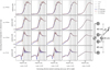 |
Fig. 13 Mutual impedance spectrum for a quadrupolar configuration, according to the geometry presented in the figure, and compatible with the one of the RPC-MIP instrument on board the Rosetta spacecraft. Here, the ratio of plasma to electron cyclotron frequency is fpe/fce = 1.4. The effect of electron-neutral scattering, modeled by Eq. (4), is presented by the decreasing electron-neutral collision frequency on the horizontal axis, from left to right. |
Acknowledgements
The authors acknowledge support from the Federation CaSciModOT (CCSC Orleans-Tours, France) for access to the Region Centre computing cluster.
Appendix A Numerical solution to the mutual impedance model in a magnetized plasma
This appendix describes the computation of the electric potential derived in Eq. (6). For our numerical computation, we normalize the physical space to the Debye length, r, z → r/λDe, z/λDe, the wave numbers to the inverse of the Debye length, kr , kz → kr λDe , kzλDe , the frequency to the plasma frequency, f → f / fpe . The thermal velocity is chosen so that vth,e = ωpeλDe. In the case of electron temperature anisotropy, we use instead λDe,|| .
The numerical integration of Eq. (6) is performed in the wave vector domain ![Mathematical equation: ${k_r} \in \left[ {k_r^{\min .},k_r^{\max .}} \right]$](/articles/aa/full_html/2025/04/aa50312-24/aa50312-24-eq32.png) and
and ![Mathematical equation: ${k_z} \in \left[ {k_z^{\min },k_z^{\max .}} \right]$](/articles/aa/full_html/2025/04/aa50312-24/aa50312-24-eq33.png) , as justified in appendix B. To improve the numerical efficiency, it is convenient to actually compute a reformulated and equivalent version of Eq. (6), that reads:
, as justified in appendix B. To improve the numerical efficiency, it is convenient to actually compute a reformulated and equivalent version of Eq. (6), that reads:
![Mathematical equation: $\eqalign{ & {V \over {{V_0}}}(r,,\omega ) = {e^{ - {{\sqrt {{r^2} + {^2}} } \over {{\lambda _{{D_e}}}}}}} + {{2\sqrt {{r^2} + {^2}} } \over \pi }\int_{k_r^{{\rm{min}}{\rm{. }}}}^{k_r^{{\rm{max}}{\rm{. }}}} d {k_r}\int_{k_^{{\rm{min}}{\rm{. }}}}^{k_^{{\rm{max}}{\rm{. }}}} d {k_} \cr & {{{k_r}{J_0}\left( {{k_r}r} \right)\cos \left( {{k_}} \right)} \over {k_r^2 + k_^2}}\left[ {{1 \over {{\varepsilon _L}\left( {{k_r},{k_},\omega } \right)}} - {1 \over {\varepsilon _L^\infty (k)}}} \right]\delta \left( {\omega - {\omega _e}} \right) \cr} $](/articles/aa/full_html/2025/04/aa50312-24/aa50312-24-eq34.png) (A.1)
(A.1)
where:
 (A.2)
(A.2)
and
 (A.3)
(A.3)
The numerical integration is performed using an adaptive integration scheme organized as follows. First, the integrand function is computed on a rectangular logarithmic coarse grain grid. Second, the grid is split into four rectangular coarse grain sub-grids. Third, the integral is computed on each of these subgrids for a fixed spatial position r, z. Fourth, points are added to each of these sub-grids, generating new finer sub-grids. This is done by adding the middle points to the original grid. The integrand function is computed again on the newly added grid points. These four new sub-grids are used for the computation of the integral, for a fixed spatial position r, z. Convergence is reached if, on each of these subdivisions, the difference between the integral computed using the coarse and the fine sub-grid is less than a set constant, δabs. . This procedure provides a grid for the numerical integration that tends to accumulate points around the singularities of the integrand function. The structure of the consecutive subdivisions operated by this integration scheme is presented in Fig. A.1. The values of the integrand computed on the adaptive grid are reused to compute the integral at different spatial positions, meaning for different values of r, z. This numerical scheme has been validated in successive steps, as discussed in detail in appendix B. This calculation provides the function V/ V0 as a function of spatial position r, z.
In order to avoid divisions by zero during the adaptive integration, and to limit the computation time, the integrand function in Eq. (A.1) is regularized. This can be performed by one of two techniques. The first one is purely numerical: adding a small imaginary part to the denominator εL → εL + iδdenom. The second one bares some physical meaning: including a small collision rate in the dielectric, as shown in Eq. (4). A comparison between these two regularization techniques is presented in appendix B. They provide the same result when reaching convergence.
 |
Fig. A.1 The progressively finer subdivisions produced by the numerical integration scheme is presented, using as an example one of the test functions from Genz (1984) that are used in the validation procedure described in appendix B. In the last figure, the function used in the integration is also shown in color. |
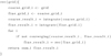 |
Fig. B.1 Pseudocode form for the numerical integration algorithm used in this work to compute the values of the potential expressed by Eq. (A.1). |
Appendix B Validation of the numerical integration scheme
In this appendix, we discuss the validation of the numerical computation of Eq. (A.1). The algorithm is described in Appendix A, and is presented in the form of pseudocode in Fig. B.1.
We start by discussing the reduction of the integration region to a limited domain, from Eq. (6) to Eq. (A.1). Eq. (6) is written in equivalent form as:
 (B.1)
(B.1)
where:
![Mathematical equation: ${\cal F}\left( {{k_r},{k_}} \right) = {{{k_r}{J_0}\left( {{k_r}r} \right)\cos \left( {{k_}} \right)} \over {k_r^2 + k_^2}}\left[ {{1 \over {{\varepsilon _L}\left( {{k_r},{k_},\omega } \right)}} - {1 \over {\varepsilon _L^\infty (k)}}} \right]$](/articles/aa/full_html/2025/04/aa50312-24/aa50312-24-eq38.png) (B.2)
(B.2)
and the integrals jj are defined over different integration domains, defined in Fig. B.2.
We now show that the integrals j3 +j6, j7 + j8, and j9 are limited, and therefore tend to zero in the limit of large  and
and  . We do this in the case
  . To do so, we start by observing that ℱ (kr, kz) ∊ ℂ and the integration is in real space, kr , kz ∈ ℝ. The imaginary part of ℱ comes from the plasma dispersion function. It is true that:
 (B.3)
(B.3)
and therefore, by using the fact that  :
:
 (B.4)
(B.4)
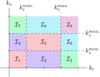 |
Fig. B.2 Illustration of the subdivision of the integration regions for the integral defined in Eq. (6), used in Eq. (B.1). |
Also:
![Mathematical equation: $\eqalign{ & \varepsilon _L^\infty \varepsilon _L^{{\rm{Max}}{\rm{. }}} = {\left( {1 + {1 \over {{k^2}\lambda _{De}^2}}} \right)^2} + \left( {1 + {1 \over {{k^2}\lambda _{De}^2}}} \right) \cr & \left[ {{1 \over {{k^2}\lambda _{De}^2}}{\omega \over {\sqrt 2 {\upsilon _{th.e}}{k_}}}\sum\limits_{n = - \infty }^{ + \infty } {{e^{ - \lambda }}} {I_n}(\lambda )Z\left( {{\xi _n}} \right)} \right] \cr} $](/articles/aa/full_html/2025/04/aa50312-24/aa50312-24-eq45.png) (B.5)
(B.5)
therefore:
 (B.6)
(B.6)
and:
 (B.7)
(B.7)
Now, by using these majorations and minoration, we majorate the real and imaginary parts of  . We first write:
 (B.8)
(B.8)
and from this:
 (B.9)
(B.9)
and the same result is valid also for  . Therefore, if one or both kr and kz tend to infinity, the behavior of
  is:
is:
 (B.10)
The contribution of j9 is proven to be negligible, meaning that:
 (B.11)
Supposing that the limit in Eq. (B.11) exists, and that ℱ(kr, kz) : ℝ2 → ℂ is continuous, implies:
 (B.12)
the hypothesis of continuity of ℱ(kr, kz) is verified in the integration region for large enough  and
and  , as to avoid any pole of the function
  , meaning any plasma eigenmode. Combining these results, and noting that
  :
:
 (B.13)
Therefore, the function ℱ (kr , kz) is dominated by the integrable function ℱdom.(kr, kz), and Lebesgue’s dominated convergence theorem applies (admitting the inversion of the integration and limit). Therefore:
 (B.14)
The contribution of both j3 +j6 and j7 +j8 is proven to be negligible, meaning that:
 (B.15)
This result is proven the same as was shown for j9 , by moving the limit inside the integral. To conclude, it is necessary to show that  even if only either kr or kz tend to infinity. This is done in the following. The expansion of the modified Bessel function, In (λ), of the first kind for large real argument, λ ∈ ℝ, is
  . Therefore:
![Mathematical equation: $\eqalign{ & {\varepsilon _L}\left( {{k_r},{k_},\omega } \right) \simeq \cr & \simeq 1 + {1 \over {k_r^2\lambda _{De}^2}}\left[ {1 + {\omega \over {\sqrt 2 {\upsilon _{th.e}}{k_}}}{1 \over {\sqrt {2\pi } }}{1 \over {{k_r}{r_{Le}}}}\sum\limits_{n = - \infty }^{ + \infty } Z \left( {{{\omega - n{\omega _{ce}}} \over {\sqrt 2 {\upsilon _{th.e}}{k_}}}} \right)} \right] \simeq \cr & \simeq 1 + {1 \over {k_r^2\lambda _{De}^2}} \cr} $](/articles/aa/full_html/2025/04/aa50312-24/aa50312-24-eq65.png) (B.16)
(B.16)
in the limit kr → ∞. The expansion of the plasma dispersion function, Z(ζ), for small real argument, ζ ∈ ℝ, reads:
 (B.17)
Therefore:
 (B.18)
in the limit kz → 0.
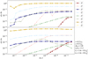 |
Fig. B.3 Values of the four integrals j1, j2, j4, j5 , both the real and imaginary part, as defined in Eq. (B.1) and Fig. B.2. The parameters used in the calculation are also presented in the figure. Each of the integrals is computed two times, for two values of |

We therefore conclude that the passage from Eq. (6) to Eq. (A.1) is justified by taking a large enough  and
and  , so that the error on the result is small compared to the result itself.
We now discuss the contribution to the integration given by the integrals j1 , j2, and j4. In Fig. B.3 we show the values of the four integrals j1 , j2 , j4 , I5 obtained numerically. This figure shows that the contribution of these integrals is small compared to j5 if  and
and  are sufficiently small.
We now discuss the validation of the numerical integration scheme presented in section A. The soundness of the numerical calculation of Eq. (A.1) is validated by multiple steps: considering the problem of integrating functions for which the analytical result is known, by validating the regularization strategy, and by considering physical limits in which the result is known. The steps of this procedure are detailed below.
First, a collection of functions for which the integral is known analytically Genz (1984) is used to test the numerical integration. The relative error between the numerical integration result and the value of the integral calculated analytically is presented in Fig. B.4, as a function of the parameter δabs..
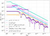 |
Fig. B.4 Convergence test for the numerical integration detailed in Appendix B, using the test functions from Genz (1984), with parameters a1 = a2 = 5 and ua = u2 = 0.5, in the integration region x, y ∊ [0, 1] × [0, 1]. |
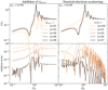 |
Fig. B.5 Mutual impedance spectrum, computed on the monopole emission and receiving geometry, for fpe / fce = 1.4. Different values for the δ parameter defined in Appendix A are presented (left), as well as different values of the normalized scattering frequencies fne / fpe defined in Eq. (4) (right). |
Second, the regularization strategy detailed in Sect. A for Eq. (A.1) is validated. This is done by comparing the results of the numerical calculation by either adding a small imaginary part to the denominator of Eq. (A.1) or using the collisional dielectric function Eq. (4). The results are presented in Fig. B.5. The two results are compatible in the case of δdenom. < 10−6 and fne / fpe < 10−4 . In this work, we chose to use the numerical regularization strategy of adding δdenom. = 10−8.
Third, the calculation of Eq. (A.1), is checked against previous results present in the literature (Gilet et al. 2017), in the unmagnetized limit of fce/ fpe → 0. In Fig. B.6 is presented the comparison between the two calculation, in the form of the mutual impedance spectrum for the RPC-MIP antenna presented in Fig. 6.
Fourth, at large distances from the emission antenna, compared to the Debye length, Eq. (6) tends to its value in the approximation of small temperatures (Kuehl 1974). A feature of the potential in this limit is the so-called interference cone structure (Kuehl 1973), present in two frequencies ranges: 0 < ω < min (ωpe , ωce) and max (ωpe , ωce) < ω < ωuh. This feature consists of a maximum of the potential at a specific angle θr.c. in physical space, and a series of secondary maxima for θ < θr.c. for 0 < ω < min (ωpe,ωce), and θ > θr.c. for max (ωpe, ωce) < ω < ωuh. In Fig. B.7 the amplitude and phase of the potential in Eq. (6) is presented at a fixed distance  as a function of the azimuthal angle. This is one example of the interference cone structure in the two frequency ranges, and is compatible with the results present in the literature (Kuehl 1973).
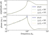 |
Fig. B.6 Mutual impedance spectrum expressed in Eq. (1) for the RPC- MIP configuration presented in Fig. 6. The amplitude (resp. the phase) is presented in the top (resp. bottom) panel. The Debye length is λDe = 10 cm. The continuous line is computed using the algorithm implemented in Gilet et al. (2017), while the dotted lines correspond to the calculation described in this work, for two values of the ratio fpe / fce of 10 and 50. |
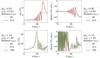 |
Fig. B.7 Electric potential amplitude (left) and phase (right) for f / fpe = 0.95 (resp. f/fpe = 1.14) and fpe/fce = 0.63 (resp. fpe/fec = 1.4) in the top (resp. bottom) figures. The continuous lines are consistent with the results of Kuehl (1973) Fig.2 (resp. Fig.7). |
The numerical approach to the calculation of Eq. (6) is thus considered validated.
Appendix C Examples of mutual impedance phase spectra in a magnetized plasma
In this appendix, we present the phase of the mutual impedance spectra presented in Sect. 4.1 and Sect. 4.2. They are shown in Fig. C.1 and Fig. C.2. To make these results more readable, we "unwrapped" the phase, meaning that adjacent values that have a difference larger than 180 degrees are substituted to their period-complementary values. In other words, if the phase goes from 360 degrees to 1 degrees, itis substituted with 361 degrees. From previous results in the unmagnetized limit, we expect to observe a change in the mutual impedance phase at a plasma resonance. A simplified discussion for the reason of this change is presented in Sect. 2. This behavior is observed also in the magnetized case at the upper-hybrid frequency, both in the case of a monopolar antenna Fig. C.1, and a quadrupolar antenna Fig. C.2. Changes in the phase are also visible at the fqn frequencies, even is they are less pronounced compared to the one at the upper-hybrid frequency. We also note that at frequencies much larger than the plasma frequency, the mutual impedance phase tends to zero. This is compatible with the intuition that at high frequency all the plasma modes become damped.
Appendix D Effect of geometry on mutual impedance experiments
In this appendix, we show the profound effects that the antenna geometry has on the expected mutual impedance spectrum. To do so, we consider the antenna geometry already used in Beghin (1995) and Gilet et al. (2017), with an emitting dipole and a receiving dipole. The dipole axes are perpendicular to one another. This geometry is a less symmetric version of the geometry compatible with the RPC-MIP experiment, considered in Sect. 4.2. In Fig. D.1 we present the results for this antenna geometry in the case of a varying magnetic field, to be compared with Fig. 5 and Fig. 6. In Fig. D.2 we present the results in the case of a varying electron-neutral scattering frequency, to be compared with Fig. 13. In Fig. D.3 we present the results in the case of a varying electron temperature anisotropy, to be compared with Fig. 9 and Fig. 10. In Fig. D.4 we present the results for the spectrum of the mutual impedance phase, to be compared with Fig. C.1 and Fig. C.2.
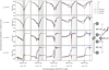 |
Fig. C.2 Phase of the mutual impedance spectrum for a quadrupolar antenna compatible with the one of the RPC-MIP instrument on board the Rosetta spacecraft, as presented in Fig. 6. |
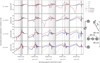 |
Fig. D.1 Mutual impedance spectrum for a quadrupolar configuration, according to the geometry presented in the figure, and also used by Beghin (1995) and Gilet et al. (2017). The parameters used for this calculation are the same used in Fig. 5. |
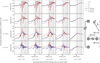 |
Fig. D.2 Mutual impedance spectrum for a quadrupolar configuration as the one used in Beghin (1995) and Gilet et al. (2017), with different values of the electron-neutral scattering frequencies presented in the horizontal axis, to be compared with Fig. 13. |
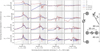 |
Fig. D.3 Mutual impedance spectrum for a quadrupolar antenna as the one used in Beghin (1995) and Gilet et al. (2017), with different electron temperature anisotropy, as in Fig. 9. |
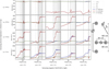 |
Fig. D.4 Phase of the mutual impedance spectrum for a quadrupolar antenna as the one in Beghin (1995) and Gilet et al. (2017), as presented in Fig. C.1 and Fig. C.2. |
References
- Alexandrov, A. F., Bogdankevich, L. S., & A., R. A. 1984, Principles of Plasma Electrodynamics (Springer) [Google Scholar]
- Andre, M. 1985, J. Plasma Phys., 33, 1 [Google Scholar]
- Bahnsen, A., Jespersen, M., Ungstrup, E., et al. 1988, Phys. Scr., 37, 469 [Google Scholar]
- Beghin, C. 1971, Space Research X1 (Berlin: Academic Verlag), SR X1, 1071 [Google Scholar]
- Beghin, C. 1995, Radio Sci., 30, 307 [NASA ADS] [CrossRef] [Google Scholar]
- Béghin, C., Berthelier, J. J., Debrie, R., et al. 1982, Adv. Space Res., 2, IN5 [Google Scholar]
- Béghin, C., Hamelin, M., Lebreton, J. P., et al. 2017, J. Geophys. Res. (Space Phys.), 122, 6964 [Google Scholar]
- Benkhoff, J., Murakami, G., Baumjohann, W., et al. 2021, Space Sci. Rev., 217, 90 [NASA ADS] [CrossRef] [Google Scholar]
- Bernhardt, P. A., Selcher, C. A., Lehmberg, R. H., et al. 2009, Ann. Geophys., 27, 4409 [Google Scholar]
- Bernstein, I. B. 1958, Phys. Rev., 109, 10 [NASA ADS] [CrossRef] [Google Scholar]
- Bhatnagar, P. L., Gross, E. P., & Krook, M. 1954, Phys. Rev., 94, 511 [Google Scholar]
- Bucciantini, L., Henri, P., Wattieaux, G., et al. 2022, J. Geophys. Res. (Space Phys.), 127, e2022JA030813 [Google Scholar]
- Bucciantini, L., Henri, P., Dazzi, P., et al. 2023a, J. Geophys. Res. (Space Phys.), 128, e2022JA031055 [Google Scholar]
- Bucciantini, L., Henri, P., Wattieaux, G., et al. 2023b, J. Geophys. Res. (Space Phys.), 128, e2023JA031534 [Google Scholar]
- Chasseriaux, J. M., R. Debrie, R. D., & C. Renard, C. R. 1972, J. Plasma Phys., 8, 231 [Google Scholar]
- Chisham, G., Schwartz, S. J., & Burgess, D. 1996, J. Geophys. Res., 101, 445 [Google Scholar]
- Christiansen, P., Gough, P., Martelli, G., et al. 1978, Nature, 272, 682 [Google Scholar]
- Décréau, P. M. E., Beghin, C., & Parrot, M. 1978, Space Sci. Rev., 22, 581 [Google Scholar]
- Décréau, P. M. E., Hamelin, M., Massif, R., de Feraudy, H., & Pawela, E. 1987, Ann. Geophys., 5, 181 [Google Scholar]
- Decreau-Prior, P. 1983, PhD thesis, Université d’Orléans E.E.R de sciences fondamentales et appliquées, France [Google Scholar]
- De Keyser, J., Ranvier, S., Maes, J., et al. 2021, in vEGU21, the 23rd EGU General Assembly, EGU21-7197 [Google Scholar]
- Demars, H. G., & Schunk, R. W. 1987, Rev. Geophys., 25, 1659 [Google Scholar]
- Derfler, H., & Simonen, T. C. 1969, Phys. Fluids, 12, 269 [Google Scholar]
- Dusenbery, P. B., & Kaufmann, R. L. 1980, J. Geophys. Res., 85, 5969 [Google Scholar]
- Fisher, R. K., & Gould, R. W. 1971, Phys. Fluids, 14, 857 [Google Scholar]
- Fischer, G., Panchenko, M., Macher, W., et al. 2021, Radio Sci., 56, e07309 [Google Scholar]
- Fried, B. D., & Conte, S. D. 1961, The Plasma Dispersion Function (Academic Press) [Google Scholar]
- Gary, S. P., & Cairns, I. H. 1999, J. Geophys. Res., 104, 19835 [Google Scholar]
- Gary, S. P., & Karimabadi, H. 2006, J. Geophys. Res. (Space Phys.), 111, A11224 [NASA ADS] [CrossRef] [Google Scholar]
- Gary, S. P., & Nishimura, K. 2003, Phys. Plasmas, 10, 3571 [NASA ADS] [CrossRef] [Google Scholar]
- Genz, A. 1984, in Proc. of International Conference on Tools, Methods and Languages for Scientific and Engineering Computation (USA: Elsevier North-Holland, Inc.), 81 [Google Scholar]
- Gilet, N. 2019, PhD thesis, Université d’Orléans, France [Google Scholar]
- Gilet, N., Henri, P., Wattieaux, G., Cilibrasi, M., & Béghin, C. 2017, Radio Sci., 52, 1432 [Google Scholar]
- Gilet, N., Henri, P., Wattieaux, G., et al. 2019, Front. Astron. Space Sci., 6, 16 [NASA ADS] [Google Scholar]
- Graham, D. B., Vaivads, A., Khotyaintsev, Y. V., et al. 2018, J. Geophys. Res. (Space Phys.), 123, 2630 [Google Scholar]
- Grard, R., Knott, K., & Pedersen, A. 1983, Space Sci. Rev., 34, 289 [Google Scholar]
- Grasset, O., Dougherty, M. K., Coustenis, A., et al. 2013, Planet. Space Sci., 78, 1 [Google Scholar]
- Haeusler, B., Haerendel, G., Bauer, O., et al. 1982, Sounding Rocket Program Magnetosphere. Project PORCUPINE, Final Report, Dec. 1979 Max-Planck-Inst. fuer Physik und Astrophysik, Garching (Germany, F.R.). Inst. fuer Extraterrestrische Physik [Google Scholar]
- Hamelin, M., Béghin, C., Grard, R., et al. 2007, Planet. Space Sci., 55, 1964 [NASA ADS] [Google Scholar]
- Kasaba, Y., Kojima, H., Moncuquet, M., et al. 2020, Space Sci. Rev., 216, 65 [NASA ADS] [CrossRef] [Google Scholar]
- Krall, N. A., & Trivelpiece, A. W. 1973, Principles of Plasma Physics (McGraw-Hill) [Google Scholar]
- Kuehl, H. H. 1973, Phys. Fluids, 16, 1311 [Google Scholar]
- Kuehl, H. H. 1974, Phys. Fluids, 17, 1275 [Google Scholar]
- Montgomery, M. D., Asbridge, J. R., & Bame, S. J. 1970, J. Geophys. Res., 75, 1217 [Google Scholar]
- Perraut, S., de Feraudy, H., Roux, A., et al. 1990, J. Geophys. Res., 95, 5997 [Google Scholar]
- Pfaff, R. F. 2012, Space Sci. Rev., 168, 23 [Google Scholar]
- Pottelette, R., Hamelin, M., Illiano, J. M., & Lembege, B. 1981, Phys. Fluids, 24, 1517 [Google Scholar]
- Roennmark, K. 1982, Waves in Homogeneous, Anisotropic Multicomponent Plasmas (WHAMP) [Google Scholar]
- Rohde, V., Piel, A., Thiemann, H., & Oyama, K. I. 1993, J. Geophys. Res., 98, 19163 [Google Scholar]
- Sarris, T. E., Talaat, E. R., Palmroth, M., et al. 2020, Geosci. Instrum. Methods Data Syst., 9, 153 [Google Scholar]
- Snodgrass, C., & Jones, G. H. 2019, Nat. Commun., 10, 5418 [NASA ADS] [CrossRef] [Google Scholar]
- Spencer, E., & Patra, S. 2015, Radio Sci., 50, 853 [Google Scholar]
- Stix, T. H. 1992, Waves in plasmas (Springer) [Google Scholar]
- Storey, L. R. O., Aubry, M. P., & Meyer, P. 1969, in Plasma Waves in Space and in the Laboratory, eds. J. O. Thomas, & B. J. Landmark (Edinburgh University Press), 303 [Google Scholar]
- Storey, L., Thiel, J., & Illiano, J. 1981, Project porcupine : the MF mutualimpedance probe experiment. Part I: Flight F2 (March 1977), Research report, Centre de recherches en physique de l’environnement terrestre et planétaire (CRPE) [Google Scholar]
- Štverák, Š., Trávníček, P., Maksimovic, M., et al. 2008, J. Geophys. Res. (Space Phys.), 113, A03103 [Google Scholar]
- Trotignon, J. G., Décréau, P. M. E., Rauch, J. L., et al. 2001, Ann. Geophys., 19, 1711 [Google Scholar]
- Trotignon, J. G., Michau, J. L., Lagoutte, D., et al. 2007, Space Sci. Rev., 128, 713 [NASA ADS] [CrossRef] [Google Scholar]
- Wattieaux, G., Gilet, N., Henri, P., Vallières, X., & Bucciantini, L. 2019, A&A, 630, A41 [NASA ADS] [CrossRef] [EDP Sciences] [Google Scholar]
- Wattieaux, G., Henri, P., Gilet, N., Vallières, X., & Deca, J. 2020, A&A, 638, A124 [NASA ADS] [CrossRef] [EDP Sciences] [Google Scholar]
- Yamauchi, M., De Keyser, J., Parks, G., et al. 2022, Exp. Astron., 54, 521 [NASA ADS] [Google Scholar]
All Figures
|
Fig. 1 Schematic drawing of the electric antenna configuration used in a typical quadrupolar mutual impedance experiment. The emitter antenna (E1-E2) is connected to the current generator, while the receiver antenna (R1-R2) is connected to the voltage measurement. |
| In the text | |
|
Fig. 2 Symmetric logarithmic representation of the real, panel a, and imaginary, panel b, part of the function |
| In the text | |
|
Fig. 3 Dispersion surfaces obtained with the numerical linearized Vlasov-Maxwell solver WHAMP, for a homogeneous, magnetized, and Maxwellian plasma (Roennmark 1982), for ne = 1.4 cm−3, Te = 2 eV, B = 132 nT, (fpe/fce = 2.88) presented all together (left) and separately, with color indicating the ratio of the magnetic to electric field (right) on a logarithmic scale. The frequency is normalized to electron plasma frequency, and the wave numbers, presented on a logarithmic scale, to the Debye length. |
| In the text | |
|
Fig. 4 In color, we present log10 |(fWHAMP − fe.s.)/fWHAMP|, where fWHAMP is the frequency obtained by the WHAMP (Roennmark 1982) solver in the general electromagnetic case, and fe.s. is the frequency obtained by solving the dispersion relation |
| In the text | |
|
Fig. 5 Mutual impedance spectrum for a monopolar antenna emission and reception, according to the geometry presented in the figure. The parameters used for this calculation are: from left to right, fpe/ fce = 5, 2, 1, 0.5, 0.2, and from bottom to top, λDe = 5, 10, 20, 40 cm. The different curves correspond to a different angle between the magnetic field and the emission-reception direction. |
| In the text | |
|
Fig. 6 Mutual impedance spectrum for a quadrupolar configuration, according to the geometry presented in the figure, and compatible with the one of the RPC-MIP instrument on board the Rosetta spacecraft. The parameters used for this calculation are the same used in Fig. 5. |
| In the text | |
|
Fig. 7 Hamelin’s diagram, which presents |
| In the text | |
|
Fig. 8 Analytical limits of different plasma instabilities generated by an electron temperature anisotropy; in particular, the electron mirror instability (Gary & Karimabadi 2006) (γ/ωce = 0.001), the whistler instability (Gary & Karimabadi 2006) (γ/ωce = 0.001), and the parallel and oblique fire-hose instability (Gary & Nishimura 2003) (γ/ωce = 0.01). |
| In the text | |
|
Fig. 9 Mutual impedance spectrum for a monopolar antenna configuration, as in Fig. 5, according to the geometry presented in the figure. Here, the ratio of plasma to electron cyclotron frequency is fpe/ fce = 1.4, as in Fig. 13. The electron temperature anisotropy, Te,⊥/Te,||, is presented on the horizontal axis increasing from left to right, and is considered in the model by the use of Eq. (5). |
| In the text | |
|
Fig. 10 Mutual impedance spectrum for a quadrupolar antenna compatible with the one of the RPC-MIP instrument, as in Fig. 6, with different electron temperature anisotropy, as in Fig. 9. |
| In the text | |
|
Fig. 11 Amplitude of the maxima at the first two fqn frequencies as a function of the angle between the magnetic field and the antenna emission-reception direction, for a monopolar geometry such as the one presented in Fig. 9. The amplitude increases as the angle approaches 90 degrees. |
| In the text | |
|
Fig. 12 Temporal damping rate, ℑ(f /fce), for the branch of Bernstein waves with 2 ⋅ fce ≤ f ≤ 3 ⋅ fce, presented as a function of the perpendicular (resp. parallel) wave number, k⊥ (resp. k||). The wave numbers are normalized relative to the parallel Larmor radius, rLe,|| = Tth,e,||/ωce, and fpe/fce = 1.4. Lines of a constant angle with the magnetic field are also presented. These results were obtained with the numerical linearized Vlasov-Maxwell solver WHAMP, for a homogeneous, magnetized, and Maxwellian plasma (Roennmark 1982). |
| In the text | |
|
Fig. 13 Mutual impedance spectrum for a quadrupolar configuration, according to the geometry presented in the figure, and compatible with the one of the RPC-MIP instrument on board the Rosetta spacecraft. Here, the ratio of plasma to electron cyclotron frequency is fpe/fce = 1.4. The effect of electron-neutral scattering, modeled by Eq. (4), is presented by the decreasing electron-neutral collision frequency on the horizontal axis, from left to right. |
| In the text | |
|
Fig. A.1 The progressively finer subdivisions produced by the numerical integration scheme is presented, using as an example one of the test functions from Genz (1984) that are used in the validation procedure described in appendix B. In the last figure, the function used in the integration is also shown in color. |
| In the text | |
|
Fig. B.1 Pseudocode form for the numerical integration algorithm used in this work to compute the values of the potential expressed by Eq. (A.1). |
| In the text | |
|
Fig. B.2 Illustration of the subdivision of the integration regions for the integral defined in Eq. (6), used in Eq. (B.1). |
| In the text | |
|
Fig. B.3 Values of the four integrals j1, j2, j4, j5 , both the real and imaginary part, as defined in Eq. (B.1) and Fig. B.2. The parameters used in the calculation are also presented in the figure. Each of the integrals is computed two times, for two values of |
| In the text | |
|
Fig. B.4 Convergence test for the numerical integration detailed in Appendix B, using the test functions from Genz (1984), with parameters a1 = a2 = 5 and ua = u2 = 0.5, in the integration region x, y ∊ [0, 1] × [0, 1]. |
| In the text | |
|
Fig. B.5 Mutual impedance spectrum, computed on the monopole emission and receiving geometry, for fpe / fce = 1.4. Different values for the δ parameter defined in Appendix A are presented (left), as well as different values of the normalized scattering frequencies fne / fpe defined in Eq. (4) (right). |
| In the text | |
|
Fig. B.6 Mutual impedance spectrum expressed in Eq. (1) for the RPC- MIP configuration presented in Fig. 6. The amplitude (resp. the phase) is presented in the top (resp. bottom) panel. The Debye length is λDe = 10 cm. The continuous line is computed using the algorithm implemented in Gilet et al. (2017), while the dotted lines correspond to the calculation described in this work, for two values of the ratio fpe / fce of 10 and 50. |
| In the text | |
|
Fig. B.7 Electric potential amplitude (left) and phase (right) for f / fpe = 0.95 (resp. f/fpe = 1.14) and fpe/fce = 0.63 (resp. fpe/fec = 1.4) in the top (resp. bottom) figures. The continuous lines are consistent with the results of Kuehl (1973) Fig.2 (resp. Fig.7). |
| In the text | |
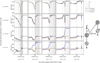 |
Fig. C.1 Phase of the mutual impedance spectrum for a monopolar antenna, as presented in Fig. 5. |
| In the text | |
|
Fig. C.2 Phase of the mutual impedance spectrum for a quadrupolar antenna compatible with the one of the RPC-MIP instrument on board the Rosetta spacecraft, as presented in Fig. 6. |
| In the text | |
|
Fig. D.1 Mutual impedance spectrum for a quadrupolar configuration, according to the geometry presented in the figure, and also used by Beghin (1995) and Gilet et al. (2017). The parameters used for this calculation are the same used in Fig. 5. |
| In the text | |
|
Fig. D.2 Mutual impedance spectrum for a quadrupolar configuration as the one used in Beghin (1995) and Gilet et al. (2017), with different values of the electron-neutral scattering frequencies presented in the horizontal axis, to be compared with Fig. 13. |
| In the text | |
|
Fig. D.3 Mutual impedance spectrum for a quadrupolar antenna as the one used in Beghin (1995) and Gilet et al. (2017), with different electron temperature anisotropy, as in Fig. 9. |
| In the text | |
|
Fig. D.4 Phase of the mutual impedance spectrum for a quadrupolar antenna as the one in Beghin (1995) and Gilet et al. (2017), as presented in Fig. C.1 and Fig. C.2. |
| In the text | |
Current usage metrics show cumulative count of Article Views (full-text article views including HTML views, PDF and ePub downloads, according to the available data) and Abstracts Views on Vision4Press platform.
Data correspond to usage on the plateform after 2015. The current usage metrics is available 48-96 hours after online publication and is updated daily on week days.
Initial download of the metrics may take a while.