| Issue |
A&A
Volume 697, May 2025
|
|
|---|---|---|
| Article Number | A202 | |
| Number of page(s) | 8 | |
| Section | Planets, planetary systems, and small bodies | |
| DOI | https://doi.org/10.1051/0004-6361/202450515 | |
| Published online | 23 May 2025 | |
Global asymmetric distributions of the low frequency whistler-mode waves in the Martian induced magnetosphere
1
Shandong Provincial Key Laboratory of Optical Astronomy and Solar-Terrestrial Environment, Institute of Space Sciences, Shandong University,
Weihai,
264209,
PR China
2
State Key Laboratory of Lunar and Planetary Sciences, Macau University of Science and Technology,
Macau,
PR China
★ Corresponding authors: This email address is being protected from spambots. You need JavaScript enabled to view it.
; This email address is being protected from spambots. You need JavaScript enabled to view it.
Received:
26
April
2024
Accepted:
5
March
2025
Abstract
Whistler-mode wave are vital electromagnetic waves that exist universally in the solar wind, shock, comet, and magnetosphere of magnetized celestial bodies. Recent studies have found that they can also be observed and locally generated in the induced magnetosphere of unmagnetized planets such as Mars. Whistler-mode wave distributions in the magnetosphere of magnetized celestial bodies are typically linked to the intrinsic dipole field morphology and solar wind-magnetosphere interaction. However, the global distribution pattern of these waves in the induced magnetosphere of Mars, an unmagnetized body, remains unclear. In this study, using observations from the Mars Atmosphere and Volatile Evolution (MAVEN) spacecraft, we for the first time find that the low frequency (f < 16 Hz) whistler-mode waves in the Martian induced magnetosphere show a hemisphere asymmetric distribution and B-minimum preference in the Mars-Solar-Electric (MSE) coordinate system. The wave occurrence rate is ∼ 1% in the vicinity of the center of the magnetotail in the –E hemisphere (ZMSE < 0) for XMSE < 0, and it is approximately ten times higher than that in the +E hemisphere (ZMSE > 0). Wave instability analyses based on the linear theory suggest that the global non-uniform background magnetic field and plasma density in the Martian induced magnetosphere caused by solar wind and Mars interactions can affect the wave growth rate, leading to a significant difference in wave occurrence between the ±E hemispheres. These wave properties are naturally distinct from the whistler-mode waves in the terrestrial magnetosphere with an intrinsic global dipole magnetic field. This study provides new insights for studying whistler-mode waves on unmagnetized celestial bodies with similar interactions between interstellar wind and ionosphere across the universe.
Key words: plasmas / waves / methods: statistical / solar wind / planets and satellites: terrestrial planets / planets and satellites: individual: Mars
© The Authors 2025
 Open Access article, published by EDP Sciences, under the terms of the Creative Commons Attribution License (https://creativecommons.org/licenses/by/4.0), which permits unrestricted use, distribution, and reproduction in any medium, provided the original work is properly cited.
This article is published in open access under the Subscribe to Open model. This email address is being protected from spambots. You need JavaScript enabled to view it. to support open access publication.
1 Introduction
Whistler-mode waves are naturally right-hand polarized transverse electromagnetic waves in space plasmas with a typical frequency of fLH < f < fce, where fLH and fce are the lower hybrid frequency and electron cyclotron frequency. The first report of whistler-mode waves was by the ground receiver, and it was generated by lightning (Helliwell 1967). The falling tone of the dispersive signals sounds similar to a whistle when converted into a sound signal, hence the name. Besides the Earth lightning whistler, whistler-mode waves have also been detected in solar wind, shocks, terrestrial space, planetary space, and comets (Horne & Thorne 2003; Li et al. 2010; Thorne et al. 2013; Meredith et al. 2013; Chen et al. 2014; Bai et al. 2023, 2024; Bai et al. 2023, Menietti et al. 2008; Harada et al. 2016; Tong et al. 2019; Tsurutani et al. 1989). The generation mechanism of whistler-mode waves is generally associated with various plasma instabilities caused by anisotropic particles through resonance (Kennel & Petschek 1966; Omura et al. 2008; Gurgiolo & D. 1993; Orlowski 1990; Hull et al. 2012). Once the resonant condition is satisfied, the waves and resonant electrons can exchange energy through interactions, leading to wave excitation or electron acceleration, diffusion, and precipitation (Horne & Thorne 2003; Thorne et al. 2010, 2013; Zong et al. 2008; Ni et al. 2011; Menietti et al. 2012; Su et al. 2014; Breneman et al. 2015; Artemyev et al. 2016; Zhang et al. 2022b).
In the terrestrial magnetosphere, the spatial distributions of whistler-mode waves have been extensively studied (Tsurutani & Smith 1974; LeDocq et al. 1998; Lauben et al. 2002; Santolík & Pickett 2004; Li et al. 2009), especially in the Van Allen Probes era (e.g., Cattell et al. 2015; Teng et al. 2018; Zhang et al. 2021; Shen et al. 2024). In situ observations suggest that whistler-mode waves show a latitude dependence and that the waves preferentially occur at the low latitude regions and dayside off-equatorial B-minimum regions (Tsurutani & Smith 1974; Santolík & Pickett 2004). The hot anisotropic electrons from the substorm injection mainly concentrate on the weak B regions due to the mirror effect, which contributes to wave generation (Li et al. 2010). The whistler-mode waves with B-minimum preference can also be found in some relatively small-scale magnetic field structures (Thorne & Tsurutani 1981; Kitamura et al. 2020; Zhang et al. 2019; Li et al. 2022; Tian et al. 2020; Ma et al. 2021). Whistler-mode waves can also be observed in the magnetosphere of unmagnetized planets such as Mars and Venus (e.g., Grard et al. 1989; Harada et al. 2016; Wang et al. 2023a,b; Ma et al. 2023a; Teng et al. 2023; Du et al. 2024; Russell et al. 2007). Although Mars may lack strong lightning due to its dilute atmosphere (Farrell et al. 2004) compared to Venus, solid evidence has been found that the crustal magnetic field in the southern hemisphere (see Figure 1a) can lead to a large electron anisotropy that is responsible for the local wave excitation via cyclotron resonance (Harada et al. 2016; Teng et al. 2023; Cheng et al. 2024). Recently, some case studies have reported instances of of whistler-mode waves inside the Martian induced magnetosphere far away from the region of the crustal magnetic field (Wang et al. 2023b; Ma et al. 2023a). Considering the potential influence of the whistler-mode waves on electron precipitation, heating, and ion escaping (Shane & Liemohn 2021), it is crucial to reveal and understand the global features of whistler-mode waves in the Martian induced magnetosphere.
The Martian induced magnetosphere is highly dynamic and variable since it is controlled by the upstream interplanetary magnetic field (IMF) and solar wind (Nagy et al. 2004; Carlsson et al. 2008; Wang et al. 2021; Liu et al. 2021; Dubinin et al. 2023). Previous studies suggest that the Martian induced magnetosphere exhibits some significant signatures if the coordinates are organized with respect to the upstream solar wind convection electric fields ESW (Dubinin et al. 2019). Such framing is referred to as Mars-Solar-Electric (MSE) coordinates, and when employed, the X axis points from Mars to the Sun, the Z axis is along ESW, and the Y axis completes the right-hand coordinate system and is approximately along the direction of upstream IMF (see Figure 1b). Some significant features of solar wind-Martian ionosphere interactions have been found in the MSE frame. The solar wind’s magnetic field can affect the magnetic field topology and modulate the behavior of charged particles. This includes ion plume escaping in the +E hemisphere, a closed magnetic field loop as well as a dense ion tail in the –E hemisphere, and the asymmetric (Dong et al. 2015; Dubinin et al. 2019; Chai et al. 2019; Harada et al. 2017; Zhang et al. 2022a; Ma et al. 2023b), resulting in complex magnetic topology around Mars. The distribution and regulation of whistler-mode waves in the Martian induced magnetosphere are still not fully understood, as both magnetic field and plasma density can influence the wave occurrence (Li et al. 2011; Ma et al. 2021). In this study, we use Mars Atmosphere and Volatile Evolution (MAVEN, Jakosky et al. 2015) observations to study the whistler-mode wave distributions in the Martian induced magnetosphere.
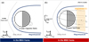 |
Fig. 1 Typical Martian magnetic field structures around Mars in the MSO (left) and MSE (right) coordinates. The term IMF refers to interplanetary magnetic field, ES W is solar wind convection electric field, and CS is current sheet. Typical crustal magnetic field structures in the southern hemisphere are only plotted in the MSO frame. |
2 Dataset and methods
We used the comprehensive MAVEN dataset from December 2014 to November 2019 to identify whistler-mode waves and determine the related parameters. The magnetometer (MAG; Connerney et al. 2015) provides 32 Hz magnetic field data, which is used to survey the whistler-mode signals. In this study, we only focus on whistler-mode waves with frequencies lower than 16 Hz , which is the maximum wave frequency identified using 32 Hz MAG data. We applied Fourier analyses to the magnetic field data using Means’s methods (Means 1972). We selected whistler signals statistically based on the wave properties using criteria similar to previous studies (Zhang et al. 2021): 1. the peak power of the magnetic field spectrogram should exceed 10−4 n T2 / Hz to ensure a large enough wave power rather than noise signals. 2. The power of the transverse component is larger than that of the compressional component. 3. The wave normal angle is smaller than 45±. 4. The ellipticity is larger than 0.7 to ensure right-hand polarization. 5. Polarization degree should be larger than 0.5. 6. The integrated wave amplitude above fL H should exceed 0.05 nT to exclude the noise from the four reaction wheel assemblies (Connerney et al. 2015). The duration for performing Fast Fourier transform is 2 seconds, and we defined the wave emission with a two-second time duration as a wave event. We note that the influence of the Doppler effect on the wave polarization can be ignored since the speed of the plasma flow in the Martian induced magnetosphere is typically low (several to tens of kilometers per second) (e.g., Dubinin et al. 2019).
To determine the plasma density, based on the quasi-neutral nature of plasma, we used the data from MAVEN’s Suprathermal and Thermal Ion Composition (STATIC; McFadden et al. 2015) instrument to calculate the total density of the main ion species 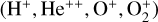 since the electron density from the Langmuir Probe and Waves (LPW, Andersson et al. 2015) measurements is not available for most of the orbiting times. Besides, determining electron density by moments calculation based on the electron 3D distribution data is inaccurate due to the large spacecraft potential, especially when MAVEN is in the Martian wake (Andreone et al. 2022).
We utilized one-second resolution MAG data and level 2 ion moments data of the Solar Wind Ion Analyzer (SWIA; Halekas et al. 2015) in the upstream solar wind as a proxy to establish the MSE coordinates when the whistler-mode waves are observed within the Martian induced magnetosphere. To obtain an accurate coordinate system, we only selected wave events with relatively stable solar wind conditions and whose angle variation between inbound and outbound IMF was less than 90± (e.g., Halekas et al. 2017; Chai et al. 2019). We also used magnetic field and ion moment data to identify the observations in the induced magnetosphere following the criteria outlined in Halekas et al. (2017).
According to the linear theory (Kennel & Petschek 1966), the growth rate γ of a whistler-mode wave is
![Mathematical equation: $\frac{\gamma }{\frame{\frame{f_\frame{ce}}}} = \pi \frame{\left(\nolbrace \frame{1 - \frac{f}{\frame{\frame{f_\frame{ce}}}}} \norbrace\right)^2}\eta \left(\nolbrace \frame{\frame{V_R}} \norbrace\right)\left[\nolbrace \frame{A\left(\nolbrace \frame{\frame{V_R}} \norbrace\right] - \frac{1}{\frame{\frame{f_\frame{ce}}/f - 1}}} \norbrace\right),$](/articles/aa/full_html/2025/05/aa50515-24/aa50515-24-eq2.png) (1)
where
(1)
where  represents the velocity of the resonant electrons; B, Ne, and me represent the background magnetic field intensity, electron density, and the electron mass, respectively; and η(VR) is the fraction of resonant electrons to the total electron population:
 (2)
(2)
Here, k is the wave number, F represents the electron distribution function, and v⊥ and v∥ the electron perpendicular and parallel velocity to the background magnetic field, respectively. The term A(VR) represents the anisotropy of the resonant electrons,
 (3)
the electron minimum cyclotron resonant energy is represented by
(3)
the electron minimum cyclotron resonant energy is represented by
 (4)
and the cyclotron resonance condition is
(4)
and the cyclotron resonance condition is
 (5)
where ω = 2 πf is the wave angular frequency, k∥ is the parallel wave number, and v∥ is the parallel speed of resonant electrons.
(5)
where ω = 2 πf is the wave angular frequency, k∥ is the parallel wave number, and v∥ is the parallel speed of resonant electrons.
We used the electron 3D burst mode data product provided by the MAVEN Solar Wind Electron Analyzer (SWEA; Mitchell et al. 2016) to calculate the wave growth rate. We first converted the original electron phase space density into the parameter space of v⊥ and v∥to form the distribution function F. For the whistler-mode waves with a specific wave frequency f, the minimum resonant energy ER is decided by formula (4). Finally, we used formulas (1)-(3) to get the wave growth rate for the corresponding resonant velocity VR.
3 Results
Figure 2 shows a typical case of whistler-mode waves observed in the Martian induced magnetosphere. During the time range from 08:15:00 UT to 08:21:00 UT on 10 February 2016, MAVEN orbited from [−1.2,−0.7,−0.2] to [−1.2,−0.7,−0.6] RM in MSO coordinates (in which case the X axis points from Mars to the Sun, the Y axis is along the anti-parallel direction of Mars’ orbital velocity, and the Z axis completes the right-hand coordinates). Figure 2c shows the total magnetic field intensity Bt and three components in MSO coordinates; Bt reached the local minimum at around 08:18:10 UT. The relatively weak Bt is accompanied by large ion populations (Figure 2e). Figures 22h–k display the frequency spectrograms of the transverse and compressional magnetic field components, the wave normal angle, and the ellipticity of the 32 Hz magnetic field data analyzed using Mean’s method (Means 1972). At ∼ 08: 18 UT, clear wave signals with a frequency higher than the local lower hybrid frequency were detected by MAVEN. The dominant component is transverse, and the right-hand polarized signals with a wave normal angle less than 45± (Figure 2j) and an ellipticity larger than 0.7 indicate that the wave signals are whistler-mode waves. The observed whistler-mode waves in Figure 2 have a broad frequency ranging from ∼ 5 to ∼ 13 Hz, with a central frequency of ∼ 0.07 fc e, while the electron cyclotron frequency fc e is ∼ 101 Hz. We then calculated the minimum resonant energy for the ∼ 0.07 fc e whistler-mode waves as indicated by the black line in the electron energy spectrogram (Figure 2f). A significant decrease of the electron resonant energy was found around 08:18 UT due to the weak Bt and larger plasma density. The electrons with resonant energy ranging from ∼ 20 to ∼ 50 eV exhibit perpendicular anisotropy as indicated by the electron pitch angle distribution (Figure 2g), which indicates that these anisotropic electrons could generate the observed ∼ 5 to ∼ 13 Hz whistlermode waves via cyclotron resonance. This is also supported by the linear instability analyses shown in Figure 1j, where the wave growth rate γ reaches a high value (∼ 0.01 fc e−1) in the large wave amplitude region.
Using the dataset and criteria described in Section 2, we identified a total of 75655 whistler-mode wave events, with each covering a time interval of 2 seconds. To highlight the key spatial distribution characteristics of magnetospheric whistlermode waves, the distributions of MAVEN’s orbit density, the number of wave events, and the wave occurrence rate in two cross-sectional planes of the magnetosphere, the XZ plane (Figures 3a–3c) and the YZ plane (Figures 3d–3f) in the MSE coordinates are displayed in Figure 3. The data in the XZ plane are constrained to |YM S E|<0.5 RM, while those in the YZ plane are limited to XM S E<0. The size of each bin is 0.125 RM × 0.125 RM. The wave occurrence rate is calculated by dividing the whistler-mode wave signal numbers by the orbit density in each XZ or YZ bin. The bins with insufficient sampling duration (less than 0.5 hours in the XY plane and less than 1 hour in the YZ plane) are ignored to maintain statistical validity. A significant asymmetry can be seen in Figures 3c and 3f, where the wave occurrence rate is approximately ten times higher in the +E hemisphere (∼ 1 %) than in the +E hemisphere (∼ 0.1 %) near the center of the magnetotail for XM S E<0. The occurrence rate of the whistler-mode waves is also high near the magnetic pile-up boundary on the dayside (XM S E>0) induced magnetosphere. This could be attributed to the penetration of waves originating from the magnetosheath (e.g., Harada et al. 2016). In the following analyses, we only focus on the whistler-mode waves far from the dayside magnetic pile-up boundary since the propagation effect from the magnetosheath is beyond the scope of this study. Therefore, the whistler-mode waves at XM S E<0 are of particular interest in this study.
To examine the distribution of whistler-mode waves and their relation to the magnetic topology of the induced magnetosphere, we organized the whistler-mode wave occurrence and some key parameters into B xM S E −ZM S E space (Figure 4). Figure 4a shows the normalized density distribution of wave events in the B xM S E −YM S E space. The normalization divides the data numbers in each B xM S E −YM S E bin by the total number of data points at the particular B xM S E bin. The positive (negative) Bx is mainly distributed in negative (positive) YM S E regions, indicating that the center of the Martian magnetic tail current sheet is located near YM S E = 0. The wave occurrence is highest in the center of the Martian magnetotail (−5 nT<B xM S E>5 nT) and well constrained by the weak Bt regions, as indicated by the white contour lines of 0.4 % wave occurrence rate in Figures 4b and 4c. The median wave frequency is ∼ 0.035 fc e (Figure 4 g). Therefore, we used the linear theory to calculate γ(VR), η(VR), A(VR), and E(VR) of whistler-mode waves (see Equations (1)–(4)) at a frequency of f = 0.035 fc e. Considering the finite field of view of SWEA, we excluded the data with a blocked pitch angle larger than 30± (e.g., Harada et al. 2016) to ensure the validity of the calculation. In Figure 4d, the large γ(VR) is well constrained by the white contour curve representing a 0.4 % wave occurrence rate in B xM S E −ZM S E space. Only positive γ(VR) is considered here since the negative γ(VR) does not contribute to the wave growth. The median value of positive γ(VR) is generally ∼ 10−3 fc e inside the contour line, which is several factors of ten higher than ∼ 10−5−10−4 fc e outside, indicating a potential increase in wave growth in the weak Bt regions. Both γ(VR) and η(VR) exhibit a significant asymmetry in which the median value in the −E hemisphere is approximately ten times higher than that in the +E hemisphere for the B xM S E range of [−5,5] nT. However, the anisotropy of the resonant electrons A(VR) does not show such an asymmetry (Figure 4f). This indicates that the major contribution to γ(VR) is η(VR) compared to A(VR) since η(VR) shows a similar distribution with γ(VR) in B xM S E −ZM S E space. Asymmetric signatures can be seen in the distributions of Bt and N with ZM S E (Figures 4c and 4h). The weak Bt(∼ 4 nT) and large plasma density (∼ 10 cm−3) result in a lower E(VR) of 10 s eV in the −E hemisphere, which is approximately ten times lower than that in the + E hemisphere (Figure 4i). This E(VR) trough in the −E hemisphere can account for the larger η(VR) since a lower resonant energy generally corresponds to a larger resonant electron population (see Figure 2f) and therefore a statistically larger γ(VR). The above observational and theoretical results indicate that the distinctive magnetic field and plasma structures of the Martian induced magnetosphere can regulate the asymmetric distributions of whistler-mode waves between hemispheres.
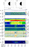 |
Fig. 2 Overview of a whistler-mode wave case. (a) Wave location (blue triangle) in the MSE-XY plane. (b) Wave location (blue triangle) in the XZ plane. (c) Total magnetic field intensity Bt (black) and three components (blue: Bx, green: By, and red: Bz) in MSO coordinates. (d) Ion mass spectrogram. (e) Plasma density. (f) Electron energy spectrogram with the minimum cyclotron resonant energy of 0.07 fc e whistler-mode waves (black line). (g) Pitch angle distributions of the electrons with energy ̌20 eV. Frequency spectrograms of (h) transverse and (i) parallel components of the magnetic field. (j) Wave normal angle and (k) ellipticity. (1) Integrated wave amplitude with frequency higher than the lower hybrid frequency fL H. (m) Theoretical linear wave growth rate. The dashed and solid curves in (a) and (b) represent the nominal location of the Martian magnetic pile-up boundary and bow shock (Trotignon et al. 2006). White lines in (h, i, m) and black lines in (j, k) represent fL H. |
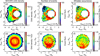 |
Fig. 3 Spatial distributions of the (a and d) MAVEN orbit density, (b and e) whistler-mode wave signal numbers, and (c and f) wave occurrence rate on the XZ (−0.5 RM < YM S E < 0.5 RM) and YZ (XM S E < 0) planes in MSE coordinates. Bins with an insufficient sampling rate (orbit density less than 0.5 hours for the XZ plane and 1 hour for the YZ plane) are ignored in (b), (c), (e), and (f). Curves in (a-c) represent the nominal location of the Martian magnetic pile-up boundary (Trotignon et al. 2006). |
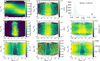 |
Fig. 4 Distributions of (a) the normalized data density in B xM S E − YM S E space. (b) Whistler-mode wave occurrence, medians of (c) total magnetic field intensity Bt, (d) the positive linear waves growth rate γ(VR) / fc e, (e) η(VR), (f) A(VR), (h) plasma density, and (i) E(VR) in the B xM S E − ZM S E space. Panel (g) represents normalized frequency distributions of whistler-mode waves. Data bins with sampling of less than 10 minutes in (d)-(i) are colored gray. The terms γ(VR), η(VR), E(VR), and A(VR) were calculated with wave frequency f = 0.035 fc e. The overlapped white curves in (b) and (d)-(i) are the contour line of the 0.4% occurrence rate of whistler-mode waves. |
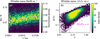 |
Fig. 5 (a) Distributions of the normalized density of the normalized wave amplitude Bw / B and the corresponding linear normalized wave growth rate γ / fc e. White dots represent the median Bw / B in γ bins, and the magenta line represents the fitting line of these white dots. (b) Distributions of whistler wave signals in the (Δ f /⟨ f⟩, σ) parameter space. The magenta line represents Δ f /⟨ f⟩=σ. |
4 Discussion
4.1 Regime of the wave-particle interaction
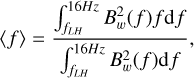
Previous studies have found that the normalized amplitude of saturated whistler-mode waves (Bw / B) is proportional to the linear wave growth rate: Bw / B = Q (γ / fc e)κ (Tao et al. 2017; Kuzichev et al. 2019). Figure 5 shows the normalized density of observed whistler-mode waves in the (Bw / B, γ / fc e) parameter space. The normalization divides the number of events in each Bw / B−γ / fc e bin by the total number of wave events at the particular γ / fc e bin. One can notice that the normalized wave amplitude Bw / B of whistler-mode waves generally increases with the intensity of the linear wave growth rate. The white dots in Figure 5 denote the median value of Bw / B for each γ / fc e bin. The fitting function of these white dots is Bw / B = 0.05(γ / fc e)0.15, with parameters Q = 0.05 and κ = 0.15. The monotonically increasing trend of Bw / B with γ / fc e suggests an efficient wave growth by the anisotropic electrons. We emphasize here that κ may be underestimated due to the scatter effect of whistler-mode waves on the electron distribution function (e.g., Gao et al. 2022) or non-local origin. However, evaluating the wave propagating effect is difficult since the Poynting flux of waves is not available due to the data limitation. Moreover, to determine the regime of waveparticle interaction, we evaluated the wave bandwidth Δ f /⟨ f⟩ and the wave intensity parameter 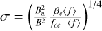 (Shapiro & Sagdeev 1997; Karpman 1974), where βe = 8 π Ne Te / B2 and Te represents the electron temperature. The averages of the wave frequency ⟨ f ⟩, frequency bandwidth Δ f, and Bw of whistlermode waves are derived from the power spectral density of the magnetic field Bw2(f) using the following equations:
 (6)
(6)
 (7)
(7)
 (8)
(8)
The validity of the linear hypothesis depends on the relationship between Δ f /⟨ f⟩ and σ (Shapiro & Sagdeev 1997). For the whistler-mode waves with (Δ f /⟨ f⟩ ≫ σ), the wave spectrum width is broad, and the regime of wave-particle interaction is linear. Conversely, when (Δ f /⟨ f⟩ ≪ σ), the wave intensity is high enough to sustain nonlinear wave-particle interactions (Karpman 1974). As shown in Figure 5c, more than 99 % of the whistler-wave signals in our work are located above the magenta line (Δ f /⟨ f⟩ = σ), indicating that the linear wave-particle interaction is the main process, which verifies the applicability of the linear analyses in our study. This differs from the narrow band whistler-mode waves with a rising tone in the Martian crustal magnetic field, where non-linear processes due to the non-uniform background magnetic field have been demonstrated (Teng et al. 2023). One should note that the limitation of the frequency band will cause some inaccuracy due to the underestimated Δ f and Bw when the peak frequency of the whistler-mode wave is high. However, this effect may not be significant, as the peak frequency of most whistler-mode waves is low (<6 Hz).
4.2 Electron pitch angle distributions
We also investigated which distinct shapes of the electron distribution can lead to the observed waves. Figure 6 shows the electron pitch angle distributions for two energy ranges (E< 30 eV and E>30 eV) in the whistler-mode wave events. The ionospheric photoelectrons typically have a peak flux between 22 and 27 eV (e.g., Xu et al. 2019). We chose 30 eV as a rough threshold to distinguish between ionospheric cold electrons (<30 eV) and those originating from the solar wind. Statistically, the lower energy electrons (E< 30 eV) exhibit small anisotropy. In contrast, the E>30 eV electrons show perpendicular anisotropy, with a higher perpendicular flux than the parallel and anti-parallel fluxes (Figures 6a and 6d). This perpendicular anisotropy for E>30 eV electrons is associated with cyclotron resonance and contributes to wave excitation. We further separated the dataset into two groups, waves with radially outward (Br>0) and inward (Br < 0) magnetic fields, in order to examine the magnetic topology. Figures 6e and 6f show that the parallel (anti-parallel) flux of hot electrons is slightly reduced for positive (negative) Br. One possible explanation for this is that the magnetic topology in part of the wave events is open field lines with one side connected to the ionosphere, as indicated by the lower flux of outward hot electrons than the inward hot electrons (e.g., Xu et al. 2019). Moreover, electron perpendicular anisotropy can be caused by a closed field line configuration (e.g., Harada et al. 2016), magnetic reconnection (e.g., Wang et al. 2023b), the mirror effects resulting from the local B-minimum (e.g., Ma et al. 2023a), and the betatron acceleration in the magnetic peak (e.g., Fu et al. 2011). Considering the complexity of the magnetic topology around Mars, exploring the dependence of electron anisotropy on the magnetic topology would be intriguing, and we leave it to a future study.
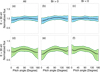 |
Fig. 6 Statistical electron pitch angle distributions for different energy ranges in whistler-mode waves. The top and bottom rows are for E< 30 eV and E>30 eV, while the left, middle, and right columns are for all Br>0 and Br<0 wave events. The black lines and the upper and lower boundaries of blue or green shaded regions represent the median value, upper, and lower quartiles of the normalized flux as a function of electron pitch angle. |
4.3 Comparison with the other celestial bodies
In celestial bodies with a dense atmosphere or intrinsic magnetic fields, the generation of whistler-mode waves is associated with lightning activity, unstable plasmas, and plasma density structures (e.g., Helliwell 1967; Russell et al. 2007; Li et al. 2010; Bortnik et al. 2008; Meredith et al. 2013; Chen et al. 2014; Mauk et al. 1997; George et al. 2023; Ozaki et al. 2023). Highly anisotropic energetic (> 10 ke V) electrons during storm time are considered the main source of whistler-mode chorus waves in the terrestrial magnetosphere (Li et al. 2010), which further form the plasmaspheric whistler-mode hiss waves (Bortnik et al. 2008). In other words, the A(VR) plays an important role in controlling wave generation in the terrestrial magnetosphere. For the whistler-mode waves with a typical frequency of ∼ 0.035 fc e in the Martian induced magnetosphere, the median A(VR) is generally higher than the critical anisotropy Ac(VR) = 1 /(fc e / f−1) (∼ 0.036) in the weak B regions, while A(VR) does not exhibit a significant hemispheric asymmetry in the MSE frame (see Figure 4f). Therefore, the global modulation of wave growth rate in the Martian induced magnetosphere depends more on η(VR) rather than A(VR), which is different from the waves in the terrestrial magnetosphere. We also point out that this discussion is only for the low frequency whistler-mode waves. It would be intriguing to compare the modulation characteristics of the higher frequency (> 16 Hz) whistler-mode waves measured with higher resolution instruments by future missions to our results.
We note that most (∼ 84 %) of our whistler-mode wave events have an electron temperature anisotropy Te ⊥ / Te | larger than one, indicating the generation mechanism of cyclotron resonance. Thus, we argue that the whistler-mode waves in our study are intrinsically different in their generation mechanisms compared to the low frequency whistler-mode waves excited by electron beam distribution (Gary & Feldman 1977; Huang et al. 2016; An et al. 2017; Wang et al. 2022) or the relative drift between ions and electrons (Hellinger & Mangeney 1997; Balikhin et al. 1997; Wilson et al. 2012; Hull et al. 2020; Wang et al. 2024). The latter typically have a large wave amplitude (Bw / B ∼ 1) and are frequently observed upstream of the bow shock of various celestial bodies (e.g., Wilson et al. 2012; Brain et al. 2002; Ruhunusiri et al. 2018; Xiao et al. 2020; Lou et al. 2023). In addition, the absence of the counter-streaming core and halo electrons from the solar wind in our wave events does not support the mechanism of heat flux instability that the quasi-linear propagating whistler-mode waves can also be generated from (Gary et al. 1975; Lacombe et al. 2014; Stansby et al. 2016; Tong et al. 2019). The highly correlated spatial distribution between wave occurrence and wave growth rate along with the small wave amplitude (Bw / B ∼ 0.01) and wave-particle interaction regime analyses (see Figure 5) support the mechanism of linear instability caused by anisotropic electrons in our events.
We further discuss the formation of the B minimum pocket effect in the Martian induced magnetosphere’s −E hemisphere. The Martian induced magnetosphere shows various hemispheric asymmetric features in the MSE coordinates (Dubinin et al. 2017, 2019; Chai et al. 2019). Other unmagnetized bodies such as Venus and Titan exhibit similar characteristics in their induced magnetosphere (Dubinin et al. 2013; Chai et al. 2016; Bertucci et al. 2008). In the interaction process between solar wind and the Martian ionosphere, the extra momentum carried by the pick-up ions from the ionosphere affect the field line topology draped around Mars in the direction of ES W (Dubinin et al. 2019). As these field lines wrap around Mars in the E hemisphere, the magnetic loop and the weak magnetic field intensity regions are therefore formed. This further prevents planetary ions from escaping tailward and produces a dense ion tail in the −E hemisphere (Dubinin et al. 2019), as shown in Figure 4h. The B-minimum and dense plasma density tail in the - E hemisphere therefore provide a suitable environment for the resonance trough for wave generation. This new distribution pattern is naturally distinct from the whistler-mode waves in the magnetospheres of Earth, Jupiter, and Saturn, the magnetized bodies where the wave occurrence preference depends on their intrinsic global dipole magnetic field and the structures resulting from the solar wind-magnetosphere interactions (Tsurutani & Smith 1974; Santolík & Pickett 2004; Teng et al. 2018; Menietti et al. 2008; Li et al. 2020; Ozaki et al. 2023).
5 Conclusion
In conclusion, using MAVEN in situ measurements, we have discovered a hemispheric asymmetric pattern of the low frequency whistler-mode wave distributions in the Martian induced magnetosphere for the first time. The wave occurrence rate is ∼ 1 % in the −E hemisphere (ZM S E < 0) for XM S E < 0, about an order higher than that in the + E hemisphere (ZMSE > 0) of the MSE coordinates. Our analyses suggest that weaker Bt and higher electron densities in the −E hemisphere, caused by the convective electric field, decrease the cyclotron resonant energy. Together with the higher fraction of resonant particles (the consequence of the weaker Bt and higher electron densities), this results in a higher growth rate of the whistler-mode waves than in the +E hemisphere. This is different from the case in the terrestrial magnetosphere in which the whistler-mode wave occurrence is highly dependent on the energetic anisotropic electrons from the magnetospheric substorm process due to the interactions between the solar wind and the intrinsic dipole magnetic field. We speculate that this new pattern of whistler-mode wave distributions in the Martian induced magnetosphere can generally exist in various unmagnetized bodies due to their similar interactions between the stellar wind and ionosphere. Again, we acknowledge that the wave survey in this study has some limitations due to the finite time resolution of the MAG data. Only low frequency (f<16 Hz) whistler-mode waves can be collected under this dilemma. Future Mars space missions equipped with higher-resolution magnetic and electric field instruments will provide a better wave survey and a deeper understanding of the whistler-mode waves.
Acknowledgements
We thank the entire MAVEN team for the usage of the data. MAVEN data are publicly available through the Planetary Data System (https://pds-ppi.igpp.ucla.edu/mission/MAVEN). The authors would like to thank Dr. M. M. Wang for the helpful suggestions. This work is supported by the National Natural Science Foundation of China (Grants 42275135, 423B2410, 42104153, and 42274220), the Natural Science Foundation of Shandong Province (Grants ZR2022QD135, ZR2023JQ016, and ZR2024MD050), and the Science and Technology Development Fund, Macau SAR (File No. SKL-LPS(MUST)-2021-2023).
References
- An, X., Bortnik, J., Van Compernolle, B., Decyk, V., & Thorne, R. 2017, Phpl, 924, L34 [Google Scholar]
- Andersson, L., Ergun, R. E., Delory, G. T., et al. 2015, SSRv, 195, 173 [Google Scholar]
- Andreone, G., Halekas, J. S., Mitchell, D. L., Mazelle, C., & Gruesbeck, J. 2022, JGR, 127, e2021JA029404 [Google Scholar]
- Artemyev, A., Agapitov, O., Mourenas, D., et al. 2016, SSRv, 200, 261 [Google Scholar]
- Bai, S., Shi, Q., Zhang, H., et al. 2023, JGR, 128, e2023JA031816 [Google Scholar]
- Bai, S., Shi, Q., Shen, X., et al. 2024, JGR, 129, e2024JA032986 [Google Scholar]
- Balikhin, M. A., Walker, S. N., Dudok de Wit, T., et al. 1997, AdSR, 20, 729 [Google Scholar]
- Bertucci, C., Achilleos, N., Dougherty, M. K., et al. 2008, Science, 321, 1475 [Google Scholar]
- Bortnik, J., Thorne, R. M., & Meredith, N. P. 2008, Nature, 452, 62 [Google Scholar]
- Brain, D. A., Bagenal, F., Acuña, M. H., et al. 2002, JGR, 107, 1076 [Google Scholar]
- Breneman, A. W., Halford, A., Millan, R., et al. 2015, Nature, 523, 193 [Google Scholar]
- Carlsson, E., Brain, D., Luhmann, J., et al. 2008, P&SS, 56, 861 [Google Scholar]
- Cattell, C. A., Breneman, A. W., Thaller, S. A., Wygant, J. R., & Kletzing, C. A. 2015, GeoRL, 42, 7273 [Google Scholar]
- Chai, L., Wei, Y., Wan, W., et al. 2016, JGR, 121, 688 [Google Scholar]
- Chai, L., Wan, W., Wei, Y., et al. 2019, ApJ, 871, L27 [Google Scholar]
- Chen, L., Thorne, R. M., Bortnik, J., et al. 2014, GeoRL, 41, 5702 [Google Scholar]
- Cheng, S., Su, Z., Wu, Z., & Wang, Y. 2024, GeoRL, 51, e2023GL106695 [Google Scholar]
- Connerney, J. E. P., Espley, J., Lawton, P., et al. 2015, SSRv, 195, 257 [Google Scholar]
- Dong, Y., Fang, X., Brain, D. A., et al. 2015, GeoRL, 42, 8942 [Google Scholar]
- Du, H., Cao, X., Ni, B., et al. 2024, JGR, 129, e2023JA032210 [Google Scholar]
- Dubinin, E., Fraenz, M., Zhang, T. L., et al. 2013, JGR, 118, 7624 [Google Scholar]
- Dubinin, E., Fraenz, M., Pätzold, M., et al. 2017, JGR, 122, 4009 [Google Scholar]
- Dubinin, E., Modolo, R., Fraenz, M., et al. 2019, GeoRL, 46, 12722 [Google Scholar]
- Dubinin, E., Fraenz, M., Pätzold, M., et al. 2023, JGR, 128, e2022JA030575 [Google Scholar]
- Farrell, W. M., Smith, P. H., Delory, G. T., et al. 2004, JGR, 109, E03004 [Google Scholar]
- Fu, H. S., Khotyaintsev, Y. V., André, M., & Vaivads, A. 2011, GeoRL, 38, 16 [Google Scholar]
- Gao, L., Vainchtein, D., Artemyev, A. V., & Zhang, X. 2022, JGR, 127, e30603 [Google Scholar]
- Gary, S. P., & Feldman, W. C. 1977, JGR, 82, 1087 [Google Scholar]
- Gary, S. P., Feldman, W. C., Forslund, D. W., & Montgomery, M. D. 1975, JGR, 80, 4197 [Google Scholar]
- George, H., Malaspina, D. M., Goodrich, K., et al. 2023, GeoRL, 50, 19 [Google Scholar]
- Grard, R., Pedersen, A., Klimovt, S., et al. 1989, Nature, 341, 607 [NASA ADS] [CrossRef] [Google Scholar]
- Gurgiolo, C., W. H. K., & D., W. 1993, GeoRL, 20, 783 [Google Scholar]
- Halekas, J. S., Taylor, E. R., Dalton, G., et al. 2015, SSRv, 195, 125 [Google Scholar]
- Halekas, J. S., Ruhunusiri, S., Harada, Y., et al. 2017, JGR, 122, 547 [Google Scholar]
- Harada, Y., Andersson, L., Fowler, C. M., et al. 2016, JGR, 121, 9717 [Google Scholar]
- Harada, Y., Halekas, J. S., McFadden, J. P., et al. 2017, JGR, 122, 5114 [Google Scholar]
- Hellinger, P., & Mangeney, A. 1997, JGR, 102, 9809 [Google Scholar]
- Helliwell, R. A. 1967, JGR, 72, 4773 [Google Scholar]
- Horne, R. B., & Thorne, R. M. 2003, GeoRL, 30, 1527 [Google Scholar]
- Huang, S. Y., Fu, H. S., Yuan, Z. G., et al. 2016, JGR, 121, 6639 [Google Scholar]
- Hull, A. J., Muschietti, L., Oka, M., et al. 2012, JGR, 117, A12104 [Google Scholar]
- Hull, A. J., Muschietti, L., Le Contel, O., Dorelli, J. C., & Lindqvist, P. 2020, JGR, 125, 7 [Google Scholar]
- Jakosky, B. M., Lin, R. P., Grebowsky, J. M., et al. 2015, SSRv, 195, 3 [Google Scholar]
- Karpman, V. I. 1974, SSRv, 16, 361 [Google Scholar]
- Kennel, C. F., & Petschek, H. E. 1966, JGR, 71, 1 [NASA ADS] [CrossRef] [Google Scholar]
- Kitamura, N., Omura, Y., Nakamura, S., et al. 2020, JGR, 125, e2019JA027488 [Google Scholar]
- Kuzichev, I. V., Vasko, I. Y., Soto-Chavez, A. R., et al. 2019, ApJ, 882, 81 [Google Scholar]
- Lacombe, C., Alexandrova, O., Matteini, L., et al. 2014, ApJ, 796, 1 [NASA ADS] [CrossRef] [Google Scholar]
- Lauben, D. S., Inan, U. S., Bell, T. F., & Gurnett, D. A. 2002, JGR, 107, 1429 [Google Scholar]
- LeDocq, M. J., Gurnett, D. A., & Hospodarsky, G. B. 1998, GeoRL, 25, 4063 [Google Scholar]
- Li, W., Thorne, R. M., Angelopoulos, V., et al. 2009, JGR, 114, A00C14 [Google Scholar]
- Li, W., Thorne, R. M., Nishimura, Y., et al. 2010, JGR, 115, A06205 [Google Scholar]
- Li, W., Thorne, R. M., Bortnik, J., Nishimura, Y., & Angelopoulos, V. 2011, JGR, 116, A00F11 [Google Scholar]
- Li, W., Shen, X.-C., Menietti, J. D., et al. 2020, GeoRL, 47, e88198 [Google Scholar]
- Li, L., Omura, Y., Zhou, X., et al. 2022, GeoRL, 49, 10 [Google Scholar]
- Liu, D., Rong, Z., Gao, J., et al. 2021, ApJ, 911, 113 [NASA ADS] [CrossRef] [Google Scholar]
- Lou, Y., Gu, X., Cao, X., et al. 2023, ApJ, 943, 2 [Google Scholar]
- Ma, X., Tian, A. M., Shi, Q. Q., et al. 2021, GeoRL, 48, e2021GL095730 [Google Scholar]
- Ma, X., Tian, A., Bai, S., et al. 2023a, ApJ, 956, 5 [Google Scholar]
- Ma, X., Tian, A., Guo, R., et al. 2023b, Icarus, 406, 115758 [Google Scholar]
- Mauk, B. H., Williams, D. J., & McEntire, R. W. 1997, GeoRL, 24, 2949 [Google Scholar]
- McFadden, J. P., Kortmann, O., Curtis, D., et al. 2015, SSRv, 195, 199 [Google Scholar]
- Means, J. D. 1972, JGR, 77, 5551 [Google Scholar]
- Menietti, J. D., Horne, R. B., Gurnett, D. A., et al. 2008, AnGeo, 26, 1819 [Google Scholar]
- Menietti, J. D., Shprits, Y. Y., Horne, R. B., et al. 2012, JGR, 117, A12214 [Google Scholar]
- Meredith, N. P., Horne, R. B., Bortnik, J., et al. 2013, GeoRL, 40, 2891 [Google Scholar]
- Mitchell, D. L., Mazelle, C., Sauvaud, J. A., et al. 2016, SSRv, 200, 495 [Google Scholar]
- Nagy, A. F., Winterhalter, D., Sauer, K., et al. 2004, SSRv, 111, 33 [Google Scholar]
- Ni, B., Thorne, R. M., Meredith, N. P., Horne, R. B., & Shprits, Y. Y. 2011, JGR, 116, A04219 [Google Scholar]
- Omura, Y., Katoh, Y., & Summers, D. 2008, JGR, 113, A4 [Google Scholar]
- Orlowski, D. S., Crawford, G. K., & Russell, C. T. 1990, GeoRL, 17, 2293 [Google Scholar]
- Ozaki, M., Yagitani, S., Kasaba, Y., et al. 2023, Nat. Astron., 7, 1309 [Google Scholar]
- Ruhunusiri, S., Halekas, J. S., Espley, J. R., et al. 2018, JGR, 123, 3460 [Google Scholar]
- Russell, C. T., Zhang, T. L., Delva, M., et al. 2007, Nature, 450, 661 [CrossRef] [Google Scholar]
- Santolík, O. D. G., & Pickett, J. 2004, AnGeo, 22, 2555 [Google Scholar]
- Shane, A., & Liemohn, M. 2021, JGR, 126, e2021JA029118 [Google Scholar]
- Shapiro, V. D., & Sagdeev, R. Z. 1997, PhyR, 283, 49 [Google Scholar]
- Shen, X., Li, W., Ma, Q., et al. 2024, GeoRL, 51, e2023GL106681 [Google Scholar]
- Stansby, D., Horbury, T. S., Chen, C. H. K., & Matteini, L. 2016, ApJ, 829, L16 [Google Scholar]
- Su, Z., Zhu, H., Xiao, F., et al. 2014, JGR, 119, 4266 [Google Scholar]
- Tao, X., Chen, L., Liu, X., Lu, Q., & Wang, S. 2017, GeoRL, 44, 8122 [Google Scholar]
- Teng, S., Tao, X., Li, W., et al. 2018, AnGeo, 36, 867 [Google Scholar]
- Teng, S., Wu, Y., Harada, Y., et al. 2023, NatCo, 14, 3142 [Google Scholar]
- Thorne, R. M., & Tsurutani, B. T. 1981, Nature, 293, 384 [Google Scholar]
- Thorne, R. M., Ni, B., Tao, X., Horne, R. B., & Meredith, N. P. 2010, Nature, 467, 943 [Google Scholar]
- Thorne, R. M., Li, W., Ni, B., et al. 2013, Nature, 504, 411 [NASA ADS] [CrossRef] [Google Scholar]
- Tian, A., Xiao, K., Degeling, A. W., et al. 2020, ApJ, 889, 35 [Google Scholar]
- Tong, Y., Vasko, I. Y., Pulupa, M., et al. 2019, ApJ, 870, L6 [Google Scholar]
- Trotignon, J. G., Mazelle, C., Bertucci, C., & Acuña, M. H. 2006, P&SS, 54, 357 [NASA ADS] [CrossRef] [Google Scholar]
- Tsurutani, B. T., & Smith, E. J. 1974, JGR, 79, 118 [Google Scholar]
- Tsurutani, B. T., Smith, E. J., Brinca, A. L., Thorne, R. M., & Matsumoto, H. 1989, P&SS, 37, 167 [Google Scholar]
- Wang, M., Lee, L. C., Xie, L., et al. 2021, A&A, 651, A22 [NASA ADS] [CrossRef] [EDP Sciences] [Google Scholar]
- Wang, S., Bessho, N., Graham, D. B., et al. 2022, JGR, 127, e2021JA030109 [Google Scholar]
- Wang, J., Yu, J., Chen, Z., et al. 2023a, AJ, 165, 56 [Google Scholar]
- Wang, J., Yu, J., Ren, A., et al. 2023b, ApJ, 944, 85 [Google Scholar]
- Wang, M., Liu, T. Z., Zhang, H., et al. 2024, GeoRL, 51, e2023GL107360 [Google Scholar]
- Wilson, L. B., Koval, A., Szabo, A., et al. 2012, GeoRL, 39, L08109 [Google Scholar]
- Xiao, S. D., Wu, M. Y., Wang, G. Q., Chen, Y. Q., & Zhang, T. L. 2020, P&SS, 187, 104933 [Google Scholar]
- Xu, S., Weber, T., Mitchell, D. L., et al. 2019, JGR, 124, 1823 [Google Scholar]
- Zhang, X., Chen, L., Artemyev, A. V., Angelopoulos, V., & Liu, X. 2019, JGR, 124, 8535 [Google Scholar]
- Zhang, S., Rae, I. J., Watt, C. E. J., et al. 2021, JGR, 126, e2021JA029569 [Google Scholar]
- Zhang, C., Rong, Z., Klinger, L., et al. 2022a, JGR, 127, e2022JE007334 [Google Scholar]
- Zhang, X.-J., Artemyev, A., Angelopoulos, V., et al. 2022b, NatCo, 13, 1611 [Google Scholar]
- Zong, Q., Wang, Y., Yang, B., et al. 2008, ScChE, 51, 1620 [Google Scholar]
All Figures
|
Fig. 1 Typical Martian magnetic field structures around Mars in the MSO (left) and MSE (right) coordinates. The term IMF refers to interplanetary magnetic field, ES W is solar wind convection electric field, and CS is current sheet. Typical crustal magnetic field structures in the southern hemisphere are only plotted in the MSO frame. |
| In the text | |
|
Fig. 2 Overview of a whistler-mode wave case. (a) Wave location (blue triangle) in the MSE-XY plane. (b) Wave location (blue triangle) in the XZ plane. (c) Total magnetic field intensity Bt (black) and three components (blue: Bx, green: By, and red: Bz) in MSO coordinates. (d) Ion mass spectrogram. (e) Plasma density. (f) Electron energy spectrogram with the minimum cyclotron resonant energy of 0.07 fc e whistler-mode waves (black line). (g) Pitch angle distributions of the electrons with energy ̌20 eV. Frequency spectrograms of (h) transverse and (i) parallel components of the magnetic field. (j) Wave normal angle and (k) ellipticity. (1) Integrated wave amplitude with frequency higher than the lower hybrid frequency fL H. (m) Theoretical linear wave growth rate. The dashed and solid curves in (a) and (b) represent the nominal location of the Martian magnetic pile-up boundary and bow shock (Trotignon et al. 2006). White lines in (h, i, m) and black lines in (j, k) represent fL H. |
| In the text | |
|
Fig. 3 Spatial distributions of the (a and d) MAVEN orbit density, (b and e) whistler-mode wave signal numbers, and (c and f) wave occurrence rate on the XZ (−0.5 RM < YM S E < 0.5 RM) and YZ (XM S E < 0) planes in MSE coordinates. Bins with an insufficient sampling rate (orbit density less than 0.5 hours for the XZ plane and 1 hour for the YZ plane) are ignored in (b), (c), (e), and (f). Curves in (a-c) represent the nominal location of the Martian magnetic pile-up boundary (Trotignon et al. 2006). |
| In the text | |
|
Fig. 4 Distributions of (a) the normalized data density in B xM S E − YM S E space. (b) Whistler-mode wave occurrence, medians of (c) total magnetic field intensity Bt, (d) the positive linear waves growth rate γ(VR) / fc e, (e) η(VR), (f) A(VR), (h) plasma density, and (i) E(VR) in the B xM S E − ZM S E space. Panel (g) represents normalized frequency distributions of whistler-mode waves. Data bins with sampling of less than 10 minutes in (d)-(i) are colored gray. The terms γ(VR), η(VR), E(VR), and A(VR) were calculated with wave frequency f = 0.035 fc e. The overlapped white curves in (b) and (d)-(i) are the contour line of the 0.4% occurrence rate of whistler-mode waves. |
| In the text | |
|
Fig. 5 (a) Distributions of the normalized density of the normalized wave amplitude Bw / B and the corresponding linear normalized wave growth rate γ / fc e. White dots represent the median Bw / B in γ bins, and the magenta line represents the fitting line of these white dots. (b) Distributions of whistler wave signals in the (Δ f /⟨ f⟩, σ) parameter space. The magenta line represents Δ f /⟨ f⟩=σ. |
| In the text | |
|
Fig. 6 Statistical electron pitch angle distributions for different energy ranges in whistler-mode waves. The top and bottom rows are for E< 30 eV and E>30 eV, while the left, middle, and right columns are for all Br>0 and Br<0 wave events. The black lines and the upper and lower boundaries of blue or green shaded regions represent the median value, upper, and lower quartiles of the normalized flux as a function of electron pitch angle. |
| In the text | |
Current usage metrics show cumulative count of Article Views (full-text article views including HTML views, PDF and ePub downloads, according to the available data) and Abstracts Views on Vision4Press platform.
Data correspond to usage on the plateform after 2015. The current usage metrics is available 48-96 hours after online publication and is updated daily on week days.
Initial download of the metrics may take a while.