| Issue |
A&A
Volume 687, July 2024
|
|
|---|---|---|
| Article Number | A204 | |
| Number of page(s) | 10 | |
| Section | Astrophysical processes | |
| DOI | https://doi.org/10.1051/0004-6361/202349093 | |
| Published online | 15 July 2024 | |
Whistler-mode waves in the tail of Mercury’s magnetosphere: A numerical study⋆
1
LPP, CNRS/Sorbonne Université/Université Paris-Saclay/Observatoire de Paris/Ecole Polytechnique Institut Polytechnique de Paris, Palaiseau, France
e-mail: This email address is being protected from spambots. You need JavaScript enabled to view it.
2
Dipartimento di Fisica “E. Fermi”, Università di Pisa, Pisa, Italy
3
Laboratoire Lagrange, Observatoire de la Côte d’Azur, Université Côte d’Azur, CNRS, Nice, France
4
LPC2E, CNRS, Université d’Orléans, CNES, Orléans, France
Received:
23
December
2023
Accepted:
24
April
2024
Abstract
Context. Mercury presents a highly dynamic, small magnetosphere in which magnetic reconnection plays a fundamental role.
Aim. We aim to model the global characteristics of magnetic reconnection in the Hermean environment. In particular, we focus on waves observed during the third BepiColombo flyby.
Method. In this work, we used two fully kinetic three-dimensional (3D) simulations carried out with the iPIC3D code, which models the interaction of the solar wind with the Hermean magnetosphere. For the simulations, we used southward solar wind conditions that allow for a maximum magnetic coupling between the solar wind and the planet.
Results. Our simulations show that a significant wave activity, triggered by magnetic reconnection, develops near the diffusion region in the magnetotail and propagates at large scales in the night-side magnetosphere. We see an increase in electron temperature close to the diffusion region and we specifically observe narrowband whistler waves developing near the reconnection region. These waves propagate nearly parallel to the magnetic field at frequency f ∼ 0.5fce. In addition to the electromagnetic component, these waves also exhibit an electrostatic one. Furthermore, we observe a strong electron temperature anisotropy, suggesting it plays a role as the source of these waves.
Key words: magnetic reconnection / plasmas / waves / methods: numerical / planets and satellites: magnetic fields / planet-star interactions
Movies are available at https://www.aanda.org.
© The Authors 2024
 Open Access article, published by EDP Sciences, under the terms of the Creative Commons Attribution License (https://creativecommons.org/licenses/by/4.0), which permits unrestricted use, distribution, and reproduction in any medium, provided the original work is properly cited.
This article is published in open access under the Subscribe to Open model. This email address is being protected from spambots. You need JavaScript enabled to view it. to support open access publication.
1. Introduction
Mercury is the closest planet to the Sun and thus it is one of the least explored planets in the Solar System. The first in situ measurements of the Mercury environment were performed by the NASA Mariner10 mission in the 1970s, with its three flybys (Russell et al. 1988). Mariner10 showed that Mercury is (along with the Earth) the only telluric planet exhibiting a significant intrinsic dipolar magnetic field and (consequently) a magnetosphere (Ness et al. 1974, 1976). Unlike Earth, Mercury’s dayside magnetopause is much closer to the planet, so that its magnetosphere is much smaller. The Hermean sub-solar standoff distance, also known as the Chapman-Ferraro distance, is typically located around 1.35 − 1.55RM from the center of the planet (Winslow et al. 2013), while the Earth’s one is nominally at 10 − 14RE (Spreiter et al. 1966). The primary knowledge on the Hermean environment acquired by Mariner10 was subsequently deepened by the NASA MESSENGER mission (Solomon et al. 2018). Over the four years of orbital observations, the MESSENGER mission revealed a highly dynamical plasma environment, caused by the relatively weak intrinsic magnetic field of Mercury and by the highly variable solar wind conditions near the Sun (Raines et al. 2015). The mission addressed various plasma processes occurring at the global planetary scale (of the order of 2400 km) and down to the kinetic scales of ions (of the order of 100 km).
Due to the mission’s instrumental constraints, MESSENGER was not equipped to investigate the plasma processes occurring at the electron scale (of the order of 2 km). Moreover, MESSENGER only observed electrons with energies above ∼10 keV, thus excluding the bulk of the distribution function. The ESA/JAXA BepiColombo (Benkhoff et al. 2021) mission has been designed to shed light on the Mercury environment. BepiColombo is composed by two spacecraft (Mercury Planetary Orbiter, named MPO, and Magnetospheric Orbiter, Mio) equipped with advanced instruments enabling measurements down to the electron scale (Milillo et al. 2020). BepiColombo is the first mission able to provide a simultaneous multi-point measurement of the Mercury environment.
MESSENGER measurements have shown that magnetic reconnection takes place on both the dayside magnetopause and nightside magnetotail of Mercury (Slavin et al. 2009, 2012; Dibraccio et al. 2013; Slavin et al. 2014, 2019; DiBraccio et al. 2015). Magnetic reconnection is a fundamental plasma process over which magnetic field energy is released via a reconfiguration of the field topology. Magnetic reconnection relies on the formation of a two-layered diffusion region where the magnetic field breaks and reconnects: the electron diffusion region (hereafter EDR), where the frozen-in condition is broken for electrons becoming demagnetized, and a larger ion diffusion region (IDR), encompassing the EDR, where ions become demagnetized. Theory and modeling have shown that the thickness of the diffusion region is approximately the inertial length of the corresponding particle (Drake & Kleva 1991; Mandt et al. 1994; Biskamp et al. 1997; Fujimoto et al. 2011; Khotyaintsev et al. 2019), while its width being of the order of ten inertial lengths (Fuselier et al. 2017). MESSENGER measurements have also shown that the Dungey cycle (Dungey 1961) is at play at the Hermean magnetosphere, as for the Earth (Slavin et al. 2009; Siscoe et al. 1975). The Dungey cycle consists of a circulation of plasma, magnetic flux, and energy, starting at the dayside magnetopause X-line, extending through the cross-tail current layer to the nightside X-line, and eventually returning to the dayside magnetosphere.
Magnetic reconnection at Mercury leads to flux transfer events, plasmoids (Slavin et al. 2009, 2012; Dibraccio et al. 2013), and dipolarization fronts (Sundberg et al. 2012; Imber et al. 2014; Sun et al. 2016). Furthermore, magnetic reconnection plays a significant role in the magnetotail by causing the transfer of energy and momentum into the planet’s inner tail region. This transfer allows for the conversion of magnetic energy stored in the lobes into kinetic energy within the plasma sheet. While on the Earth, the inner regions of the magnetosphere are dominated by the rotation of the planet, forming the plasmasphere, for Mercury a direct boundary between the planet surface and the magnetosphere has been observed. This implies that in the case of Mercury, magnetic reconnection plays a crucial role not only for the magnetosphere but also in connecting of all the different subparts of the system (e.g., the exosphere and surface).
An important role in the dynamics of magnetospheric electrons is played by whistler-mode chorus waves (Summers et al. 1998; Thorne et al. 2013; Horne et al. 2008; Woodfield et al. 2019) around magnetized planets. Indeed, via cyclotron resonance, whistler chorus modes are responsible of the acceleration of high energy electrons to relativistic electrons enhancing the radiation belt electrons (Omura et al. 2015; Allison et al. 2021; Glauert & Horne 2005; Hua et al. 2022, 2023; Summers et al. 2007; Xiao et al. 2014). Whistler mode waves are electromagnetic wave emissions that have right-handed polarization and typical frequencies below the electron gyro frequency. Observations at the Earth show that chorus waves typically occur in two distinct frequency bands, a lower-band (0.1–0.5 ωce) and an upper-band (0.5–0.8 ωce), where ωce represents the equatorial electron gyro-frequency. Chorus waves propagate quasi-parallel along the background magnetic field. Whistler waves are thought to be generated by thermal electrons with temperature anisotropy (requiring T⊥, e > T∥, e) (Kennel & Petschek 1966; Le Contel et al. 2009; Liu et al. 2011; Yu et al. 2018). Chorus emission have been observed at the Earth since early in situ observations (Oliven & Gurnett 1968; Burtis & Helliwell 1969; Lauben et al. 1998; Horne et al. 2005), but also at Jupiter (Kurth & Gurnett 1991; Gurnett et al. 1979; Scarf et al. 1979), Saturn (Kurth & Gurnett 1991), and Uranus (Gurnett et al. 1986).
Before the BepiColombo mission, neither the Mariner 10 nor the MESSENGER spacecraft had been equipped with wave instruments capable of observing the range of frequencies of chorus waves. Now, Mio spacecraft of the BepiColombo mission carries a suite of experiments dedicated to waves measurements at Mercury, gathered within the PWI consortium (Kasaba et al. 2020). The electric (resp. magnetic) field measurement capabilities ranges from DC (resp. 0.3 Hz) to 10 MHz (resp. 640 kHz), therefore including all characteristic plasma frequencies in the near-Mercury solar wind and in the Hermean magnetosphere. Indeed, BepiColombo/Mio has already collected evidence of chorus waves during the first two Mercury flybys (Ozaki et al. 2023) on the October 1, 2021 and June 23, 2022, respectively. This result emphasized that chorus emission waves are ubiquitous in all magnetized planets in our Solar System.
Despite the great importance of spacecraft observations in the study of magnetospheric dynamics, their inherent limitation is to show spatially and temporally localized phenomena. Consequently, the comprehensive reconstruction of the temporal sequence and global perspective of magnetospheric dynamics exclusively through in situ spacecraft data presents a significant challenge. Therefore, to study temporally localized phenomena, numerical simulations are used. In particular, global simulations can be used to reconstruct the global perspective of the magnetosphere. Such simulations enable the interpretation of in situ measurements within a three-dimensional (3D) framework, facilitating the differentiation between temporal and spatial fluctuations and thereby enhancing the understanding of magnetospheric dynamics. Concerning the study of the whistler-mode chorus waves in numerical simulations, this has been achieved by local hybrid and full kinetic one-dimensional(1D) simulations based on actual magnetospheric conditions in the equatorial plane (Omura et al. 2008; Hikishima et al. 2009; Nogi et al. 2020; Ozaki et al. 2023). In this study, we performed fully kinetic 3D (also refereed to as 3D-3V) global numerical simulations of the Hermean environment. In other words, the ion and electron distribution function evolve in the phase space characterized by three dimensions in physical space and velocity space. In particular, we did not impose any ad hoc hypothesis on the velocity distribution functions in this model.
To date, most of the global numerical simulations studying the Hermean environment have been limited to magnetohydrodynamic (MHD, Kabin 2000; Ip & Kopp 2002; Yagi et al. 2010; Pantellini et al. 2015; Jia et al. 2015, 2019), multifluid, and hybrid (i.e., kinetic ions and fluid massless electrons) models (Benna et al. 2010; Müller et al. 2012; Exner et al. 2018, 2020; Fatemi et al. 2018). However, such models do not allow for a self-consistent evolution of the electrons, but instead they prescribe a given closure that can strongly depart from the actual electron dynamics in the magnetosphere (in general) and the magnetotail (in particular). For instance, hybrid models used to simulate the Mercury magnetosphere use a polytropic closure, not allowing for any electron temperature anisotropy, even though this is known from observations to be a strong source of free energy in the magnetospheric global system.
Two notables examples of numerical simulations studying the Mercury environment are Dong et al. (2019) and Chen et al. (2019). In the former, a ten-moment multifluid model was used to investigate the physics of magnetotail reconnection. In particular, they highlighted the asymmetry in hot electrons distributions and the role of the off-diagonal elements of the electron pressure tensor in the reconnection. The latter consists of a first attempt to include locally electron kinetic physics in a global MHD simulation. This model has been used to study the role of electrons in the magnetotail reconnection region. However, this model cannot reproduce such dynamical processes as the global electron circulation around the planet. More recently, global full-kinetic numerical simulations of the Mercury environment have been presented in Lavorenti et al. (2022) and further analyzed in Lavorenti et al. (2023), Lavorenti (2023). These simulations were focused on the electron dynamics in Mercury’s magnetosphere.
In this study, we perform two 3D global simulations of the Mercury magnetosphere using the iPIC3D solver (Markidis & Lapenta 2010; Lavorenti et al. 2022). Firstly, we study the magnetic reconnection happening at the magnetotail. In particular, we focus on the influence of the magnetic topology on the spatial distribution of energetic particles. Furthermore, we observe the creation of narrow-band whistler-mode waves in the magnetotail, propagating parallel to the magnetic field.
The paper is organized as follows. In Sect. 2, we present the simulations set-up and model. In Sect. 3, we study the main features of magnetic reconnection as observed in the magnetotail, focusing on the influence of the magnetic topology on the plasma features. In Sect. 4, we study the observed whistler waves, focusing on the dispersion relation and the electron anisotropy around the reconnection region.
2. Methods
The numerical simulations used in this work to address the dynamics of the magnetosphere of Mercury are performed by using the semi-implicit, fully kinetic particle-in-cell (PIC) code iPIC3D (Markidis & Lapenta 2010). The code solves the Vlasov-Maxwell system of equations for both ions and electrons by discretizing the distribution functions using macro-particles. Hereafter, we use the Mercury-centered Solar Orbital (MSO) reference frame, defined as follows: the x-axis points from the planet center to the Sun, the z-axis is anti-parallel to Mercury’s magnetic dipole, and the y-axis points from dawn to dusk. In the simulation, the density and the magnetic field are normalized to a reference value (here the solar wind) and velocities are normalized to the speed of light. Lengths and times are normalized to the solar wind ion inertial length ( ) and ion plasma frequency (
 ), respectively. The solar wind parameters considered in the simulations are given in Table 1.
Solar wind parameters for Run1 and Run2.
The simulation setup includes a uniform, solar-wind plasma, with a southward magnetic field injected from the sunward direction. Mercury is modeled as a magnetized planet. MESSENGER observations have revealed a Parker spiral angle at Mercury of approximately ±35° (James et al. 2017). However, in our model, we choose to consider a purely southward interplanetary magnetic field (IMF). Although we acknowledge that this is not entirely representative of the average IMF conditions at Mercury, our choice comes from the fact that such a configuration enables the maximum magnetic coupling between the solar wind and the planet. It has also been shown to be particularly favorable to enhance the energy injection from the solar wind to the magnetosphere through dayside magnetic reconnection at the nose of the magnetopause (Lavorenti et al. 2022). Since strong variations in magnitude and direction of the IMF are observed in the inner solar wind, it is likely that IMF configurations that are southward-like would occur on Mercury. Such IMF variations are typically observed at Mercury on timescales of tens of minutes (Cuesta et al. 2022), namely, on timescales that are larger than that of the fast global reconfiguration of the Hermean magnetosphere; thus, we would expect a quasi-steady-state response of the magnetosphere. As demonstrated by observations (Slavin 2004; Slavin et al. 2012) and numerical simulations (Ip & Kopp 2002; Kallio & Janhunen 2003, 2004; Exner 2021), the direction of the IMF is one of the main parameters in determining the topology of the magnetosphere.
For practical numerical reasons, Mercury’s size is scaled-down by a factor of 10. The planet rescaling approach has been intensively adopted in past works (Lapenta et al. 2022; Trávníček et al. 2007, 2009, 2010) to enable multi-scale numerical computations. Consequently, in the reported simulations, the radius of Mercury is rescaled to RM = 5.5di. We have reduced the ion-to-electron mass ratio, mi/me = 100, and the electron plasma-to-cyclotron frequency ratio, ωpe/ωce = 17.8. These rescalings are the same as those chosen and discussed in Lavorenti et al. (2022). As demonstrated in Lavorenti (2023), this scaling-down of the planet preserves the correct global magnetosphere structure and dynamics.
We use a spatial grid spacing dx = dy = dz = 0.015RM = 1.5 ρe (RM = 100ρe), where ρe = cTeme/eB0 is the electron gyro-radius in the solar wind. We use a time step dt = 1.4 ms, much smaller than the electron gyro-period in the solar wind (τce = 2π/ωce = 31.5 ms). We initialize 64 macroparticles per cell (ppc) for both (electron and ion) species. We want to stress here that while this number of ppc allows for the physics at play to be aptly reproduced, the associated numerical noise fails to satisfactorily model the non-diagonal terms of the pressure tensor, namely, the agyrotropy (Scudder & Daughton 2008). For this reason, we did not analyze the role of the off-diagonal terms in the pressure tensor in magnetic reconnection. The total time length of the simulation is 11 RM/vsw, x. To avoid any transients due to the initialization of the simulation, we waited until a dynamic equilibrium is reached to study the reconnection, typically after ∼2RM/vsw, x.
The first and main simulation, hereafter referred to as Run1, exploits the same plasma parameters, as in Lavorenti et al. (2022). Differently from the original, we increased the output frequency in order to have a higher resolution to study the evolution of both the magnetic reconnection and the waves. Concerning the boundary conditions, we removed all the macro-particles falling into the planet.
The second simulation, hereafter referred to as Run2, was meant to study how the observed wave features are influenced by the planet radius scaling adopted in Run1. In particular, a smaller planet with a radius of RM, 2 = 2.75di was used (while RM = 5.5di for Run1). For this simulation, the magnetic field dipole is therefore also rescaled according to the smaller planet radius so that the magnetic field at the planet’s surface is kept equal to that of Run1. This choice ensures that the pressure balance between the magnetic pressure (associated with the planet’s magnetic field) and the solar wind dynamical pressure leads to the same magnetopause distance (in terms of planet radius) in both simulations Run1 and Run2. We note that the magnetopause distance is chosen to be about 1.5 planet radius, in accordance with MESSENGER observations at Mercury. In this paper, all figures show results from Run1. The analysis of Run2 is nevertheless necessary to properly identify which properties remain unaffected by the scaling of the planet size and, therefore, to assess the influence of such a (numerical) rescaling on the (physical) results we report in this paper.
3. Magnetic reconnection in the magnetotail
In Run1 and Run2 magnetic reconnection occurs at the magnetotail and at the nose of the magnetopause. Here we focus on magnetotail reconnection. Figure 1 shows that at the end of the simulation, t = 11RM/vsw, x, and gives an overview of the structure of the resulting magnetosphere for Run1. The figure shows the topology of the magnetic field lines in the equatorial plane. The location of the reconnection region is in agreement with the one from past observations (Poh et al. 2017). From MESSENGER observations, indeed, the typical position xMSM of the reconnection point was found between −1.4 to −2.6 RM. The first signatures of magnetic reconnection are observed after a time t ∼ 2.5RM/vsw, x mainly in the grey rectangular box in Fig. 1 and displayed in Fig. 2. We observe the typical quadrupolar out of plane magnetic field, frame (e). We also observe ions and electrons outward escaping jets, both in the reconnection plane, frame (f and g), and in the equatorial plane, frame (b and c). These quantities are shown at t = 3RM/vsw, x, before the onset of whistler wave generation (discussed in Sect. 4) in order to better highlight the main features of magnetic reconnection, without overlapping with the wave signatures. Focusing on the equatorial plane, we see that these jets, particularly for ions, are spread all along the reversal line (observed in frame (a)), emphasizing the presence of an X-line in the magnetotail. We observe, as expected, an enhancement of the E ⋅ J quantity in the region where magnetic reconnection occurs (frame d and h).
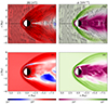 |
Fig. 1. Overview of the structure of the magnetosphere in Run1, on the meridian plane (top) and equatorial plane (bottom). Left: Module of the magnetic field. Right: Ion density. Both quantities were computed at a time of t = 11RM/vsw, x. |
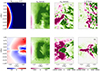 |
Fig. 2. Overview of the diffusion regions in Run1. From left to right: Out of plane magnetic field component, the ion velocity, electron velocity, and J ⋅ E, on the equatorial plane (top) and meridian (bottom). All quantities are computed at t = 3RM/vsw, x. |
As a first step, we study how the topology of the magnetic field lines affects the spatial distribution of the electrons. We split the domain according to the magnetic topology: those corresponding to magnetic field lines closed at both ends on the planet; those closed at one end; and, finally, the magnetically open ones. For each of these regions, we look at the distribution of electrons as a function of temperature. After the onset of magnetic reconnection at t ∼ 2RM/vsw, x, an increase of electron energy is observed. High-energy electrons, initially equally spread in the three topological regions eventually only become visible in magnetic closed regions, as they are trapped. In Fig. 3, we show the distribution of electrons for temperatures greater than 100 eV (top) and 1 keV (bottom), in the reconnection meridian plane, averaging along the out-of-plane direction, at t = 11RM/vsw, x. The figure has been realized by plotting the number of cells with electron temperature over the considered threshold.
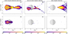 |
Fig. 3. Histograms of the number of cells in Run1 for which the electron temperature is above 100 eV (top) and 1 KeV (bottom), in the meridian plane, averaging along the out-of-plane direction, in the magnetic field region closed with the planet (left), open with respect to the planet (right) and with one open and one closed extremity (center), in the meridian plane, averaging along the out-of-plane direction. Quantities computed at t = 11RM/vsw, x. |
We observe that for energies below 1 KeV, electrons are almost equally distributed in the three different regions (subplots a, b, and c). Considering energetic electrons (with temperatures over the Kev) they are only found in regions with magnetic field lines closed on the planet (d), while no energetic electrons are observed in regions with one-side (e) or completely open (f) magnetic field. These results indicate a clear link between magnetic topology and electron energy distribution. This can be explained by the fact that energetic particles stay trapped in the closed regions, while those in open field regions (also on just one side) escape the simulation domain and, therefore, the planetary environment. Moreover, in Fig. 4 we show the distribution of electrons trapped in the closed magnetic field regions, for energies above 100 eV (a) and 1 KeV (b). In Fig. 4, we observe an asymmetry between positive and negative y, in both energy ranges. Concerning the region behind the planet for −2 < x < −4, we observe that this asymmetry aligns with the density asymmetry that is also observed in Fig. 1. Specifically, lower particle densities are observed for negative y (see the dawn side of the magnetosphere, local time around 6 h). This result is consistent with what was previously observed and discussed in Lavorenti et al. (2022) regarding the role of the loss-cone mechanism creating inhomogeneous distribution of high energy electrons inside the magnetosphere of Mercury. The evolution of the distribution in this plane can be observed in Video 1 (available online).
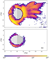 |
Fig. 4. Histograms of the number of cells in Run1 for which the electron temperature is above 100 eV (top) and 1 KeV (bottom), in the reconnection equatorial plane, averaging along the z direction, in the magnetic field region closed with the planet. Quantities are computed at t = 11RM/vsw, x. |
4. Whistler-mode waves in the magnetotail
On top of the magnetic reconnection dynamics, after t ∼ 4RM/vsw, x we observe waves developing nearby the X-point region in the magnetotail. These waves, observed until the end of the simulation, exhibit a narrow-band shape in the magnetic and electric fields, as well as in the electron current. In Fig. 5 we show in the x, z plane the magnetic field and perpendicular electric field (with respect to the magnetic field) fluctuations. The figure zooms at around the diffusion region where the waves are more intense and we over-plot the magnetic field lines to highlight the parallel propagation of the waves. These waves of relatively large amplitude originate from the diffusion region and propagate nearly parallel to the magnetic field, mainly along the separatrices, as shown in Fig. 5. The formation region and propagation direction of the waves can be even better observed in Video 2 (available online). These waves, in addition to the electromagnetic component, are also characterised by the presence of a strong electrostatic component E∥ and parallel electron current, as shown in Fig. 6. We also observe a small wave component in the ions current, albeit significantly smaller in magnitude.
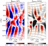 |
Fig. 5. Magnetic field (a) and electric field (b, perpendicular to the magnetic field) wave components, for t ∼ 11RM/vsw, x. Waves are in the plane at y = −0.5RM, where the waves features are clearer. Wave components are obtained by subtracting the mean field for both. Black lines are the magnetic field lines. |
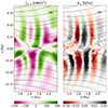 |
Fig. 6. Parallel electron current (a) and electric field (b) wave components, for t ∼ 11RM/vsw, x. Waves are in the plane at y = −0.5RM, where the waves features are clearer. Black lines are the magnetic field lines. |
In order to identify the mode, we have studied its polarization and dispersion relation. Concerning the polarization, these waves present a clear right-hand polarization. This is shown in Fig. 7, where we draw the hodogram in the perpendicular plane assuming the wave-vector as exactly parallel to the mean magnetic field.
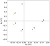 |
Fig. 7. Hodogram of the magnetic field components orthogonal to the wave vector B (assumed completely parallel to the magnetic field), at x = −2RM and z = −0.4RM. Each point correspond to a different time-step, with a cadence of |

Concerning the dispersion relation, we collected the outputs with a time step of  in order to well resolve the wave oscillation. Here, the sw and loc indices mean that the frequencies are computed in solar wind and locally averaged units, respectively. We observe narrow-band mode has a wave-vector kdi, loc ∼ 14 and an angular velocity ω ∼ 0.5ωce, loc, where di is the ion inertial length and ωce is the electron cyclotron frequency. Quantities in local unities are obtained by averaging the density and the magnetic field in the region over which the dispersion relation is computed. The range of frequencies and features proper of the mode correspond well to whistler waves.
In Fig. 8, where we draw the dispersion relation of the mode obtained by a Fourier transform in space and time. In this figure, we over-plot the dispersion relation for a whistler-mode wave propagating along the magnetic field in a cold plasma (Stix 1992; Omura et al. 2008):
 (1)
(1)
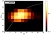 |
Fig. 8. Amplitude of the Fourier transform in both space and time of the observed waves compared with the theoretical dispersion relation for whistler waves (Eq. (1)). Quantities computed at t ∼ 11RM/vsw, x. |
We conclude that the observed mode is compatible with the whistler waves’ dispersion relation.
To better understand the nature of these waves, we investigated the electron anisotropy in the guise of the electron temperature anisotropy as a possible driver of whistler instability. In particular, the following condition is required (Kennel & Petschek 1966):
 (2)
(2)
In Fig. 9, we show the electron anisotropy (to which the wave contour is superimposed). In the figure, the red regions correspond to those where the condition in Eq. (2) is met. We observe that the threshold in Eq. (2) is reached locally around the reconnection region and closer to the planet. From Fig. 9, it is also seen that far from the reconnection region and along the separatrices, where the waves propagate, the parallel electron temperature is higher than the perpendicular one. As a result the waves are likely to be generated by the electron temperature anisotropy in the reconnection region. Interestingly, we observe that Te, ∥ > Te, ⊥ along the separatrices and further from the reconnection plane. In considering a possible nonlinear feedback of the generated whistler waves following a reduction of the electron temperature anisotropy, we compared the electron parallel thermal velocity with the whistler wave phase velocity. We observed that they differ by about two orders of magnitude. For this reason, we excluded the possibility that the parallel temperature increase along the separatrices is due to wave-particle interactions with the observed whistler waves. Instead, it is rather likely due to other processes within the diffusion region, such as electron parallel acceleration known to generate electron beams along the separatrices.
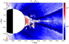 |
Fig. 9. Electron temperature anisotropy in the meridian plane, for t ∼ 11RM/vsw, x. Black lines are the contour plot of the waves, to indicate waves’ location. Red regions indicate where the condition in Eq. (2) is met. |
5. Discussion
In this study, we have presented two global numerical simulations of the Hermean magnetospheric environment. In particular, we have focused on magnetic reconnection at the magnetotail and its consequences on the energetic electron distribution. Moreover, around the diffusion region, waves at electron scales develop and propagate nearly parallel to the magnetic field.
First, we observe that magnetic reconnection in the magnetotail increases the electron temperature around the diffusion region. After reconnection onset, electrons below 1 keV are observed both in regions with open and closed magnetic field lines. Energetic electrons with energy above 1 KeV are instead only observed in regions with closed magnetic field lines since non-trapped electrons exit the simulation domain.
Second, the simulation reveals the presence of narrow-band whistler-mode waves in the magnetotail. These waves originate at the nightside reconnection site and propagate parallel to the magnetic field. Electron anisotropy has been identified to be the source of these waves. Furthermore, the region where the waves develop and propagate is characterized by an inhomogeneous plasma, with density and magnetic field magnitude varying by almost an order of magnitude. This strongly supports the notion that the background magnetic inhomogeneity plays a pivotal role in the generation process of planetary whistler waves, in agreement with the simulations modeling Mercury’s environment (Omura et al. 2008, 2015; Hikishima et al. 2009; Ozaki et al. 2023). The results shown in this work will be of crucial importance to interpret plasma waves observations by BepiColombo PWI instrument during the science phase.
It is worth discussing the possible role of the northward-shifted magnetic dipole of Mercury, observed from MESSENGER (Anderson et al. 2012), in the generation of the whistler waves we observe in the tail. In the specific numerical simulation reported in this paper, we did not use any shifted magnetic dipole moment. We have also run complementary numerical simulations that include the shift in Mercury’s magnetic dipole moment. The same waves as those reported here are observed in those simulations that include a dipole offset. Therefore, the existence of these waves near the reconnection point is found to be a general feature common to all mini-magnetospheres, rather than being specific to Mercury. Therefore, the results reported in this work extend beyond the study of planet Mercury.
Whistler-mode chorus waves have been observed during the two flybys at Mercury by BepiColombo (Ozaki et al. 2023). As discussed in this paper, obtaining a comprehensive global map of chorus waves on Mercury holds significant importance in comprehending the energetic electron loss mechanisms. In particular, our results may provide an early example of the distribution of such waves in the magnetotail. The location of the waves is shown in Fig. 10. Our results indicate that the waves propagate within low altitudes from the equatorial plane, at altitudes ranging from −1 to 1 RM, and that they are spread almost symmetrically with respect to the magnetic equatorial plane even if a bit more distributed dawnside. Nonetheless, BepiColombo measurements show the presence of whistler waves on the dawn side of Mercury, while they still have to be observed in the magnetotail region. In this study, we have considered only a purely southward IMF. To achieve a more comprehensive distribution map of such waves, it might be beneficial to investigate in the future how the location and the amplitude of these waves could be influenced by the upstream solar wind properties, especially the IMF direction.
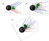 |
Fig. 10. Locations where the waves are observed at t ∼ 11RM/vsw, x. We show here the cells in Run1 for which the parallel component of the electric field is above a threshold of 26 mV/m, from three different perspectives. |
One of the characteristics of narrow-band whistler waves (i.e., the chorus) from observations and theory is “chirping”, consisting in the variation of the center frequency of the narrow-band wave as a function of time (Burtis & Helliwell 1969; Tsurutani & Smith 1974). In our simulations, however, this phenomenon was not observed. We do not know whether this is due to an absence of the phenomenon itself or to the total integration time of the simulation (because of computational reasons) not sufficient to let the chirping mechanism develop. Therefore, we refer to the observed waves as narrowband whistler waves. Nonetheless, the BepiColombo observations did not show the finer structures of typical rising-tone elements in the time domain due to telemetry limitations (Ozaki et al. 2023).
It is crucial to emphasize that in this scenario, the scaling of the planet could impact the waves’ location. This is primarily due to the proximity of the diffusion region to the planet, with the wavelength being comparable with the planet’s radius size. Indeed, due to computational constraints it still remains necessary to reduce the scale separation between planet, ion, and electron scales. Reducing the ion-to-electron mass ratio and the plasma-to-cyclotron frequency ratio is a well-established technique in fully kinetic simulations. Previous studies (Bret & Dieckmann 2010; Le et al. 2013; Lavorenti et al. 2021, 2022, 2023) have extensively discussed the effects of this approach.
Concerning the planet scaling, its influence on magnetic reconnection has already been discussed in Lavorenti et al. (2022, 2023). When the planet’s radius is scaled down (here, RM = 230 km and RM, 2 = 115 km, as opposed to the realistic radius of Mercury at about 2400 km), the diffusion regions in the tail, both for electrons and ions, moves closer to the planet’s surface. As shown in Fig. 1, there is a moderate separation of the ion and electron diffusion regions from the planet. Consequently, the ion dynamics within the outflow will be influenced by this reduction in size, but such an effect should not be observed for electrons. In particular, the characteristics of high-energy electrons observed in our simulations as a result of magnetic reconnection will remain consistent when dealing with a planet of actual size. Finally, comparing the modes that are generated in Run1 and Run2, we observe that the dispersion relation is not altered by scaling the planet.
6. Conclusions
We present the results of two global full-PIC numerical simulations of the Hermean magnetosphere addressing the development of magnetic reconnection and related dynamics at the magnetotail, in particular, focusing on the study of narrow band whistler waves originating around the reconnection region. These waves, driven by electron temperature anisotropy, propagate parallel to the magnetic field with a frequency of f ∼ 0.5fce, presenting both electromagnetic and electrostatic components. The possibility of studying these waves and their spatial distribution in the tail is of great importance to attain a better understanding of the electron dynamics in Mercury. Presently, the distinction in the spatio-temporal distribution of electron-driven chorus and whistler waves between Earth and Mercury remains unknown through observational means. Unraveling the distinctions between these two environments constitutes a forthcoming challenge, essential for stepping forward our comprehension of how solar wind shapes diverse planetary environments. To address this, the outcomes of the current study play a crucial role in designing and planning the forthcoming observations for the science phase subsequent to the final orbit insertion of BepiColombo in 2025.
Movies
Movie 1 (Video1) Access Supplementary Material
Movie 2 (Video2) Access Supplementary Material
Acknowledgments
This work was granted access to the HPC resources at TGCC under the allocations AP010412622 and A0100412428 made by GENCI via the DARI procedure. We acknowledge the Italian supercomputing center CINECA where the simulation has been performed under ISCRA grant. We acknowledge the support of CNES for the BepiColombo mission.
References
- Aizawa, S., Griton, L., Fatemi, S., et al. 2021, Planet. Space Sci., 198, 105176D [NASA ADS] [CrossRef] [Google Scholar]
- Allison, H. J., Shprits, Y. Y., Zhelavskaya, I. S., Wang, D., & Smirnov, A. G. 2021, Sci. Adv., 7, eabc0380 [NASA ADS] [CrossRef] [Google Scholar]
- Anderson, B. J., Johnson, C. L., Korth, H., et al. 2012, J. Geophys. Res. (Planets), 117, E00L12 [Google Scholar]
- Benkhoff, J., Murakami, G., Baumjohann, W., et al. 2021, Space Sci. Rev., 217, 90 [NASA ADS] [CrossRef] [Google Scholar]
- Benna, M., Anderson, B. J., Baker, D. N., et al. 2010, Icarus, 209, 3 [NASA ADS] [CrossRef] [Google Scholar]
- Biskamp, D., Schwarz, E., & Drake, J. F. 1997, Phys. Plasmas, 4, 1002 [CrossRef] [Google Scholar]
- Bret, A., & Dieckmann, M. E. 2010, Phys. Plasmas, 17, 032109 [NASA ADS] [CrossRef] [Google Scholar]
- Burtis, W. J., & Helliwell, R. A. 1969, J. Geophys. Res., 74, 3002 [CrossRef] [Google Scholar]
- Chen, Y., Tóth, G., Jia, X., et al. 2019, J. Geophys. Res. (Space Phys.), 124, 8954 [NASA ADS] [CrossRef] [Google Scholar]
- Cuesta, M. E., Chhiber, R., Roy, S., et al. 2022, ApJ, 932, L11 [NASA ADS] [CrossRef] [Google Scholar]
- Dibraccio, G. A., Slavin, J. A., Boardsen, S. A., et al. 2013, J. Geophys. Res. (Space Phys.), 118, 997 [NASA ADS] [CrossRef] [Google Scholar]
- DiBraccio, G. A., Slavin, J. A., Raines, J. M., et al. 2015, Geophys. Res. Lett., 42, 9666 [NASA ADS] [CrossRef] [Google Scholar]
- Dong, C., Wang, L., Hakim, A., et al. 2019, Geophys. Res. Lett., 46, 584 [NASA ADS] [Google Scholar]
- Drake, J. F., & Kleva, R. G. 1991, Phys. Rev. Lett., 66, 1458 [NASA ADS] [CrossRef] [Google Scholar]
- Dungey, J. W. 1961, Phys. Rev. Lett., 6, 47 [NASA ADS] [CrossRef] [Google Scholar]
- Exner, W. 2021, Ph.D. Thesis, Modeling of Mercury’s Magnetosphere Under Different Solar Wind Conditions [Google Scholar]
- Exner, W., Heyner, D., Liuzzo, L., et al. 2018, Planet. Space Sci., 153, 89 [NASA ADS] [CrossRef] [Google Scholar]
- Exner, W., Simon, S., Heyner, D., & Motschmann, U. 2020, J. Geophys. Res. (Space Phys.), 125, e2019JA027691 [CrossRef] [Google Scholar]
- Fatemi, S., Poirier, N., Holmström, M., et al. 2018, A&A, 614, A132 [NASA ADS] [CrossRef] [EDP Sciences] [Google Scholar]
- Fujimoto, M., Shinohara, I., & Kojima, H. 2011, Space Sci. Rev., 160, 123 [CrossRef] [Google Scholar]
- Fuselier, S. A., Vines, S. K., Burch, J. L., et al. 2017, J. Geophys. Res. (Space Phys.), 122, 5466 [CrossRef] [Google Scholar]
- Glauert, S. A., & Horne, R. B. 2005, J. Geophys. Res. (Space Phys.), 110, 2004JA010851 [NASA ADS] [CrossRef] [Google Scholar]
- Gurnett, D. A., Kurth, W. S., Scarf, F. L., & Poynter, R. L. 1986, Science, 233, 106 [NASA ADS] [CrossRef] [Google Scholar]
- Gurnett, D. A., Shaw, R. R., Anderson, R. R., Kurth, W. S., & Scarf, F. L. 1979, Geophys. Res. Lett., 6, 511 [NASA ADS] [CrossRef] [Google Scholar]
- Hikishima, M., Yagitani, S., Omura, Y., & Nagano, I. 2009, J. Geophys. Res. (Space Phys.), 114, 1203 [Google Scholar]
- Horne, R. B., Thorne, R. M., Shprits, Y. Y., et al. 2005, Nature, 437, 227 [NASA ADS] [CrossRef] [Google Scholar]
- Horne, R. B., Thorne, R. M., Glauert, S. A., et al. 2008, Nat. Phys., 4, 301 [CrossRef] [Google Scholar]
- Hua, M., Bortnik, J., & Ma, Q. 2022, Geophys. Res. Lett., 49, e2022GL099618 [CrossRef] [Google Scholar]
- Hua, M., Bortnik, J., Kellerman, A. C., Camporeale, E., & Ma, Q. 2023, Space Weather, 21, e2022SW003234 [NASA ADS] [CrossRef] [Google Scholar]
- Imber, S. M., Slavin, J. A., Boardsen, S. A., et al. 2014, J. Geophys. Res. (Space Phys.), 119, 5613 [NASA ADS] [CrossRef] [Google Scholar]
- Ip, W.-H., & Kopp, A. 2002, J. Geophys. Res. (Space Phys.), 107, SSH 4 [Google Scholar]
- James, M. K., Imber, S. M., Bunce, E. J., et al. 2017, J. Geophys. Res. (Space Phys.), 122, 7907 [NASA ADS] [CrossRef] [Google Scholar]
- Jia, X., Slavin, J. A., Gombosi, T. I., et al. 2015, J. Geophys. Res. (Space Phys.), 120, 4763 [NASA ADS] [CrossRef] [Google Scholar]
- Jia, X., Slavin, J. A., Poh, G., et al. 2019, J. Geophys. Res. (Space Phys.), 124, 229 [NASA ADS] [CrossRef] [Google Scholar]
- Kabin, K. 2000, Icarus, 143, 397 [NASA ADS] [CrossRef] [Google Scholar]
- Kallio, E., & Janhunen, P. 2003, Ann. Geophys., 21, 2133 [NASA ADS] [CrossRef] [Google Scholar]
- Kallio, E., & Janhunen, P. 2004, Adv. Space Res., 33, 2176 [NASA ADS] [CrossRef] [Google Scholar]
- Kasaba, Y., Kojima, H., Moncuquet, M., et al. 2020, Space Sci. Rev., 216, 65 [NASA ADS] [CrossRef] [Google Scholar]
- Kennel, C. F., & Petschek, H. E. 1966, J. Geophys. Res., 71, 1 [NASA ADS] [CrossRef] [Google Scholar]
- Khotyaintsev, Y. V., Graham, D. B., Norgren, C., & Vaivads, A. 2019, Front. Astron. Space Sci., 6, 70 [NASA ADS] [CrossRef] [Google Scholar]
- Kurth, W. S., & Gurnett, D. A. 1991, J. Geophys. Res. (Space Phys.), 96, 18977 [CrossRef] [Google Scholar]
- Lapenta, G., Schriver, D., Walker, R. J., et al. 2022, J. Geophys. Res. (Space Phys.), 127, e2021JA030241 [CrossRef] [Google Scholar]
- Lauben, D. S., Inan, U. S., Bell, T. F., et al. 1998, Geophys. Res. Lett., 25, 2995 [CrossRef] [Google Scholar]
- Lavorenti, F. 2023, Mercury Particle Precipitation using Full-PIC Global Simulations [Google Scholar]
- Lavorenti, F., Henri, P., Califano, F., Aizawa, S., & André, N. 2021, A&A, 652, A20 [NASA ADS] [CrossRef] [EDP Sciences] [Google Scholar]
- Lavorenti, F., Henri, P., Califano, F., et al. 2022, A&A, 664, A133 [NASA ADS] [CrossRef] [EDP Sciences] [Google Scholar]
- Lavorenti, F., Henri, P., Califano, F., et al. 2023, A&A, 674, A153 [NASA ADS] [CrossRef] [EDP Sciences] [Google Scholar]
- Le, A., Egedal, J., Ohia, O., et al. 2013, Phys. Rev. Lett., 110, 135004 [NASA ADS] [CrossRef] [Google Scholar]
- Le Contel, O., Roux, A., Jacquey, C., et al. 2009, Ann. Geophys., 27, 2259 [NASA ADS] [CrossRef] [Google Scholar]
- Liu, K., Gary, S. P., & Winske, D. 2011, Geophys. Res. Lett., 38, L14108 [Google Scholar]
- Mandt, M. E., Denton, R. E., & Drake, J. F. 1994, Geophys. Res. Lett., 21, 73 [CrossRef] [Google Scholar]
- Markidis, S., Lapenta, G., & Rizwan-uddin, 2010, Math. Comput. Simul., 80, 1509 [CrossRef] [Google Scholar]
- Milillo, A., Fujimoto, M., Murakami, G., et al. 2020, Space Sci. Rev., 216, 93 [NASA ADS] [CrossRef] [Google Scholar]
- Müller, J., Simon, S., Wang, Y.-C., et al. 2012, Icarus, 218, 666 [CrossRef] [Google Scholar]
- Ness, N. F., Behannon, K. W., Lepping, R. P., Whang, Y. C., & Schatten, K. H. 1974, Science, 185, 151 [NASA ADS] [CrossRef] [Google Scholar]
- Ness, N. F., Behannon, K. W., Lepping, R. P., & Whang, Y. C. 1976, Icarus, 28, 479 [NASA ADS] [CrossRef] [Google Scholar]
- Nogi, T., Nakamura, S., & Omura, Y. 2020, J. Geophys. Res. (Space Phys.), 125, e2020JA027953 [CrossRef] [Google Scholar]
- Oliven, M. N., & Gurnett, D. A. 1968, J. Geophys. Res., 73, 2355 [NASA ADS] [CrossRef] [Google Scholar]
- Omura, Y., Katoh, Y., & Summers, D. 2008, J. Geophys. Res. (Space Phys.), 113, 4223O [CrossRef] [Google Scholar]
- Omura, Y., Miyashita, Y., Yoshikawa, M., et al. 2015, J. Geophys. Res. (Space Phys.), 120, 9545 [CrossRef] [Google Scholar]
- Ozaki, M., Yagitani, S., Kasaba, Y., et al. 2023, Nat. Astron., 7, 11 [Google Scholar]
- Pantellini, F., Griton, L., & Varela, J. 2015, Planet. Space Sci., 112, 1 [NASA ADS] [CrossRef] [Google Scholar]
- Poh, G., Slavin, J. A., Jia, X., et al. 2017, Geophys. Res. Lett., 44, 678 [NASA ADS] [CrossRef] [Google Scholar]
- Raines, J. M., DiBraccio, G. A., Cassidy, T. A., et al. 2015, Space Sci. Rev., 192, 91 [NASA ADS] [CrossRef] [Google Scholar]
- Russell, C. T., Baker, D. N., & Slavin, J. A. 1988, The Magnetosphere of Mercury, 113, 4223O [Google Scholar]
- Sarantos, M., Killen, R. M., & Kim, D. 2007, Planet. Space Sci., 55, 1584 [NASA ADS] [CrossRef] [Google Scholar]
- Scarf, F. L., Gurnett, D. A., & Kurth, W. S. 1979, Science, 204, 991 [NASA ADS] [CrossRef] [Google Scholar]
- Scudder, J., & Daughton, W. 2008, J. Geophys. Res. (Space Phys.), 113, A06222 [Google Scholar]
- Siscoe, G. L., Ness, N. F., & Yeates, C. M. 1975, J. Geophys. Res., 80, 4359 [CrossRef] [Google Scholar]
- Slavin, J. A. 2004, Adv. Space Res., 33, 1859 [NASA ADS] [CrossRef] [Google Scholar]
- Slavin, J. A., Anderson, B. J., Zurbuchen, T. H., et al. 2009, Geophys. Res. Lett., 36, L02101 [Google Scholar]
- Slavin, J. A., Anderson, B. J., Baker, D. N., et al. 2012, J. Geophys. Res. (Space Phys.), 117, A01215 [NASA ADS] [Google Scholar]
- Slavin, J. A., DiBraccio, G. A., Gershman, D. J., et al. 2014, J. Geophys. Res. (Space Phys.), 119, 8087 [CrossRef] [Google Scholar]
- Slavin, J. A., Middleton, H. R., Raines, J. M., et al. 2019, J. Geophys. Res. (Space Phys.), 124, 6613 [CrossRef] [Google Scholar]
- Solomon, S. C., & Anderson, B. J. 2018, The View after MESSENGER, eds. S. C. Solomon, L. R. Nittler, & B. J. Anderson, 1 [Google Scholar]
- Spreiter, J. R., Summers, A. L., & Alksne, A. Y. 1966, Planet. Space Sci., 14, 223 [NASA ADS] [CrossRef] [Google Scholar]
- Stix, T. 1992, Waves in Plasmas, 566 [Google Scholar]
- Summers, D., Thorne, R. M., & Xiao, F. 1998, J. Geophys. Res. (Space Phys.), 103, 20487 [NASA ADS] [CrossRef] [Google Scholar]
- Summers, D., Ni, B., & Meredith, N. P. 2007, J. Geophys. Res. (Space Phys.), 112, A4 [Google Scholar]
- Sun, W. J., Fu, S. Y., Slavin, J. A., et al. 2016, J. Geophys. Res. (Space Phys.), 121, 7590 [CrossRef] [Google Scholar]
- Sundberg, T., Slavin, J. A., Boardsen, S. A., et al. 2012, J. Geophys. Res. (Space Phys.), 117, A00M03 [NASA ADS] [Google Scholar]
- Thorne, R. M., Li, W., Ni, B., et al. 2013, Nature, 504, 411 [NASA ADS] [CrossRef] [Google Scholar]
- Trávníček, P., Hellinger, P., & Schriver, D. 2007, Geophys. Res. Lett., 34, L05104 [Google Scholar]
- Trávníček, P. M., Hellinger, P., Schriver, D., et al. 2009, Geophys. Res. Lett., 36, L07104 [Google Scholar]
- Trávníček, P. M., Schriver, D., Hellinger, P., et al. 2010, Icarus, 209, 11 [CrossRef] [Google Scholar]
- Tsurutani, B. T., & Smith, E. J. 1974, J. Geophys. Res., 79, 118 [CrossRef] [Google Scholar]
- Winslow, R. M., Anderson, B. J., Johnson, C. L., et al. 2013, J. Geophys. Res. (Space Phys.), 118, 2213 [NASA ADS] [CrossRef] [Google Scholar]
- Woodfield, E. E., Glauert, S. A., Menietti, J. D., et al. 2019, Geophys. Res. Lett., 46, 7191 [NASA ADS] [CrossRef] [Google Scholar]
- Xiao, F., Yang, C., He, Z., et al. 2014, J. Geophys. Res. (Space Phys.), 119, 3325 [NASA ADS] [CrossRef] [Google Scholar]
- Yagi, M., Seki, K., Matsumoto, Y., Delcourt, D. C., & Leblanc, F. 2010, J. Geophys. Res. (Space Phys.), 115, A10 [Google Scholar]
- Yu, X., Yuan, Z., Li, H., et al. 2018, Geophys. Res. Lett., 45, 8755 [NASA ADS] [CrossRef] [Google Scholar]
All Tables
All Figures
|
Fig. 1. Overview of the structure of the magnetosphere in Run1, on the meridian plane (top) and equatorial plane (bottom). Left: Module of the magnetic field. Right: Ion density. Both quantities were computed at a time of t = 11RM/vsw, x. |
| In the text | |
|
Fig. 2. Overview of the diffusion regions in Run1. From left to right: Out of plane magnetic field component, the ion velocity, electron velocity, and J ⋅ E, on the equatorial plane (top) and meridian (bottom). All quantities are computed at t = 3RM/vsw, x. |
| In the text | |
|
Fig. 3. Histograms of the number of cells in Run1 for which the electron temperature is above 100 eV (top) and 1 KeV (bottom), in the meridian plane, averaging along the out-of-plane direction, in the magnetic field region closed with the planet (left), open with respect to the planet (right) and with one open and one closed extremity (center), in the meridian plane, averaging along the out-of-plane direction. Quantities computed at t = 11RM/vsw, x. |
| In the text | |
|
Fig. 4. Histograms of the number of cells in Run1 for which the electron temperature is above 100 eV (top) and 1 KeV (bottom), in the reconnection equatorial plane, averaging along the z direction, in the magnetic field region closed with the planet. Quantities are computed at t = 11RM/vsw, x. |
| In the text | |
|
Fig. 5. Magnetic field (a) and electric field (b, perpendicular to the magnetic field) wave components, for t ∼ 11RM/vsw, x. Waves are in the plane at y = −0.5RM, where the waves features are clearer. Wave components are obtained by subtracting the mean field for both. Black lines are the magnetic field lines. |
| In the text | |
|
Fig. 6. Parallel electron current (a) and electric field (b) wave components, for t ∼ 11RM/vsw, x. Waves are in the plane at y = −0.5RM, where the waves features are clearer. Black lines are the magnetic field lines. |
| In the text | |
|
Fig. 7. Hodogram of the magnetic field components orthogonal to the wave vector B (assumed completely parallel to the magnetic field), at x = −2RM and z = −0.4RM. Each point correspond to a different time-step, with a cadence of |
| In the text | |
|
Fig. 8. Amplitude of the Fourier transform in both space and time of the observed waves compared with the theoretical dispersion relation for whistler waves (Eq. (1)). Quantities computed at t ∼ 11RM/vsw, x. |
| In the text | |
|
Fig. 9. Electron temperature anisotropy in the meridian plane, for t ∼ 11RM/vsw, x. Black lines are the contour plot of the waves, to indicate waves’ location. Red regions indicate where the condition in Eq. (2) is met. |
| In the text | |
|
Fig. 10. Locations where the waves are observed at t ∼ 11RM/vsw, x. We show here the cells in Run1 for which the parallel component of the electric field is above a threshold of 26 mV/m, from three different perspectives. |
| In the text | |
Current usage metrics show cumulative count of Article Views (full-text article views including HTML views, PDF and ePub downloads, according to the available data) and Abstracts Views on Vision4Press platform.
Data correspond to usage on the plateform after 2015. The current usage metrics is available 48-96 hours after online publication and is updated daily on week days.
Initial download of the metrics may take a while.