© The Authors 2023

1. Introduction

In young stellar objects (YSOs) such as young T-Tauri stars, the process of accretion of material from the initial cloud is almost complete and the star is just about to start burning its thermonuclear fuel. During the gravitational infall of matter onto a central object, an accretion disk is formed, through which angular momentum is transported away from the central object.

To construct consistent stellar spin-down models of the formation of Sun-like stars, a magnetic field is required (Bouvier & Cébron 2015; Ahuir et al. 2020). Apart from the stellar wind properties, a self-consistent treatment of star-disk magnetospheric interaction need to be included in the considerations. Analytical solutions for magnetic thin accretion disks are impossible without imposing severe approximations because the system of equations is not closed (Čemeljić et al. 2019). This leaves us with self-consistent numerical simulations as the only way to obtain a solution. Important steps have been undertaken by Ghosh & Lamb (1979a,b), who found that to correctly describe the star-disk magnetospheric interaction, it is necessary to include the rotating stellar surface and corona as well as to extend the computational domain beyond the position of the corotation radius. Matt & Pudritz (2005), Matt et al. (2012) discussed spin-down models and the dependence of torque on stellar field stellar rotation rates. In a series of works, Romanova et al. (2009, 2013) investigated the star-disk interaction in numerical simulations, as did Zanni & Ferreira (2009, 2013), Čemeljić (2019). These authors identified the typical geometry in simulations, with the magnetospheric wind, disk accretion flow, accretion column onto the central object, and (in cases where there is less magnetic diffusion in the disk) magnetospheric ejections.

Global numerical solutions describing the effect of magnetic field (in particular, resistivity) on the transport of angular momentum in the star-disk magnetosphere are still overly dependent on the chosen parameters in the disk. The torques caused by the stellar wind and ejection are not enough to counterbalance the torque exerted onto the central object by the material accreted through the disk. Also, the influence of magnetic reconnection in the disk corona remains undetermined.

There has not yet been any numerical simulations study that would extensively relate the quantities of (turbulent) resistive magnetohydrodynamics (MHD) in the disk and star-disk magnetospheric interaction as we do here. For comparisons with the observational data, a study in a large part of parameter space is needed. Such a study will yield trends; namely: expressions that are proportional to the dependence of various components of torques on density, velocity, and magnetic field components, as well as on the effective (anomalous) coefficients of both viscosity and resistivity.

Prescriptions from models, such as those given in Gallet et al. (2019), match the observed quantities reasonably well, but they do depend on the chosen limits of validity for each phase of pre-stellar evolution and require unrealistic large stellar fields to counterbalance the disk accretion for the spinning-up a star. Alternatively, a large mass loads in the stellar wind of up to 10% accretion rate are needed or, otherwise, an interplay of the lighter stellar wind with the disk truncation near the corotation radius. Consequently, more realistic models, informed by relevant numerical simulations, are needed to remove the implicit model requirements.

A comparison of the results from our numerical simulations with the results from models as given in Gallet et al. (2019) can serve both as a guide in evaluation of the simulations results and as information for the further refinements of the model. Following Zanni & Ferreira (2009), in Čemeljić (2019) we set a Kluzniak & Kita (2000, hereafter KK00) disk as the initial condition in our simulations, adding the stellar dipole magnetic field. We obtained an “atlas” of magnetic solutions, with three types of solutions for the slowly rotating star: with and without the accretion column, and with a magnetospheric ejection above the accretion column. An initial parameter study was performed in the 64 cases with different magnetic field strengths, stellar rotation rates and (anomalous) resistivity parameters. We found continuous trends in the average angular momentum flux transported onto the stellar surface through the accretion column from the disk onto the star. We also found a trend in the angular momentum flux expelled from the system in the magnetospheric ejection, which forms in the solutions with the resistive coefficient α_m = 0.1 in our simulations. Here, we describe the subsequent analysis of our 64 runs.

In the present study, contributions in the accretion flow onto the star are decomposed by the torque they exert on the stellar surface. Any speeding up or slowing down of the stellar rotation depends precisely upon the distance separating the field lines from the star to their footpoint anchoring in the disk. We also indicate trends in the torque exerted on a star by the magnetospheric ejection and stellar wind, and we check for trends in the total torque in the system with respect to the stellar magnetic field, stellar rotation rate, and resistivity.

In Sect. 2, we briefly present our numerical setup and give a general overview of the obtained quasi-stationary states and flows. Trends in the reach of stellar magnetic field in the disk are outlined in Sect. 3. In Sect. 4, we present the details of our computation of torques from the different components in the star-disk system and present the obtained trends in Sect. 5. We give our conclusions in Sect. 6.

2. Short overview of simulations

Similar simulations were previously reported in Romanova et al. (2009) with their (not publicly available) code and in Zanni & Ferreira (2009, 2013) with the (publicly available) PLUTO code (v.3) by Mignone et al. (2007). Our simulations in Čemeljić et al. (2017) were the first to repeat the latter setup, with the updated version of the PLUTO code (v.4.1) and minor amendments, as detailed in the appendix in Čemeljić (2019). We used the same resolution and choice of parameters to make sure we can make a direct comparison in the parameter study with the results obtained in the previous publications by Zanni & Ferreira (2009, 2013).

We performed 64 star-disk magnetospheric interaction simulations in a setup detailed in a spherical 2D axisymmetric grid in a physical domain from the stellar surface to 30 stellar radii. The resolution is at (R × θ) = (217 × 100) grid cells, with a logarithmic radial and uniform meridional distribution of grid cells. We performed simulations in a quadrant of θ ∈ [0, π/2], with the assumption of the equatorial symmetry. The initial disk was set by the KK00 solution, with a non-rotating corona in hydrostatic equilibrium. The viscosity coefficient was always set to α_v = 1, to avoid solutions with a midplane backflow; in the analytical solution given in KK00, backflow appears in the cases with viscous α parameter smaller than a critical value of 0.685. Solutions with a midplane backflow we presented separately in Mishra et al. (2020b,c, 2023).

After a few tens of stellar rotations, the system relaxes from the initial and boundary conditions, and reaches the quasi-stationary state. Examples of our results, showing the disk and its corona with the accretion column and the magnetospheric ejection (“conical wind” in Romanova et al. 2009 or “conical outflow” in Čemeljić 2019) are shown in Fig. 1.

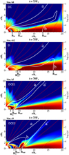Fig. 1. Four typical geometries in our solutions: Disk+Column (DC), Disk (D), Disk+Column+Ejection1 (DCE1), and Disk+Column+Ejection2 (DCE2) illustrated by snapshots in quasi-stationary states in simulations b8, d12, b5, and c9 (top to bottom, respectively). We show the density in a logarithmic color grading, with a sample of magnetic field lines in red solid lines. White lines labeled a, a’, b, and c delimit the components of the flow between which we integrate the fluxes; Rin, Rout and Rcor are the inner disk edge, the furthest outer reach of closed stellar field in the disk and the corotation radius, respectively.

In our simulations, we systematically explored the parameter space shown in Table 1, with slowly rotating star, up to 20% of the stellar breakup rotation rate ${\mathrm{\Omega }}_{\mathrm{br}}=\sqrt{G{M}_{\star }/R_{\star }^3}$. In the case of YSOs, the probed stellar rotation periods were in the range of 2–9 days, with the corresponding corotation radii $R_{\text{cor}}={(G{M}_{\star }/{\mathrm{\Omega }}_{\star }^2)}^{1/3}\sim 3-7$ stellar radii (see Table 1 in Čemeljić 2019). The second parameter we varied was the stellar dipole magnetic field strength at the stellar equator, B_⋆, which can take values from 250–1000 Gauss¹. This makes our choice of field strengths twice larger then expected fields observed in the YSO cases. This does not change our conclusions: in our simulations shift to smaller strengths of magnetic field preserves the trends well, numerical problems arise with larger fields. The third varying parameter was the anomalous resistivity coefficient, α_m, in the disk, which we set to values ranging from 0.1 to 1.

With regard to the geometry of the solution and position of lines across which we perform the integration of angular momentum and mass fluxes, the obtained solutions can be divided into the three cases as shown in Fig. 2 in Čemeljić (2019). For the reasons of additional analysis, here we distinguish the results with magnetospheric ejections by the position of the radius at which the ejection is launched: below or beyond the corotation radius, resulting in four different states, as shown in Fig. 1.

We exemplify the four distinct types of solutions with the representative simulations. In the simulation b8 shown in the top panel of Fig. 1 we obtain a disk and accretion column. With a faster rotating star and larger magnetic field in the simulation d12, the disk is pushed away from the star and there is no accretion column-it is a disk only solution, a “propeller” regime (Illarionov & Sunyaev 1975; Lovelace et al. 1999). These two cases echo a cartoon in Matt & Pudritz (2005; Fig. 3 in that work), which we also find in simulations. In the two bottom panels are shown results with α_m = 0.1, where in addition to the disk and accretion column, we obtain magnetospheric ejection: in the simulation b5 it is launched from below R_cor, and in simulation c9 beyond R_cor.

Each of our 64 results can be presented as one of the four cases described above, as shown in Fig. 1:

• DC: (Disk+column) The disk inner radius and accretion column are both positioned below the corotation radius. Stellar magnetic field lines are anchored well beyond the corotation radius, R_out > R_cor.

• D: (Disk) With faster rotating star and larger magnetic field, the disk inner radius is pushed further away from the star, beyond the corotation radius, and the accretion column is not formed. This is the “propeller regime.” The field lines are anchored in the disk far away from the star, still enabling some inflow of matter onto the star, R_out > R_cor.

• DCE1: (Disk+Column+Ejection1) A disk truncation radius and accretion column are both positioned below the corotation radius, and a magnetospheric ejection is launched from the magnetosphere. Stellar field is not reaching beyond the corotation radius, R_out < R_cor.

• DCE2: (Disk+Column+Ejection2) The second type of solution with a magnetospheric ejection, with the disk truncation radius and accretion column positioned partly below, and partly beyond the corotation radius. In this case, stellar field is anchored beyond the corotation radius, R_out > R_cor, but just beyond the accretion column footpoint in the disk.

The results with the different parameters are given in Table 2 in Čemeljić (2019). With the new distinction, in cases with magnetospheric ejection, this table remains valid here; it is only the DCE cases that are split into DCE1 and DCE2 for the launching of the magnetospheric ejection below and beyond the corotation radius, respectively. We list the solutions in Table 1.

3. Reach of the stellar magnetic field in the disk

The characteristic radii which we can determine from our simulations are the inner disk radius, R_in, the corotation radius of the material in the disk with the stellar surface (at the equator), R_cor, and the anchoring radius of the furthest line of magnetic field connecting the disk with the stellar surface, R_out.

Different characteristic radii have been discussed in the star-disk interaction models, as, for instance, Matt & Pudritz (2005). In Fig. 2, we present our results for the position of R_out, where some trends can be recovered: R_out increases with the larger resistive coefficient α_m for all stellar magnetic fields. There are some significant departures from the trends, which are probably related to the details of the flow geometry: in the case with B_⋆ = 0.5 kG (shown in the right top panel in the same figure) the largest R_out is measured at the slowest stellar rotation rate, out of the trend for other magnetic field strengths. In the bottom panels in this figure are shown the inner disk radii, R_in, with the same parameters, showing similar trends with the resistivity coefficient, α_m, and stellar magnetic field.

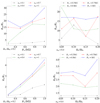Fig. 2. Positions of the anchoring radius, Rout, for the furthest stellar magnetic field line in the disk that still reaches the star and the inner disk radius, Rin. Top panels: Rout increases with the increasing resistive coefficient αm for all stellar magnetic fields (left) and position of the Rout as a function of stellar rotation rate in the cases without magnetospheric ejection shows a decreasing trend with the stellar magnetic field (right). It is only in the cases with B⋆ = 0.5 kG that we obtain a departure from this trend, with the largest Rout at the slowest stellar rotation rate. Bottom panels: Inner disk radius, Rin, is increasing in the majority of the cases with same parameters as in the above panels for Rout.

In all the cases with α_m = 0.1, a magnetospheric ejection is launched from the system in our simulations. In Fig. 3, it is shown that in such cases, there is only a minor dependence of R_out on the stellar rotation rates for all the stellar field strengths. Also, the increase of R_out with the stellar field strength is not large in such cases. We thus go on to consider why the magnetospheric ejections are launched only in cases where α_m = 0.1? With larger values of α_m, there is obviously enough magnetic diffusion to allow the matter to cross the magnetic field lines not to push them towards the star during accretion. When there is not enough dissipation, as with α_m = 0.1, the magnetic field lines will be pressed towards the star, where the mounting magnetic pressure pushes them away from the star, expelling some of matter in the magnetospheric ejections. The DCE2 type of solution from Fig. 1 (Sim. c9), pushed further in the magnetic field strength and with more magnetic diffusivity, would finish in the “propeller regime”, type D (Sim. d12).

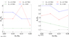Fig. 3. Variation of the furthest anchoring radius of the stellar field in the disk Rout with the stellar field in the cases with αm = 0.1 (which are all with a magnetospheric ejection launched from the system) is not large (left). Without the magnetospheric ejection, the scattering in this result is much larger. Inner disk radius Rin in the same cases displays a clear increasing trend with the increase of stellar magnetic field (right).

4. Torque exerted on a star

Next, we compute the torques applied on the star from the various components of the flow and magnetic field. The azimuthal magnetic field plays a key role in the torques computed, so in Fig. 4 we illustrate the behavior of B_φ with respect to the stellar rotation rate, based on the example of solutions without a magnetospheric ejection, with α_m = 1 and B_⋆ = 500 G. We find that B_φ atop the disk (top panel) is small and does not vary much in the cases with different Ω_⋆.

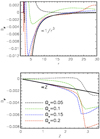Fig. 4. Toroidal magnetic field values along the disk surface (top) and along the disk height (measured from the disk equatorial plane) at R = 12R⋆ (bottom) are shown in terms of their dependence of stellar rotation rates. The values are averaged over 10 stellar rotation periods during the quasi-stationary states, in the cases with αm = 1 and B⋆ = 500 G (simulations b1, b5, b9, and b13). In black, green, blue, and red dashed lines we display the values for 0.05, 0.1, 0.15, and 0.2 of Ωbr, respectively. The black solid lines provide the reference for typical radial and vertical dependence.

The mass and angular momentum fluxes are obtained by integrating

$$\begin{array}{cc}\hfill \dot{M}& ={\displaystyle {\int }_{\mathrm{S}}\rho {\mathit{v}}_{\mathrm{p}}·\mathrm{d}\mathit{S},}\hfill \end{array}$$(1)

$$\begin{array}{cc}\hfill {\dot{J}}_{\mathrm{tot}}& ={\displaystyle {\int }_{\mathrm{S}}(r\rho v_{\phi }{\mathit{v}}_{\mathrm{p}}-\frac{r{B}_{\phi }{\mathit{B}}_{\mathrm{p}}}{4\pi })\mathrm{d}\mathit{S},}\hfill \end{array}$$(2)

where S is the surface of integration.

We computed the fluxes in each of the 64 simulations, to find trends in different combinations of parameters. Depending on the geometry of the solution, the boundaries of the integration change, as shown in Fig. 1. We discuss the possible configurations below.

First, the simplest configuration is with the disk and accretion column, which we find in majority of the simulations with the resistivity coefficient α_m > 0.1. Then, in cases with larger magnetic field and faster stellar rotation, we find that the disk is pushed away from the star, and the accretion column is disrupted. Finally, in cases with a magnetospheric ejection, there is an additional component in the flow, so we then modify the contours of integration.

The mass accretion rates are computed across the various surfaces. The mass load in the stellar wind is:

$$\begin{array}{c}\hfill {\dot{M}}_{\mathrm{SW}}=4\pi R_{\star }^2{\displaystyle {\int }_{{\theta }_{\mathrm{a}}}^0\rho v_{\mathrm{R}}sin\theta a\theta ,}\end{array}$$(3)

computed across the stellar surface. The accretion rate onto the stellar surface

$$\begin{array}{c}\hfill {\dot{M}}_{\star }=-4\pi R_{\star }^2{\displaystyle {\int }_{{\theta }_{\mathrm{b}}}^{\pi /2}\rho v_{\mathrm{R}}sin\theta \mathrm{d}\theta ,}\end{array}$$(4)

is also computed across the stellar surface. The θ_a refers to the angle of the last open magnetic surface and θ_b to the footpoint of the last closed line of magnetic flux b (see, e.g., the third panel in Fig. 1, for the DCE1 case). The disk accretion rate,

$$\begin{array}{c}\hfill {\dot{M}}_{\mathrm{d}}=-4\pi R^2{\displaystyle {\int }_{{\theta }_{\mathrm{b}}}^{\pi /2}\rho v_{\mathrm{R}}sin\theta \mathrm{d}\theta ,}\end{array}$$(5)

is computed at R = 12R_⋆, the same as mass load in the magnetospheric ejection,

$$\begin{array}{c}\hfill {\dot{M}}_{\mathrm{out}}=4\pi R^2{\displaystyle {\int }_{{\theta }_{{\mathrm{a}}^{\prime }}}^{{\theta }_{\mathrm{a}}}\rho v_{\mathrm{R}}sin\theta \mathrm{d}\theta ,}\end{array}$$(6)

where θ_disk is the angle at which is the disk surface, θ_a and θ_a′ are the angles encompassing the magnetospheric ejection², as shown in Fig. 1. The different distances at which the mass fluxes are computed for separate components in the flow render the sum for the total mass flux elusive, as some of the mass flux is mixed between the components between the stellar surface and R = 12R_⋆. The relative discrepancy in the mass accretion rate in the disk and the sum of the mass fluxes in our results, (Ṁ_d − Ṁ_SW − Ṁ_⋆ − Ṁ_out)/Ṁ_d, measures this mixing. In most of our cases the relative discrepancy is low, below 10%. In the cases with violent reconnection when the flow is severely disrupted at some locations during the run, or with some other instability, it can grow, up to few tens of percents. This is probably the reason for some of the outliers in the trends for mass fluxes. In the subsections in Sect. 5, we show that mass fluxes enter the (approximate) analytical solutions for torques, through the coefficients of proportionality in the expressions for different characteristic radii. To better capture the different physical regimes in the flows, a separation of the results from our simulations in more sub-groups would probably be needed. We leave this aspect for a future study.

The torque from the stellar surface into the stellar wind³, ${\dot{J}}_{\mathrm{SW}}$, is computed above the line a. Torque on the star, exerted by the disk, is computed below the line b, where ${\dot{J}}_{R>R_{\mathrm{cor}}}$ is part of the torque beyond the corotation radius R_cor, reaching to the line c, below which the contribution is ${\dot{J}}_{R<R_{\mathrm{cor}}}$. Depending on the position of R_cor, one or both of those contributions to ${\dot{J}}_{\mathrm{tot}}$ are present.

In the cases with a magnetospheric ejection, ${\dot{J}}_{\mathrm{out}}$ is computed between the lines a and b (with the ejection confined between the lines a and a′, between which the reconnection occurs). Note our use of the ${\dot{J}}_{\mathrm{out}}$ (with out for outflow) for the magnetospheric ejections, for consistency with our previous publication (Čemeljić 2019), instead of ${\dot{J}}_{\mathrm{ME}}$, used by Zanni & Ferreira (2013). In the magnetospheric ejection, the part beyond the R_cor also slows down the star, and the part below R_cor spins the star up⁴.

In Zanni & Ferreira (2009, 2013) is provided a detailed discussion of the mass, angular momentum and energy fluxes in the simulations of star-disk magnetospheric interaction. Here we focus on the torques in various flow components in the system, with different physical parameters. Results from our parameter study will help to find if there are trends in contributions in the flows to the spinning up or down of the central object, with respect to the parameters varied in the simulations.

The torques are computed by integrating the expression $\mathrm{\Lambda }=R_{\star }^3(-4\pi \rho v_R{v}_{\phi }+B_R{B}_{\phi }){sin}^2\theta$ along the different parts of the stellar surface⁵. The first term in Λ is the kinetic torque, which is found to be negligible in all the cases. This leaves us with mostly the second term, namely, magnetic Maxwell stresses, contributing to the stellar magnetic torque.

Integration is performed along the four segments of stellar surface:

$$\begin{array}{cc}\hfill {\dot{J}}_{\mathrm{SW}}& ={\displaystyle {\int }_0^{{\theta }_a}\mathrm{\Lambda }\mathrm{d}\theta ,{\dot{J}}_{\mathrm{out}}={\int }_{{\theta }_a}^{{\theta }_b}\mathrm{\Lambda }\mathrm{d}\theta ,}\hfill \\ \hfill {\dot{J}}_{R>R_{\mathrm{cor}}}& ={\displaystyle {\int }_{{\theta }_b}^{{\theta }_c}\mathrm{\Lambda }\mathrm{d}\theta ,{\dot{J}}_{R<R_{\mathrm{cor}}}={\int }_{{\theta }_c}^{\pi /2}\mathrm{\Lambda }\mathrm{d}\theta .}\hfill \end{array}$$(7)

If we introduce ${\dot{J}}_{\star }={\dot{J}}_{R>R_{\mathrm{cor}}}+{\dot{J}}_{R<R_{\mathrm{cor}}}$, we can write the total torque as:

$$\begin{array}{c}\hfill {\dot{J}}_{\mathrm{tot}}={\dot{J}}_{\mathrm{SW}}+{\dot{J}}_{\mathrm{out}}+{\dot{J}}_{\star }.\end{array}$$(8)

Here, ${\dot{J}}_{\mathrm{SW}}$ is computed over the area threaded by the opened field lines and ${\dot{J}}_{\mathrm{out}}$ over the magnetospheric ejection. ${\dot{J}}_{R>R_{\mathrm{cor}}}$ accounts for the matter from the disk which is originating beyond the corotation radius R_cor, and ${\dot{J}}_{R<R_{\mathrm{cor}}}$ for the matter from the disk originating below the R_cor.

The sign convention is such that a positive angular momentum flux spins the star up and a negative slows its rotation down. The whole meridional plane is taken into account by multiplying the result by 2 for the symmetry across the disk equatorial plane. We normalize the torque to total stellar angular momentum J_⋆ = I_⋆Ω_⋆, with the stellar moment of inertia $I_{\star }=k^2{M}_{\star }{R}_{\star }^2$, where k² = 0.2 is the typical normalized gyration radius of a fully convective star. With such a normalization, the inverse of the characteristic scale for change of stellar rotation rate is readily obtained as proportional to $B_{\star }^2{M}_{\star }^{-3/2}{R}_{\star }^{5/2}$. For the typical YSOs, the scale for ${\dot{J}}_{\star }/J_{\star }$ in our plots approximately corresponds to Myrs.

Examples of the mass and angular momentum fluxes throughout our simulation are given in Figs. 5–7. Mass fluxes through the disk and onto the star are, in the YSO case, about 5 × 10⁻⁹ M_⊙ yr⁻¹. An interval is marked with the vertical solid lines, in which both the mass and angular momentum fluxes are not varying much, as shown in Fig. 6. We computed an average of the angular momentum flux between those lines for the cases with various parameters. Then we compared the values obtained in the different cases. In the example case, the star is spun up.

Fig. 5. Mass fluxes in the code units ${\dot{M}}_0={\rho }_{\mathrm{d}0}\sqrt{G{M}_{\star }{R}_{\star }^3}$ in the various flow components in the simulation b5, shown in Fig. 1. With vertical solid lines is indicated the time interval in which we average the fluxes in each of the flow components. With the solid (black) line is shown the mass flux through the disk at R = 12R⋆ and with the dotted (blue) line the mass flux loaded onto the star through the accretion column. Those two fluxes are much larger than the fluxes in the other components of the flow. The mass flux flowing through the magnetospheric ejection at the radius R = 12R⋆ is shown with the dot-dashed (red) line, and the mass flux into the stellar wind from the vicinity of the stellar surface is shown with the long-dashed (green) line.

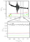Fig. 6. Torques on the star, mostly exerted by the Maxwell stresses, in the simulation b5, which is a DCE1 from Fig. 1 with the magnetospheric ejection, and mass fluxes shown in Fig. 5. The quasi-stationary interval between the vertical lines is shown in detail in the bottom panel. With the dashed (green) line is shown the torque by the stellar wind. The torques by the matter flowing onto the star through the accretion column from the distance beyond and below the corotation radius Rcor are shown with the dotted (blue) and solid (black) lines. With the dot-dashed (red) line is shown the torque exerted on the star by the magnetospheric ejection. Positive torque spins the star up, and negative slows down its rotation. In this case, the stellar rotation rate increases, so the star is spun up because of the star-disk magnetospheric interaction. In the employed units of $J_{\star }=M_{\star }{R}_{\star }^2{\mathrm{\Omega }}_{\star }$ the values correspond, in the case of YSOs, to the stellar spin-up or spin-down in Myrs.

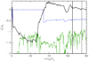Fig. 7. Torques on the star in the simulation b16 (which is the DC case), with the same strength of magnetic field, 500 G as in the simulations b5 and b8, but with a star rotating two times faster. In this case, stellar rotation will be slowed down by the torque, because more of the torque comes from the disk beyond the corotation radius Rcor. The meanings behind the lines are the same as in the previous figure.

A case when a stellar rotation is being slowed down is shown in Fig. 7. Stellar magnetic field in this case is of the same strength as in the previous example, but the star is rotating faster, and it turns out that more of the torque on the stellar surface comes from the region in the disk beyond the corotation radius.

5. Trends in torques acting on a star

We go on to analyze the results from our simulations to find trends in the solutions with different parameters. The torques are computed in the cases with varying strengths of the stellar magnetic field, stellar rotation rates, and disk resistivities. To illustrate the trends, we plot in Figs. 8–12 the functions with different coefficients, using triangles, circles and squares, while approximately following the lines obtained from simulations. If one function does not match all the cases, the lines indicate different functions.

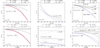Fig. 8. Components of the torque (expressed in units of J⋆) exerted on the star in the cases a,b,c,d(1,5,9,13), with αm = 0.1, when a magnetospheric ejection is launched from the star-disk magnetosphere. With the square, circle and triangle symbols are plotted approximate matching functions, indicated in each panel. Positive torque speeds the star up, negative slows it down. Top panels: Trends in torque components for cases with different stellar magnetic field strengths, as a function of the stellar rotation rate. Bottom panels: Same results as in the top panels, but given as a function of stellar magnetic field strength, organized by the different stellar rotation rates. Red lines in the left panels mark the examples of fitted lines (see text).

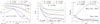Fig. 9. Torques by the stellar wind, ${\dot{J}}_{\mathrm{SW}}$ (expressed in units of J⋆) in terms of the dependence of the stellar rotation rate in the cases with the magnetospheric ejection, αm = 0.1, (left). In all the cases except for the slowest stellar rotation rates, ${\dot{J}}_{\mathrm{SW}}/J_{\star }$ drops with ${\mathrm{\Omega }}_{\star }^3$ dependence. ${\dot{J}}_{\mathrm{SW}}/J_{\star }$ is increasingly negative with the increase in stellar magnetic field strength and rotation rate, and is also decreasing slightly with 1/αm (middle). Mass fluxes in the stellar wind in the cases with the fastest stellar rotation rates in our simulations (right) also mostly decrease slightly with 1/αm. The y-label multiplication factor is given in the left upper corner of this panel.

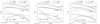Fig. 10. Torques by the stellar wind ${\dot{J}}_{\mathrm{SW}}$ (expressed in units of J⋆) in dependence of the stellar rotation rate in the cases without magnetospheric ejection (αm = 0.4, 0.7, 1.0). With the square, circle and triangle symbols are plotted approximate matching functions, indicated in each panel. In most of the cases, ${\dot{J}}_{\mathrm{SW}}$ is increasingly negative with the increase in stellar magnetic field strength and rotation rate. The cases with slower stellar rotation often do not match the approximated functions.

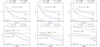Fig. 11. Torques, ${\dot{J}}_{\star }$, (expressed in units of J⋆) exerted on the star by material infalling from the disk in all the cases without magnetospheric ejection: these are all the cases except a,b,c,d(1,5,9,13), with the resistive coefficient αm = 0.4, 0.7 and 1.0. Approximate matching functions and trends in solutions with different stellar rotation rates and magnetic field strengths are shown as ${\dot{J}}_{\star }({\mathrm{\Omega }}_{\star })/J_{\star }$ (top) and ${\dot{J}}_{\star }(B_{\star })/J_{\star }$ (bottom). The dependence on αm is small.

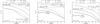Fig. 12. Total torques in the system ${\dot{J}}_{\mathrm{tot}}(B_{\star })$, (expressed in units of J⋆) in the cases without magnetospheric ejection from Fig. 11 all but a,b,c,d(1,5,9,13). Results with the same resistive coefficient, αm, are shown together and corresponding matching functions are outlined. The dependence on αm is small.

As an example, the goodness of fit shown in the top leftmost panel in the solutions with α_m = 0.1 in Fig. 8, measured by the R-squared, is 0.906 and 0.960 for ${\dot{J}}_{\mathrm{out}}({\mathrm{\Omega }}_{\star })/J_{\star }$ expressed as $-130{\mathrm{\Omega }}_{\star }^3$ and $-130{\mathrm{\Omega }}_{\star }^3$ in the cases with Ω_⋆/Ω_br equal to 0.15 and 0.20, respectively. In the bottom leftmost panel, goodness of fit, measured by the R-squared is 0.930 and 0.992 for ${\dot{J}}_{\mathrm{out}}(B_{\star })/J_{\star }$ expressed as $-0.8B_{\star }^3$ and $-2.7B_{\star }^3$ in the cases with Ω_⋆/Ω_br equal to 0.15 and 0.20, respectively⁶. The magnetospheric ejection expressions here offer the best fits, for the other components the fit goodness is often less: in general, with faster rotating star and larger magnetic field in which an accretion column is not formed, the solution departs from the trend, because of the change of flow geometry in the star-disk interaction system.

A division of the solutions in sub-classes with regard to the truncation radius or disk mass accretion rate could offer better fits, as discussed in Sect. 2 of Gallet et al. (2019), to the relation to variable coefficients of proportionality in the expressions for the torques by disk accretion and magnetospheric ejections.

In the case of different mass fluxes in the various components in the flow, we computed the outcome in our simulations, which implicitly contains the information about the change in mass fluxes, as illustrated in Figs. 13 and 14 in the cases with outflow (α_m = 0.1) and with the dependence on α_m, respectively. The comparison is more reliable between the cases where the mass fluxes in the components do not vary much because of the mixing of the flows measured at the different distances and instabilities. An example of a dependence of mass flux on the parameters included in the simulation is given in the rightmost panel in Fig. 14; this pertains to the case with 0.75 kG, where the disk mass accretion rate differs for a factor of 10 between the smallest and largest values of α_m (0.1 and 1.0). The mass fluxes in other components of the flow also change.

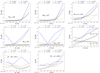Fig. 13. Mass losses in the outflow and in the stellar wind, Ṁout and ṀSW, and mass flux through the disk Ṁd in solutions with magnetospheric outflow (αm = 0.1), in terms of the dependence of the stellar rotation rate (top) and of the strength of stellar magnetic field (middle). The mass flux onto the star Ṁ⋆ is also shown (bottom). The values of Ṁout and Ṁd are computed at R = 12R⋆, while ṀSW and Ṁ⋆ are computed at the stellar surface. For illustration, shown are examples of matching functions. Note: the y-label multiplication factor is given in the left upper corner of the panels.

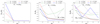Fig. 14. Components of the mass fluxes, Ṁ, in terms of the dependence of the anomalous resistive coefficient, αm, for different strengths of the stellar magnetic field in the cases with fastest stellar rotation in our simulations, Ω⋆ = 0.2Ωbr. The values of Ṁout and Ṁd are both computed at R = 12R⋆, where the flow is most stable. The latter is computed across the disk height, and corresponds to the total mass accretion rate available for distribution in the system. The component ṀSW at the same stellar rotation rate is shown together with corresponding torques in Fig. 9. Note: the y-label multiplication factor is given in the left upper corner of the panels.

As shown in Table 1, in about a third of our cases (those which have the names marked in bold letters), the total torque is positive, ${\dot{J}}_{\mathrm{tot}}>0$, meaning that the central object is spinning up. In general, the trend is that with larger stellar magnetic field and faster stellar rotation (from the top left towards the bottom right in the table), there are more spin-down cases in our simulations. Outliers from this trend, such as simulations a8, a12, c3, and d3, are often less stable cases, whereby the choice of averaging interval could influence the trend. Another possibility is that the trend is not valid for a smaller proportion of cases, for instance, because of the different mass fluxes involved for different parameters. Trends found in our simulations can be written with simple expressions, which could be compared with the results from other models, simulations, or observations, such as those in Ahuir et al. (2020), Pantolmos et al. (2020), Gallet et al. (2019).

For instance, the spin-up or spin-down timescale associated to the torques evaluated in our various simulations is on the order or Myr. If we compare this result with Gallet & Bouvier (2013), in particular, their Fig. 3, as well as the stellar rotation rates in our sample (which cover the slow and median rotating stars of their sample), we find that our results are in the correct range for solar-type young stars.

5.1. Stellar wind

The torque by stellar wind, ${\dot{J}}_{\mathrm{SW}}$, in our simulations is shown in Figs. 9 and 10. The ${\dot{J}}_{\mathrm{SW}}$ is increasingly negative with the increase in stellar rotation rate and stellar field strength. In cases with magnetospheric ejection (left), because part of the wind flow diverted into the magnetospheric ejection, the increase is lower than in the cases without the ejection (middle); it is also visible in the torques for the fastest rotating stars in our sample (right). In Fig. 15, we show the dependence of stellar wind torque on stellar magnetic field strength in the case of a viscous coefficient, α_v = 0.7, for different stellar rotation rates. With the increasing stellar rotation rate, the ${\dot{J}}_{\mathrm{SW}}/J_{\star }$ is increasingly negative, with the $B_{\star }^3$ dependence in the cases with larger magnetic fields.

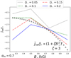Fig. 15. Torques by the stellar wind ${\dot{J}}_{\mathrm{sw}}(B_{\star })$ (expressed in units of J⋆) in cases a,b,c,d(3,7,11,15) with αm = 0.7. Triangle symbols represent approximate matching function. The torque by the stellar wind is in most of those cases increasingly negative with increasing stellar rotation rates.

The stellar wind dependence on the Alfvén radius r_A from our simulations can be compared with Eq. (10) from Gallet et al. (2019): ${\dot{J}}_{\mathrm{SW}}\propto {\mathrm{\Omega }}_{\star }{\dot{M}}_{\mathrm{SW}}{r}_{\mathrm{A}}^2$. This can be combined with their Eq. (11) for the average Alfvén radius to express:

$$\begin{array}{c}\hfill r_{\mathrm{A}}=K_1{R}_{\star }{\left(\frac{B_{\star }^2{R}_{\star }^2}{{\dot{M}}_{\mathrm{SW}}\sqrt{K_2^2{v}_{\mathrm{esc}}^2+{\mathrm{\Omega }}_{\star }^2{R}_{\star }^2}}\right)}^m,\end{array}$$(9)

which gives:

$$\begin{array}{c}\hfill \frac{\mathrm{d}{J}_{\mathrm{SW}}}{\mathrm{d}t}=-K_1^2{\mathrm{\Omega }}_{\star }{R}_{\star }^2{\dot{M}}_{\mathrm{SW}}{\left(\frac{B_{\star }^2{R}_{\star }^2}{{\dot{M}}_{\mathrm{SW}}\sqrt{K_2^2{v}_{\mathrm{esc}}^2+{\mathrm{\Omega }}_{\star }^2{R}_{\star }^2}}\right)}^{2m}.\end{array}$$(10)

Here K₁ = 1.7, K₂ = 0.0506 and m = 0.2177 are determined from numerical simulations of a stellar wind following the open field lines of a stellar dipole (Matt et al. 2012) and ${\mathit{v}}_{\mathrm{esc}}=\sqrt{2G{M}_{\star }/R_{\star }}$ is the escape velocity. The stellar magnetic field is measured at the stellar equator. In the top panels in Fig. 16, we show comparison of our results with the numbers obtained from Eq. (10) (normalized to our units of J_⋆). In the ${\dot{J}}_{\mathrm{SW}}$ cases (shown in the middle panels), we obtained in the simulations the same direction of the trend gradient as predicted, and our results are in agreement with the prediction within an order of magnitude⁷. The constant factor of 3 to 5 between their results and our simulations can easily be overcome by taking into account the change in factor K₁ and adjusting the different mass fluxes, as these authors predicted. In the results shown in the middle bottom panel in the same figure, we multiply K₁ by 2.35 to obtain a much better agreement.

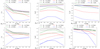Fig. 16. Comparison of our results (shown in solid lines) with the results from Gallet et al. (2019; shown in dashed lines) expressed in our units of J⋆ (top). The line colors correspond to the same magnetic field strengths in both solid and dashed lines. In the leftmost panel, Kacc = 1 was set in Eq. (12), and K1 = 1.7 and K2 = 0.0506, m = 0.2177 in Eqs. (9) and (10). The results from our simulations differ from Gallet et al. (2019) predictions, in which they assumed those factors to be constant. In our simulations, those quantities are self-consistently adjusting. Examples of curves (bottom) for the same models by Gallet et al. (2019) as in the top panels (shown with the dashed lines) with the accretion factors Kacc, KME, and K1 modified in such a way to (at least in some of the solutions) better match the results from our simulations, shown with the solid lines. The text gives details on the modifications.

The relations for ${\dot{J}}_{\mathrm{SW}}$ reported in Gallet & Bouvier (2013) and Gallet et al. (2019) have been confirmed by observations (Gallet & Bouvier 2015).

5.2. Cases with magnetospheric ejection

Flows and associated magnetic configurations in star-disk system are the most complicated in the cases with α_m = 0.1, when a magnetospheric ejection is launched from the magnetosphere. It carries away part of the material from the magnetosphere, together with its angular momentum.

The torques exerted on the star by a magnetospheric interaction with such ejection, ${\dot{J}}_{\mathrm{out}}$, and by the material infalling from the disk onto the star, ${\dot{J}}_{\star }$, are shown in Fig. 8, together with total torques in the system. The same results are shown in relations to different quantities, to reveal trends in the solutions.

We find that torque on the star exerted by the magnetospheric ejection, which slows down the star, increases with the fourth power of rotation rate, as shown in the left top and bottom panels in Fig. 8 (taking into account the J_⋆ ∝ Ω_⋆ dependence from Sect. 4): ${\dot{J}}_{\mathrm{out}}({\mathrm{\Omega }}_{\star })\propto (-{\mathrm{\Omega }}_{\star }^4)$, and with ${\dot{J}}_{\mathrm{out}}({\mathrm{\Omega }}_{\star },B_{\star })\propto (-{\mathrm{\Omega }}_{\star }{B}_{\star }^3)$. The goodness of such fits is high (R² = 0.992) for the larger rotation rates and stellar magnetic fields, for instance, the more exact least-squares fits to the polynomial $a_1{B}_{\star }^3+a_2{B}_{\star }^2+a_3{B}_{\star }+a_4$ would give only a slightly better fit of the order R² = 0.992. For weaker magnetic fields of 0.25 and 0.5 kG and more slowly rotating stars with 0.05 and 0.1 Ω_⋆/Ω_br, the dependences on the stellar rotation rates and stellar magnetic field are weak and rather linear.

The trend in ${\dot{J}}_{\mathrm{out}}$ is increasing in both cases: with the larger magnetic field and faster stellar rotation, the negative torque on a star is increasing and the star is slowing down faster. The matter load in the magnetospheric ejection is typically two to four orders of magnitude smaller than the inflow onto the star. In the case of YSOs, it yields values in the range of 10⁻¹¹ − 10⁻¹³ M_⊙ yr⁻¹.

Torques exerted on a star by material in-falling onto it through the accretion column are shown in the middle panels in Fig. 8. With the different field strengths, shown in the top middle panel, the torque does not change the stellar rotation rate: ${\dot{J}}_{\star }/J_{\star }\propto 1/{\mathrm{\Omega }}_{\star }\Rightarrow {\dot{J}}_{\star }=\mathrm{const}$. In the bottom middle panel, where the same results are organized by the different stellar rotation rates, we note only a weak dependence on the ${\mathrm{\Omega }}_{\star }{B}_{\star }^3$. The results in this panel can be related to the stellar field to match the results for other resistivities from Fig. 11. The obtained proportionality to ${\mathrm{\Omega }}_{\star }{B}_{\star }^3$ gives a good agreement for the faster rotating stars, while for more slowly rotating stars, the dependence is not compelling. Still, there is a clear trend in decrease of ${\dot{J}}_{\star }$ with faster stellar rotation: a faster rotating star is less slowed down by the infalling material⁸. With the larger magnetic field and faster rotation, the mass load in the outflow is larger, as shown in Fig. 13. A larger centrifugal force, because of the larger mass in the outflow, would exert a larger torque. This could contribute to the ${\dot{J}}_{\mathrm{out}}\propto {\mathrm{\Omega }}_{\star }^4$ dependence.

We compare our result with Gallet et al. (2019), adopting their Eq. (9):

$$\begin{array}{c}\hfill \frac{\mathrm{d}{J}_{\mathrm{out}}}{\mathrm{d}t}=K_{\mathrm{ME}}\frac{B_{\mathrm{dip}}^2{R}_{\star }^6}{R_{\mathrm{t}}^3}[K_{\mathrm{rot}}-{\left(\frac{R_{\mathrm{t}}}{R_{\mathrm{cor}}}\right)}^{3/2}].\end{array}$$(11)

Our results (shown in the right top panel in Fig. 16), do not match their prediction well for the larger stellar fields. For smaller magnetic field strengths and stellar rotation rates, the match is improved. The difference stems from the constants K_ME and K_rot, which would change with mass accretion rate and the ratio of truncation and corotation radius (see the discussion in Sect. 2.3.4 in Gallet et al. 2019). We show, in the bottom right panel in the same Fig. 16, the result with changed K_ME and K_rot (multiplied with factors 0.05 and 2.1, respectively), which improves the outcome, for instance, in the case of Ω_⋆/Ω_br = 0.15. Similar tuning could be done in each of the cases, but this is not our task here: in our simulations, the mass fluxes and radii are matching self-consistently, including the varying mass fluxes in different parts of the flow (as shown in Fig. 14).

The total torque in the system ${\dot{J}}_{\mathrm{tot}}/J_{\star }$, with α_m = 0.1, is shown in the rightmost panels in Fig. 8. It is following the same proportionality to $B_{\star }^3$ and ${\mathrm{\Omega }}_{\star }^3$. Since J_⋆ ∝ Ω_⋆, we have ${\dot{J}}_{\mathrm{tot}}\propto {\mathrm{\Omega }}_{\star }{B}_{\star }^3$ and ${\dot{J}}_{\mathrm{tot}}\propto {\mathrm{\Omega }}_{\star }^4$.

From the amounts of torque in the components, we see that magnetospheric ejection dominates in the net torque of the system. The critical value of stellar rotation rate at which the switch from a spin-up to a spin-down occurs is about Ω_⋆ = 0.1Ω_br.

5.3. Cases without magnetospheric ejection

Our results with a resistive coefficient of α_m > 0.1 do not show any magnetospheric ejection, resulting in a simpler flow pattern and field configuration (shown in the top panel in Fig. 1).

Torques exerted on a star by infalling material from the disk through an accretion column are shown in Fig. 11. The dependence on the stellar rotation rate normalized to J_⋆ is, again, ${\dot{J}}_{\star }({\mathrm{\Omega }}_{\star })=\mathrm{const}$ and on the magnetic field, it is ${\dot{J}}_{\star }(B_{\star })\propto B_{\star }^3$; here, it is also ${\dot{J}}_{\star }({\mathrm{\Omega }}_{\star },B_{\star })\propto {\mathrm{\Omega }}_{\star }{B}_{\star }^3$.

We checked that similar trends are followed by ${\dot{J}}_{R<R_{\mathrm{cor}}}$, which is the leading term in the sum making the ${\dot{J}}_{\star }$. The contribution from ${\dot{J}}_{R>R_{\mathrm{cor}}}$ is in most cases an order of magnitude smaller than ${\dot{J}}_{R<R_{\mathrm{cor}}}$.

We again compare our results with the Gallet et al. (2019) estimate. The torque exerted on the star by the material inflowing through the accretion column can be estimated by Eqs. (4)–(5) from Gallet et al. (2019; ${\dot{J}}_{\mathrm{acc}}$ in their notation):

$$\begin{array}{c}\hfill {\dot{J}}_{\mathrm{acc}}=\frac{\mathrm{d}{J}_{\star }}{\mathrm{d}t}=K_{\mathrm{acc}}{\dot{M}}_{\mathrm{acc}}\sqrt{GM{R}_{\mathrm{t}}},\end{array}$$(12)

with

$$\begin{array}{c}\hfill R_{\mathrm{t}}=K_{\mathrm{t}}{\left(\frac{B_{\mathrm{dip}}^4{R}_{\star }^{12}}{G{M}_{\star }{\dot{M}}_{\mathrm{acc}}^2}\right)}^{1/7},\end{array}$$(13)

from Bessolaz et al. (2008) and with K_acc = 1 for the cases without magnetospheric ejections. The comparison with the results in our simulations is shown in Fig. 16. Our values match their prediction only at some values; however, for many, the discrepancy between the results from our simulations and their prediction is larger, and the action of torque is also different. Instead of speeding the star up, in our simulations, it is slowing it down.

In the bottom left panel of Fig. 16, we show the same results from our simulations, but with the computation of torques (shown with dashed lines) performed by multiplying the factors K_acc with 1.1, 0.4, −0.5, and −2.5, respectively, for the increasing stellar field strengths, to better match the results from our simulations. This would amount to changes in the mass accretion rate with different field strengths. Again, in our simulations, this is done self-consistently.

All the components shown above contribute to the total torque exerted on the star, shown in Fig. 12 for the α_m = 0.4, 0.7 and 1 (left to right panels, respectively). It is the sum of components from the different parts of flow and field configurations in the system.

In the cases with fastest stellar rotation in our study, Ω_⋆ = 0.2, the total torque in the system is slightly out of the trend. We present such cases in Fig. 17, also adding the cases with α_m = 0.1, to show that they follow a trend with the increasing magnetic field strengths. In the cases with slower stellar rotation or smaller stellar field, the total torque is often positive and its variation less steep. Another result that can be appreciated from this figure (and this is another reason why we added also the α_m = 0.1 cases) is that the total torque ${\dot{J}}_{\mathrm{tot}}$ does not depend much on the resistive coefficient, α_m. The reason for departing from the trend in the cases with faster stellar rotation is not the resistivity in the disk, but the different geometry of the system: the disk is pushed away from the star and there is no accretion column. Most of the torque on the star now comes from the part of the system beyond the corotation radius, R_cor, slowing the star down. In the bottom panel in the same figure we show the dependence of total torque on the stellar rotation rates with α_m for the simulations with B_⋆ = 0.5 kG. Here, we also see weak dependence on α_m.

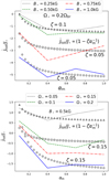Fig. 17. Total torques in the system ${\dot{J}}_{\mathrm{tot}}({\alpha }_{\mathrm{m}})$ (expressed in units of J⋆) in cases a,b,c,d(13,14,15,16), with fastest stellar rotation in our sample, Ω⋆ = 0.2 (top) and in cases b(1–16) with B⋆ = 0.5 kG (bottom), showing the 1/αm dependence. Similar results are obtained in most of the other cases.

In Fig. 18, we show the dependence of total torque in the system (normalized to the J_⋆) with the stellar rotation rate, Ω_⋆, and its trend with the magnetic field, B_⋆, in cases with α_m = 1. When we include the J_⋆ ∝ Ω_⋆ dependence, we find that ${\dot{J}}_{\mathrm{tot}}({\mathrm{\Omega }}_{\star })=\mathrm{const}$. Similar results are obtained with smaller α_m, namely, in most of the cases, we obtain a spin-down for the central object. Here, we also see that the critical stellar rotation rate for a switch from spin-up to spin-down is between 0.07 and 0.11 Ω_br, as in the cases with magnetospheric ejection.

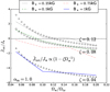Fig. 18. Total torques (expressed in units of J⋆) for the anomalous resistivity coefficient αm = 1.0 in the cases a,b,c,d(4,8,12,16) with different B⋆, in terms of the dependence of stellar rotation rate, ${\dot{J}}_{\mathrm{tot}}({\mathrm{\Omega }}_{\star })$. The total torque in the system is increasingly negative with the increase in stellar field, B⋆.

In most of the cases without magnetospheric ejection, the magnetic field is anchored in the disk beyond the corotation radius, with the accretion column positioned below the corotation radius (as in simulation b8, illustrated in Fig. 1). With the increase of stellar rotation rate, corotation radius shifts closer to the star, approaching the footpoint of the accretion column. This, in turn, can change the torque, and cause a switch between the spin-up and spin-down of the star. When the central object is slowed-down, the decrease in the stellar rotation is slower than in the cases with the magnetospheric ejection with the stronger field.

6. Conclusions

In our numerical simulations of a star-disk magnetospheric interaction, we obtained a suite of quasi-stationary solutions. We performed a parameter study based on 64 axisymmetric 2D MHD simulations, varying the disk resistivity, stellar dipole magnetic field strength, and rotation rate.

In order to assess how far the stellar magnetic field is able to connect itself into the disk, we measured the furthest anchoring radius, R_out. In our simulations, we find the following trends:

– R_out increases with the larger resistive coefficient, α_m, for all the strengths of the stellar magnetic field. This is because the field line is able to slip through the disk more easily than in less diffusive case, where it disconnects due to strong shear.

– In cases with α_m = 0.1, when a magnetospheric ejection is launched from the system, there is only a minor dependence of R_out on the stellar rotation rates for all the stellar field strengths. The increase in R_out with the stellar field strength is small in such cases. This is likely due to the field geometry and the presence of the current sheet at mid latitudes.

In all the cases, we find that the kinematic torque is negligible, implying that most of the torque comes from the magnetic interaction.

We describe the dependence of torques in the system by characterizing their magnetospheric interaction regime with approximate expressions. We obtain:

– The torque exerted on the star by a material in-falling from the disk onto the star, ${\dot{J}}_{\star }$, by a material expelled from the system in a magnetospheric ejection, ${\dot{J}}_{\mathrm{out}}$, and a total torque in the system, ${\dot{J}}_{\mathrm{tot}}$, we can write in all the cases as:

$$\begin{array}{c}\hfill {\dot{J}}_{\star },{\dot{J}}_{\mathrm{out}},{\dot{J}}_{\mathrm{tot}}\propto {\mathrm{\Omega }}_{\star }{B}_{\star }^3.\end{array}$$

– In all the cases, the total torque in the system does not depend much on the resistivity coefficient, α_m.

– Our results for stellar wind are in a reasonable agreement with the theoretical and observational results on magnetospheric star-disk interaction and stellar wind from Gallet et al. (2019), with trends in ${\dot{J}}_{\mathrm{SW}}$ following the predicted expression (see Fig. 16). We show that their assumption of constant factor, K₁, is not in agreement with the results we obtained with the self-consistent treatment in MHD simulations.

– In all the cases without magnetospheric ejection, the torque exerted on the star is independent of stellar rotation rate:

$$\begin{array}{c}\hfill {\dot{J}}_{\star }({\mathrm{\Omega }}_{\star })=\mathrm{const}.\end{array}$$

In our simulations, these are all the cases with α_m > 0.1. Here, we also show that assumption of the constant, K_acc, from Gallet et al. (2019) is not in agreement with our self-consistent treatment in simulations.

– In all the cases with α_m = 0.1, abcd(1,5,9,13), a magnetospheric ejection is launched in our simulations. Most of the torque in the system in such cases is in the ejection. The component of the torque exerted on the star by such an ejection can be expressed as:

$$\begin{array}{c}\hfill {\dot{J}}_{\mathrm{out}}({\mathrm{\Omega }}_{\star })\propto {\mathrm{\Omega }}_{\star }^4.\end{array}$$

From our results we conclude that the reason for such strong dependence is the fact that the faster rotating star increases the amount of material in the outflow, which results in a larger torque and centrifugal force.

– In two-thirds of all the cases with magnetospheric ejection in our simulations, the central star is spun up. The spin-up stops in the cases with larger field and faster stellar rotation. In the cases without magnetospheric ejection, only a third are yielding a spun-up star. With the increasing stellar magnetic field or faster stellar rotation rate, we observe a switch of sign in the net torque, resulting in a spun-down star. The spin-down is also increasing with the increasing field strength or stellar rotation rate.

– The critical stellar rotation rate at which the spin-up switches to spin-down is between 0.07 and 0.11 Ω_br.

– A comparison with Gallet et al. (2019) results shows that the constant factors K_acc and K_ME from their expressions are not in agreement with the self-consistent treatment in our simulations, we instead find a variation among these prefactors. It is a consequence of changes in the mass fluxes in the different components in the flow with the different stellar rotation rates, magnetic field, and disk resistivity. For example, in our simulations, we find that in cases with magnetospheric ejections (α_m = 0.1), the mass losses through the stellar wind and outflow Ṁ_out and Ṁ_SW are both proportional to ${\Omega }_{\star }^6$ and $B_{\star }^4$, and the mass fluxes ${\dot{M}}_{\star }$ onto the star are proportional to ${\mathrm{\Omega }}_{\star }^3$. In the cases with other α_m, scattering in the results is larger.

Here, we list the most important caveats in our work. Our sample of numerical simulations was limited to slowly⁹ rotating objects at up to 20% of the breakup velocity at the equator. For the faster rotating objects, an axial outflow often forms, which would further complicate the description. We started a separate line of study for such cases (Kotek et al. 2020), where a more thorough study of torque in magnetospheric ejections will, in connection with the axial outflow, be more complete. Mass fluxes in the different components of the flow demand a separate study, probably with an additional division of the results with a positioning of the characteristic radii in the system. Also, we refer here only to stellar dipole fields, when it is known that multipole stellar fields are closer to reality-this is another separate line in our research (Cieciuch & Čemelji 2022). Another complication we avoided by setting the viscous anomalous coefficient α_v = 1 in all simulations to avoid backflow in the disk. Such an outflow near the disk midplane, directed away from the star was also found in numerical computations with alpha-viscosity (Kley & Lin 1992; Igumenshchev et al. 1996; Rozyczka et al. 1994) and with the magneto-rotational instability (White et al. 2020; Mishra et al. 2020a). We describe it elsewhere (Mishra et al. 2020b,c, 2023). In our computation of torques, we checked that the field in most of the disk is at least one order of magnitude smaller than the stellar field, so we neglected the effect of magnetic field inside the accretion disk on the result. However, Naso et al. (2013) showed that in some cases the disk field affects the torque on the star; in our solutions, it would be in the cases when corotation radius is nearby the footpoint of the accretion column. We leave this point for a future study.

Acknowledgments

M.Č. acknowledges the Czech Science Foundation (GAČR) grant No. 21-06825X and the Polish NCN grant 2019/33/B/STA9/01564. M.Č. developed the setup for star-disk simulations while in CEA, Saclay, under the ANR Toupies grant, and a collaboration with the Croatian STARDUST project through HRZZ grant IP-2014-09-8656 is acknowledged. M.Č. thanks to the support by the International Space Science Institute (ISSI) in Bern, which hosted the International Team project #495 (Feeding the spinning top) with its inspiring discussions. A.S. Brun acknowledges support by CNES PLATO grant and ERC Stars 2. We thank IDRIS (Turing cluster) in Orsay, France, ASIAA (PL and XL clusters) in Taipei, Taiwan and NCAC (PSK and CHUCK clusters) in Warsaw, Poland, for access to Linux computer clusters used for the high-performance computations. The PLUTO team, in particular A. Mignone, is thanked for the possibility to use the code.

References

All Tables

All Figures

Fig. 1. Four typical geometries in our solutions: Disk+Column (DC), Disk (D), Disk+Column+Ejection1 (DCE1), and Disk+Column+Ejection2 (DCE2) illustrated by snapshots in quasi-stationary states in simulations b8, d12, b5, and c9 (top to bottom, respectively). We show the density in a logarithmic color grading, with a sample of magnetic field lines in red solid lines. White lines labeled a, a’, b, and c delimit the components of the flow between which we integrate the fluxes; Rin, Rout and Rcor are the inner disk edge, the furthest outer reach of closed stellar field in the disk and the corotation radius, respectively.

In the text

Fig. 2. Positions of the anchoring radius, Rout, for the furthest stellar magnetic field line in the disk that still reaches the star and the inner disk radius, Rin. Top panels: Rout increases with the increasing resistive coefficient αm for all stellar magnetic fields (left) and position of the Rout as a function of stellar rotation rate in the cases without magnetospheric ejection shows a decreasing trend with the stellar magnetic field (right). It is only in the cases with B⋆ = 0.5 kG that we obtain a departure from this trend, with the largest Rout at the slowest stellar rotation rate. Bottom panels: Inner disk radius, Rin, is increasing in the majority of the cases with same parameters as in the above panels for Rout.

In the text

Fig. 3. Variation of the furthest anchoring radius of the stellar field in the disk Rout with the stellar field in the cases with αm = 0.1 (which are all with a magnetospheric ejection launched from the system) is not large (left). Without the magnetospheric ejection, the scattering in this result is much larger. Inner disk radius Rin in the same cases displays a clear increasing trend with the increase of stellar magnetic field (right).

In the text

Fig. 4. Toroidal magnetic field values along the disk surface (top) and along the disk height (measured from the disk equatorial plane) at R = 12R⋆ (bottom) are shown in terms of their dependence of stellar rotation rates. The values are averaged over 10 stellar rotation periods during the quasi-stationary states, in the cases with αm = 1 and B⋆ = 500 G (simulations b1, b5, b9, and b13). In black, green, blue, and red dashed lines we display the values for 0.05, 0.1, 0.15, and 0.2 of Ωbr, respectively. The black solid lines provide the reference for typical radial and vertical dependence.

In the text

Fig. 5. Mass fluxes in the code units ${\dot{M}}_0={\rho }_{\mathrm{d}0}\sqrt{G{M}_{\star }{R}_{\star }^3}$ in the various flow components in the simulation b5, shown in Fig. 1. With vertical solid lines is indicated the time interval in which we average the fluxes in each of the flow components. With the solid (black) line is shown the mass flux through the disk at R = 12R⋆ and with the dotted (blue) line the mass flux loaded onto the star through the accretion column. Those two fluxes are much larger than the fluxes in the other components of the flow. The mass flux flowing through the magnetospheric ejection at the radius R = 12R⋆ is shown with the dot-dashed (red) line, and the mass flux into the stellar wind from the vicinity of the stellar surface is shown with the long-dashed (green) line.

In the text

Fig. 6. Torques on the star, mostly exerted by the Maxwell stresses, in the simulation b5, which is a DCE1 from Fig. 1 with the magnetospheric ejection, and mass fluxes shown in Fig. 5. The quasi-stationary interval between the vertical lines is shown in detail in the bottom panel. With the dashed (green) line is shown the torque by the stellar wind. The torques by the matter flowing onto the star through the accretion column from the distance beyond and below the corotation radius Rcor are shown with the dotted (blue) and solid (black) lines. With the dot-dashed (red) line is shown the torque exerted on the star by the magnetospheric ejection. Positive torque spins the star up, and negative slows down its rotation. In this case, the stellar rotation rate increases, so the star is spun up because of the star-disk magnetospheric interaction. In the employed units of $J_{\star }=M_{\star }{R}_{\star }^2{\mathrm{\Omega }}_{\star }$ the values correspond, in the case of YSOs, to the stellar spin-up or spin-down in Myrs.

In the text

Fig. 7. Torques on the star in the simulation b16 (which is the DC case), with the same strength of magnetic field, 500 G as in the simulations b5 and b8, but with a star rotating two times faster. In this case, stellar rotation will be slowed down by the torque, because more of the torque comes from the disk beyond the corotation radius Rcor. The meanings behind the lines are the same as in the previous figure.

In the text

Fig. 8. Components of the torque (expressed in units of J⋆) exerted on the star in the cases a,b,c,d(1,5,9,13), with αm = 0.1, when a magnetospheric ejection is launched from the star-disk magnetosphere. With the square, circle and triangle symbols are plotted approximate matching functions, indicated in each panel. Positive torque speeds the star up, negative slows it down. Top panels: Trends in torque components for cases with different stellar magnetic field strengths, as a function of the stellar rotation rate. Bottom panels: Same results as in the top panels, but given as a function of stellar magnetic field strength, organized by the different stellar rotation rates. Red lines in the left panels mark the examples of fitted lines (see text).

In the text

Fig. 9. Torques by the stellar wind, ${\dot{J}}_{\mathrm{SW}}$ (expressed in units of J⋆) in terms of the dependence of the stellar rotation rate in the cases with the magnetospheric ejection, αm = 0.1, (left). In all the cases except for the slowest stellar rotation rates, ${\dot{J}}_{\mathrm{SW}}/J_{\star }$ drops with ${\mathrm{\Omega }}_{\star }^3$ dependence. ${\dot{J}}_{\mathrm{SW}}/J_{\star }$ is increasingly negative with the increase in stellar magnetic field strength and rotation rate, and is also decreasing slightly with 1/αm (middle). Mass fluxes in the stellar wind in the cases with the fastest stellar rotation rates in our simulations (right) also mostly decrease slightly with 1/αm. The y-label multiplication factor is given in the left upper corner of this panel.

In the text

Fig. 10. Torques by the stellar wind ${\dot{J}}_{\mathrm{SW}}$ (expressed in units of J⋆) in dependence of the stellar rotation rate in the cases without magnetospheric ejection (αm = 0.4, 0.7, 1.0). With the square, circle and triangle symbols are plotted approximate matching functions, indicated in each panel. In most of the cases, ${\dot{J}}_{\mathrm{SW}}$ is increasingly negative with the increase in stellar magnetic field strength and rotation rate. The cases with slower stellar rotation often do not match the approximated functions.

In the text

Fig. 11. Torques, ${\dot{J}}_{\star }$, (expressed in units of J⋆) exerted on the star by material infalling from the disk in all the cases without magnetospheric ejection: these are all the cases except a,b,c,d(1,5,9,13), with the resistive coefficient αm = 0.4, 0.7 and 1.0. Approximate matching functions and trends in solutions with different stellar rotation rates and magnetic field strengths are shown as ${\dot{J}}_{\star }({\mathrm{\Omega }}_{\star })/J_{\star }$ (top) and ${\dot{J}}_{\star }(B_{\star })/J_{\star }$ (bottom). The dependence on αm is small.

In the text

	Fig. 12. Total torques in the system ${\dot{J}}_{\mathrm{tot}}(B_{\star })$, (expressed in units of J⋆) in the cases without magnetospheric ejection from Fig. 11 all but a,b,c,d(1,5,9,13). Results with the same resistive coefficient, αm, are shown together and corresponding matching functions are outlined. The dependence on αm is small.
In the text

Fig. 13. Mass losses in the outflow and in the stellar wind, Ṁout and ṀSW, and mass flux through the disk Ṁd in solutions with magnetospheric outflow (αm = 0.1), in terms of the dependence of the stellar rotation rate (top) and of the strength of stellar magnetic field (middle). The mass flux onto the star Ṁ⋆ is also shown (bottom). The values of Ṁout and Ṁd are computed at R = 12R⋆, while ṀSW and Ṁ⋆ are computed at the stellar surface. For illustration, shown are examples of matching functions. Note: the y-label multiplication factor is given in the left upper corner of the panels.

In the text

Fig. 14. Components of the mass fluxes, Ṁ, in terms of the dependence of the anomalous resistive coefficient, αm, for different strengths of the stellar magnetic field in the cases with fastest stellar rotation in our simulations, Ω⋆ = 0.2Ωbr. The values of Ṁout and Ṁd are both computed at R = 12R⋆, where the flow is most stable. The latter is computed across the disk height, and corresponds to the total mass accretion rate available for distribution in the system. The component ṀSW at the same stellar rotation rate is shown together with corresponding torques in Fig. 9. Note: the y-label multiplication factor is given in the left upper corner of the panels.

In the text

	Fig. 15. Torques by the stellar wind ${\dot{J}}_{\mathrm{sw}}(B_{\star })$ (expressed in units of J⋆) in cases a,b,c,d(3,7,11,15) with αm = 0.7. Triangle symbols represent approximate matching function. The torque by the stellar wind is in most of those cases increasingly negative with increasing stellar rotation rates.
In the text

Fig. 16. Comparison of our results (shown in solid lines) with the results from Gallet et al. (2019; shown in dashed lines) expressed in our units of J⋆ (top). The line colors correspond to the same magnetic field strengths in both solid and dashed lines. In the leftmost panel, Kacc = 1 was set in Eq. (12), and K1 = 1.7 and K2 = 0.0506, m = 0.2177 in Eqs. (9) and (10). The results from our simulations differ from Gallet et al. (2019) predictions, in which they assumed those factors to be constant. In our simulations, those quantities are self-consistently adjusting. Examples of curves (bottom) for the same models by Gallet et al. (2019) as in the top panels (shown with the dashed lines) with the accretion factors Kacc, KME, and K1 modified in such a way to (at least in some of the solutions) better match the results from our simulations, shown with the solid lines. The text gives details on the modifications.

In the text

	Fig. 17. Total torques in the system ${\dot{J}}_{\mathrm{tot}}({\alpha }_{\mathrm{m}})$ (expressed in units of J⋆) in cases a,b,c,d(13,14,15,16), with fastest stellar rotation in our sample, Ω⋆ = 0.2 (top) and in cases b(1–16) with B⋆ = 0.5 kG (bottom), showing the 1/αm dependence. Similar results are obtained in most of the other cases.
In the text

	Fig. 18. Total torques (expressed in units of J⋆) for the anomalous resistivity coefficient αm = 1.0 in the cases a,b,c,d(4,8,12,16) with different B⋆, in terms of the dependence of stellar rotation rate, ${\dot{J}}_{\mathrm{tot}}({\mathrm{\Omega }}_{\star })$. The total torque in the system is increasingly negative with the increase in stellar field, B⋆.
In the text

References

- Ahuir, J., Brun, A. S., & Strugarek, A. 2020, A&A, 635, A170 [NASA ADS] [CrossRef] [EDP Sciences] [Google Scholar]
- Bessolaz, N., Zanni, C., Ferreira, J., Keppens, R., & Bouvier, J. 2008, A&A, 478, 155 [NASA ADS] [CrossRef] [EDP Sciences] [Google Scholar]
- Bouvier, J., & Cébron, D. 2015, MNRAS, 453, 3720 [Google Scholar]
- Cieciuch, F., & Čemeljić, M. 2022, XL Polish Astronomical Society Meeting, eds. E. Szuszkiewicz, A. Majczyna, K. Małek, et al., 12, 192 [Google Scholar]
- Čemeljić, M. 2019, A&A, 624, A31 [NASA ADS] [CrossRef] [EDP Sciences] [Google Scholar]
- Čemeljić, M., Parthasarathy, V., & Kluźniak, W. 2017, J. Phys. Conf. Ser., 932, 012028 [CrossRef] [Google Scholar]
- Čemeljić, M., Kluźniak, W., & Parthasarathy, V. 2019, ArXiv e-prints [arXiv:1907.12592] [Google Scholar]
- Gallet, F., & Bouvier, J. 2013, A&A, 556, A36 [NASA ADS] [CrossRef] [EDP Sciences] [Google Scholar]
- Gallet, F., & Bouvier, J. 2015, A&A, 577, A98 [NASA ADS] [CrossRef] [EDP Sciences] [Google Scholar]
- Gallet, F., Zanni, C., & Amard, L. 2019, A&A, 632, A6 [NASA ADS] [CrossRef] [EDP Sciences] [Google Scholar]
- Ghosh, P., & Lamb, F. K. 1979a, ApJ, 232, 259 [Google Scholar]
- Ghosh, P., & Lamb, F. K. 1979b, ApJ, 234, 296 [Google Scholar]
- Igumenshchev, I. V., Chen, X., & Abramowicz, M. A. 1996, MNRAS, 278, 236 [NASA ADS] [CrossRef] [Google Scholar]
- Illarionov, A. F., & Sunyaev, R. A. 1975, A&A, 39, 185 [NASA ADS] [Google Scholar]
- Kley, W., & Lin, D. N. C. 1992, ApJ, 397, 600 [CrossRef] [Google Scholar]
- Kluzniak, W., & Kita, D. 2000, ArXiv e-prints [arXiv:astro-ph/0006266] [Google Scholar]
- Kotek, A., Čemeljić, M., Kluźniak, W., Bollimpalli, D. A., et al. 2020, in XXXIX Polish Astronomical Society Meeting, eds. K. Małek, M. Polińska, A. Majczyna, et al., 10, 275 [NASA ADS] [Google Scholar]
- Lovelace, R. V. E., Romanova, M. M., & Bisnovatyi-Kogan, G. S. 1999, ApJ, 514, 368 [Google Scholar]
- Matt, S., & Pudritz, R. E. 2005, ApJ, 632, L135 [Google Scholar]
- Matt, S. P., MacGregor, K. B., Pinsonneault, M. H., & Greene, T. P. 2012, ApJ, 754, L26 [Google Scholar]
- Mignone, A., Bodo, G., Massaglia, S., et al. 2007, ApJS, 170, 228 [Google Scholar]
- Mishra, B., Begelman, M. C., Armitage, P. J., & Simon, J. B. 2020a, MNRAS, 492, 1855 [NASA ADS] [CrossRef] [Google Scholar]
- Mishra, R., Čemeljić, M., Kluźniak, W., et al. 2020b, in XXXIX Polish Astronomical Society Meeting, eds. K. Małek, M. Polińska, A. Majczyna, et al., 10, 147 [NASA ADS] [Google Scholar]
- Mishra, R., Čemeljić, M., & Kluźniak, W. 2020c, ArXiv e-prints [arXiv:2012.13194] [Google Scholar]
- Mishra, R., Čemeljić, M., & Kluźniak, W. 2023, MNRAS, 523, 4708 [NASA ADS] [CrossRef] [Google Scholar]
- Naso, L., Kluźniak, W., & Miller, J. C. 2013, MNRAS, 435, 2633 [CrossRef] [Google Scholar]
- Pantolmos, G., Zanni, C., & Bouvier, J. 2020, A&A, 643, A129 [NASA ADS] [CrossRef] [EDP Sciences] [Google Scholar]
- Romanova, M. M., Ustyugova, G. V., Koldoba, A. V., & Lovelace, R. V. E. 2009, MNRAS, 399, 1802 [Google Scholar]
- Romanova, M. M., Ustyugova, G. V., Koldoba, A. V., & Lovelace, R. V. E. 2013, MNRAS, 430, 699 [Google Scholar]
- Rozyczka, M., Bodenheimer, P., & Bell, K. R. 1994, ApJ, 423, 736 [NASA ADS] [CrossRef] [Google Scholar]
- White, C. J., Quataert, E., & Gammie, C. F. 2020, ApJ, 891, 63 [NASA ADS] [CrossRef] [Google Scholar]
- Zanni, C., & Ferreira, J. 2009, A&A, 508, 1117 [CrossRef] [EDP Sciences] [Google Scholar]
- Zanni, C., & Ferreira, J. 2013, A&A, 550, A99 [NASA ADS] [CrossRef] [EDP Sciences] [Google Scholar]
All Tables
64 star-disk magnetospheric interaction simulations in a setup detailed in Čemeljić (2019).