| Issue |
A&A
Volume 678, October 2023
|
|
|---|---|---|
| Article Number | A57 | |
| Number of page(s) | 16 | |
| Section | Astrophysical processes | |
| DOI | https://doi.org/10.1051/0004-6361/202140637 | |
| Published online | 04 October 2023 | |
Magnetically threaded accretion disks in resistive magnetohydrodynamic simulations and asymptotic expansion
1
Research Centre for Computational Physics and Data Processing, Institute of Physics, Silesian University in Opava, Bezručovo nám. 13, 746 01 Opava, Czech Republic
2
Nicolaus Copernicus Astronomical Center, Polish Academy of Sciences, Bartycka 18, 00-716 Warsaw, Poland
e-mail: This email address is being protected from spambots. You need JavaScript enabled to view it.
3
Academia Sinica, Institute of Astronomy and Astrophysics, PO Box 23-141 Taipei 106, Taiwan
4
Höchstleistungsrechenzentrum Stuttgart, Nobelstraße 19, 70569 Stuttgart, Germany
Received:
22
February
2021
Accepted:
16
August
2023
Abstract
Aims. A realistic model of magnetic linkage between a central object and its accretion disk is a prerequisite for understanding the spin history of stars and stellar remnants. To this end, we aim to provide an analytic model in agreement with magnetohydrodynamic (MHD) simulations.
Methods. For the first time, we wrote a full set of stationary asymptotic expansion equations of a thin magnetic accretion disk, including the induction and energy equations. We also performed a resistive MHD simulation of an accretion disk around a star endowed with a magnetic dipole, using the publicly available code PLUTO. We compared the analytical results with the numerical solutions, and discussed the results in the context of previous solutions of the induction equation describing the star-disk magnetospheric interaction.
Results. We found that the magnetic field threading the disk is suppressed by orders of magnitude inside thin disks, so the presence of the stellar magnetic field does not strongly affect the velocity field, nor the density profile inside the disk. Density and velocity fields found in the MHD simulations match the radial and vertical profiles of the analytic solution. Qualitatively, the MHD simulations result in an internal magnetic field similar to the solutions previously obtained by solving the induction equation in the disk alone. However, the magnetic field configuration is quantitatively affected by magnetic field inflation outside the disk; this is reflected in the net torque. The torque on the star is an order of magnitude larger in the magnetic than in the non-magnetic case. Spin-up of the star occurs on a timescale comparable to the accretion timescale in the MHD case, and is an order of magnitude slower in the absence of a stellar magnetic field.
Key words: accretion / accretion disks / magnetohydrodynamics (MHD) / methods: analytical / methods: numerical / stars: neutron / X-rays: binaries
© The Authors 2023
 Open Access article, published by EDP Sciences, under the terms of the Creative Commons Attribution License (https://creativecommons.org/licenses/by/4.0), which permits unrestricted use, distribution, and reproduction in any medium, provided the original work is properly cited.
This article is published in open access under the Subscribe to Open model. This email address is being protected from spambots. You need JavaScript enabled to view it. to support open access publication.
1. Introduction
While the problem is more generally applicable to accreting stellar systems, the question of the interaction between the stellar magnetosphere and the accretion disk has gained particular prominence in discussions of spin-up and spin-down torques of X-ray pulsars. It is not controversial that the accretion disk is truncated at an inner radius where the influence of the stellar magnetosphere balances the stresses in the disk. The exact location of this inner radius, rin, depends on the model, but most expressions differ by no more than a factor of two1.
There is less agreement on the detailed disk-magnetosphere interaction and the resulting torques on the star. One school of thought assumes the disk to be perfectly conducting. Scharlemann (1978) and Aly (1980) considered the interaction of the accretion disk and the stellar magnetic field to be concentrated only in a very narrow ring near the inner edge of the disk. Simulations of the magnetosphere in the presence of a perfectly conducting disk seem to be in agreement with those ideas (Romanova et al. 2012; Parfrey et al. 2016, 2017; Parfrey & Tchekhovskoy 2016).
In another paradigm, the idealization of a perfectly conducting plasma is given up, and the stellar magnetic field is allowed to penetrate a broader region of the inner accretion disk through turbulent diffusion and reconnection (Vasyliunas 1975; Ghosh et al. 1977; Ghosh & Lamb 1979), leading to the classic picture of magnetic torques contributing to spin-up in the region rin < r < rcor and to spin-down in the region r > rcor, where  is the co-rotation radius, M⋆ is the mass of the star, and Ω⋆ its rotation rate. The resulting torques in a modified model within this paradigm were computed by Wang (1996), and the associated changes in the structure of the accretion disk by Kluźniak & Rappaport (2007); cf. Agapitou & Papaloizou (2000), Erkut & Alpar (2004). A recent paper discusses the problem in the context of ultraluminous X-ray pulsars for a modified disk solution, with the inclusion of advection (Chashkina et al. 2019). All the aforementioned analytic work assumed a thin height-integrated disk, i.e., followed the Shakura & Sunyaev (1973) scheme.
A more fundamental approach within this main-stream paradigm has been taken by Naso & Miller (2010, 2011), who actually solved the induction equation inside the accretion disk, on a fixed background of plasma variables corresponding to the Shakura & Sunyaev (1973)α-disk model. Naso et al. (2013) have performed the same task, but on the background of the Kluźniak & Kita (2000) model, computing the torque contribution from the interior of the disk (and not the disk surface alone, as was done by previous authors) and finding that different vertical zones of the disk may contribute to spin-up or spin-down regardless of whether they are inside or outside the co-rotation radius.
We would like to take the next step and to solve simultaneously and self-consistently for both the magnetic field and the fluid variables, such as the velocity field, in a magnetically threaded disk. To this end, we have developed a very stable numerical solution of an accretion disk, and have performed resistive magnetohydrodynamic (MHD) simulations of the accretion disk interacting with the stellar magnetosphere. It is numerically expensive to perform such simulations when the stellar magnetic dipole becomes too strong. For this, and other reasons it would be desirable to have arguments allowing extension of the results obtained to the more strongly magnetized regime. An analytic solution would serve this purpose admirably, but is rather hard to obtain. As a first step we will be satisfied with finding in an analytic calculation certain restrictions on the solution, as well as scaling laws which validate the MHD numerical solution, thus allowing an extension of the latter to stronger magnetic fields.
In this paper we present both our numerical resistive MHD simulation solutions to the disk-magnetosphere problem, as well as an asymptotic expansion of the governing equations which yield constraints on the magnetic field in leading orders of the dimensionless disk thickness, and allow a partial analytic solution of the problem. Our numerical simulations include the innermost part of the accretion disk and accretion column quite close to the stellar surface. While we find the formal Alfvén radius (defined as the radius at which the Alfvén and radial flow velocities become equal) to be typically about 4 stellar radii in the disk, the flow starts to lift from the disk, following the magnetic field lines to the pole, only at less than 3 stellar radii. This truncation radius of the disk also happens to be close to the co-rotation radius for our simulations. We compare our analytical solutions with the numerical ones at 6 and 15 stellar radii in the disk.
In the following, after an introduction to thin disks (Sect. 2), in Sect. 3 we present the equations that are solved in the work, and outline the results of the method of asymptotic expansion. We then present the quasi-stationary results in our numerical simulations (Sect. 4) and find the expressions for the best matches to the numerical solutions. In Sect. 5 we discuss the torques on the star, and summarize the results in Sect. 6. Appendix A contains a detailed analysis of the equations by the method of asymptotic expansion, and Appendix B contains details of the numerical setup.
2. Thin disks
Stationary disks are in vertical hydrostatic equilibrium. We restrict ourselves to geometrically thin disks with the height scale H much smaller than the radial distance r, H ≪ r, whence the radial gravitational attraction of the central body is balanced by the (differential) rotation of the disk. For such disks this rotation very closely follows the Keplerian law. It is not clear whether thin disks can extend to the direct vicinity of a (weakly magnetized) neutron star at near-Eddington accretion rates, as the inner disk would then be radiation-pressure dominated and subject to thermal instability2 on the Keplerian timescale (Shakura & Sunyaev 1976; Mishra et al. 2016; Sdowski 2016; Fragile et al. 2018). However, at lower accretion rates, or further away from the star (as in the strongly magnetized classic X-ray pulsars), the disk is gas-pressure dominated and stable. Our simulations and analytic results correspond to the gas-pressure dominated regime.
The first analytical solution for the accretion disk has been given in Shakura & Sunyaev (1973) in the α approximation, in which the stress tensor is proportional to the pressure. In that and many following works the radial solution was obtained as an average over the disk thickness, with equations in the vertical direction separately solved to obtain a hydrostatic balance. However, Urpin (1984) showed that height-averaged values of radial velocity are not representative of the disk midplane, where in fact the flow direction is directed radially outwards.
A three-dimensional, analytic solution for the velocity field and density of a steady axisymmetric, polytropic, hydrodynamical (HD) α-disk has been given in Kita (1995) and Kluźniak & Kita (2000; hereafter KK00) and confirmed in Regev & Gitelman (2002) with the use of the ideal equation of state. Equatorial backflow is present for all realistic values of the viscosity parameter (α < 0.68). These results were upheld by the results of several numerical simulations (e.g., Igumenshchev & Abramowicz 2000; Lee & Ramirez-Ruiz 2002; Mishra et al. 2020a, 2023); and also Philippov & Rafikov (2017).
As remarked in the Introduction, most of the work on the disk-magnetosphere problem was performed for Shakura & Sunyaev (1973) axially symmetric α-disks, which by their one-dimensional nature do not allow backflows. To avoid the backflow, in part for greater ease of comparison with previous work, and in part because we are considering stationary MHD solutions and we are uncertain that such solutions actually exist3 for α-disks with backflows, in this paper we assume the value α = 1 for the viscosity parameter.
We extend the KK00 solution to the case of a magnetic disk. Since the solution inside the disk depends on details of the star-disk magnetospheric interaction, we cannot solve for the magnetic field in the disk without knowing the global solution. For this reason, we perform an MHD solution of the disk initially penetrated by the dipole magnetic field of the star, and find the resulting velocity field, as well as the magnetic field configuration, which exhibits the well-known effect of field inflation. However, we will show analytically that the vertical density profile of the magnetized thin accretion disk is the same as in a hydrodynamic (HD) disk, and in the steady regime its velocity field is not affected in the leading order by the presence of the magnetic field. This is borne out by our simulations. Thus, for α = 1 the configuration of the field internal to the disk is qualitatively similar to that found by Naso & Miller (2011), who solved the induction equation on a background flow solution corresponding to the Shakura & Sunyaev (1973) solution.
An extensive set of our simulations was shown in Čemeljić (2019), where quasi-stationary solutions were obtained with various stellar rotation rates, magnetic field strengths, and magnetic Prandtl numbers. Here we focus on the case of millisecond accreting pulsars, where the disk extends very close to the stellar surface, and it is only at less than three stellar radii (r < 3R⋆) that the flow begins to follow the magnetic field lines onto the pole. For neutron stars the solution would correspond to a magnetic moment of ∼1026 G cm3 (surface field of ∼108 G). In our simulations the stellar rotation rate is at 20% of the equatorial mass-shedding limit, Ω⋆ = 0.20 Ωms.
We will confront the disk solutions from such simulations with the requirements obtained from the analytical equations. To do this, we match the numerical solutions in the disk with a set of functional expressions which best describe our simulations.
3. Thin magnetic accretion disk in asymptotic approximation
We are solving the viscous and resistive equations of magnetohydrodynamics which are, in the cgs system of units:
 (1)
(1)
 (2)
(2)
 (3)
(3)
![Mathematical equation: $$ \begin{aligned}&\frac{\partial \rho \boldsymbol{\mathrm{v}}}{\partial t}+\nabla \cdot \left[\rho \boldsymbol{\mathrm{v}} \boldsymbol{\mathrm{v}}+\left(P+\frac{\boldsymbol{\mathrm{B}}\cdot \boldsymbol{\mathrm{B}}}{8\pi }\right)\boldsymbol{\mathrm{I}}- \frac{\boldsymbol{\mathrm{B}}\boldsymbol{\mathrm{B}}}{4\pi }-\boldsymbol{\tau }\right]=\rho \boldsymbol{g},\end{aligned} $$](/articles/aa/full_html/2023/10/aa40637-21/aa40637-21-eq5.gif) (4)
(4)
![Mathematical equation: $$ \begin{aligned}&\frac{\partial E}{\partial t}+\nabla \cdot \left[\left(E+P+\frac{\boldsymbol{\mathrm{B}} \cdot \boldsymbol{\mathrm{B}}}{8\pi }\right)\boldsymbol{\mathrm{v}}-\frac{(\boldsymbol{\mathrm{v}} \cdot \boldsymbol{\mathrm{B}})\boldsymbol{\mathrm{B}}}{4\pi }\right]=\rho \boldsymbol{g}\cdot \boldsymbol{\mathrm{v}}, \end{aligned} $$](/articles/aa/full_html/2023/10/aa40637-21/aa40637-21-eq6.gif) (5)
(5)
where ρ, P, v and B are the density, pressure, velocity, and magnetic field, respectively. The symbols ηm and τ represent the Ohmic resistivity and the viscous stress tensor, respectively, with τ = ηT, where η is the dynamic viscosity and T is the strain tensor.
The acceleration of gravity is g = −∇Φg, with the gravitational potential of the star with mass M⋆ equal to Φg = −GM⋆/R. The total energy density E = P/(γ−1) + (ρv · v)/2, and the electric current is given by Ampere’s law J/c = ∇ × B/(4π). We assume the ideal gas with an adiabatic index γ = 5/3, and polytropic index n = 3/2 (as γ ≡ 1 + 1/n).
We search for quasi-stationary state solutions, assuming that all the heat is radiated away locally by the disk, at the rate at which it is being generated, as is appropriate in the thin-disk approximation. This justifies neglecting the dissipative viscous and resistive heating terms in the energy equation, and obviates the need to introduce a cooling term. We still solve the equations in the non-ideal MHD regime with viscous dissipation, because the viscous term is present in the momentum equation, and the Ohmic resistive term in the induction equation.
The equations are solved numerically with the publicly available code PLUTO (Mignone et al. 2007), as described in Sect. 4, and Appendix B. In Fig. 1 we show one example of our numerical result, with a close up view in the close vicinity of the central object to show the accretion column. From the footpoint of the accretion column in the disk to the stellar surface, the flow is in the ideal MHD regime, with a “frozen in” magnetic field inside the star-disk magnetosphere.
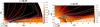 |
Fig. 1. Appearance of the inner disk in a zoomed snapshot in our magnetic simulation after T = 80 stellar rotations. The matter, is lifted from the disk into the accretion column, feeding it onto the stellar surface. The matter density is shown in logarithmic color grading in code units, with a sample of velocity vectors shown in two normalizations: since the velocity in the corona is much larger than in the disk, velocity vectors are shown with a different scaling in the disk and the corona, the units of the respective velocity vectors being shown in the legend at the bottom left of the figures. With the white solid lines is shown a sample of the poloidal magnetic field lines. The green solid line marks the position of the corotation radius. |
Both the equations and the resulting flow pattern seem too complicated to attempt an analytic solution. However, we would like to recover analytically the main features of the flow inside the disk, neglecting the stellar magnetosphere, except as an outer boundary condition on the disk solution, and ignoring the accretion column and the associated winds. Following the approach of KK00, where the solution for the viscous, hydrodynamical case of the thin accretion disk was derived, we analyze the equations for the magnetized, resistive accretion disk in the asymptotic expansion. For the first time, we consider also the energy equation in this context. This will help us to evaluate if omitting the heating terms in the energy equation is consistent with other equations. For comparison of the terms in the equations, the equations have to be written in normalized units.
In the asymptotic approximation, pioneered in the context of accretion disk by Regev (1983), all the variables are written in the Taylor expansion in the small coefficient ϵ, representing the dimensionless height of the disk  , with the tildes representing typical values, in this equation of the disk height H at radius R (as in the general discussion of asymptotic approximation in KK00 and also Umurhan et al. 2006). We can expand each variable X as X = X0 + ϵX1 + ϵ2X2 + ϵ3X3 + … and then, for each equation separately, consider all terms of the same order in ϵ.
We note that Eq. (1) involves the magnetic field components alone, while Eq. (2) only the fluid variables. All the other equations couple the fluid variables with the magnetic field. Even in the purely HD case (B = 0) the equations constitute a system of coupled partial differential equations, for four variables (density and the three components of velocity) if one assumes a polytropic equation of state. It is remarkable that it is possible to find an analytic solution to these equations in the HD case, and to derive clear-cut conclusions in the MHD case (B ≠ 0), as shown below.
In the case of a viscous HD disk, Eqs. (2) and (4) have been solved inside the disk (KK00). When a stellar magnetic field is present, the solution in the disk cannot be separated from the star-disk magnetosphere, because of the connection of the magnetic field in the corona with the field in the disk. In addition, a solution in the magnetosphere can itself be complicated by the reconnection events and outflows, and a back-reaction from the disk. Nonetheless, the asymptotic expansion method allows a derivation of constraints on the magnetic field inside the disk which are valid regardless of the field configuration outside it.
For the reader’s convenience, in Appendix A we give a step-by-step example of the asymptotic expansion in the equation of continuity, Eq. (2), together with the dimensionless thin-disk form of the remaining four equations of resistive MHD that we are solving, with a derivation of the conditions (obtained mostly from the zeroth and first order in ϵ) which the magnetic field should satisfy.
For instance, in the MHD case, just as in the HD KK00 results, for the lowest order terms in velocity we obtain Keplerian motion
 (6)
(6)
with the first order correction terms to the fluid variables vanishing (with the exception of radial velocity)
 (7)
(7)
In the HD case, the non-Keplerian velocity components (vr1, vz2, vφ2) can be obtained from the second order equations of momentum conservation, yielding the radial and azimuthal velocities, vr, rΩ, and from the equation of continuity yielding the vertical component of velocity, vz (KK00). Now, in the MHD case, the first two of these equations are coupled to the magnetic field components and their derivatives.
Order ϵ2:
 (8)
(8)
 (9)
(9)
We find (Appendix A) that the zeroth order components of the magnetic field all vanish, Bi0 = 0, i = r, z, φ, with  also zero. On the assumption–well borne out by our simulations–that magnetic pressure is not dominant,
  , the equations for the fluid variables through second order are exactly the same as for the HD case:
 (10)
(10)
 (11)
(11)
 (12)
(12)
Clearly, with the equations being the same, any difference between the HD and magnetic solution will depend on the boundary conditions. In the magnetic case, it is the magnetic field at the disk surface and at its inner edge that is producing the difference in numerical solutions (between the HD and MHD disks). We measure the overall effect of this difference by comparing the initial HD setup with the quasi-stationary magnetic solution from our simulations.
Indeed, the vertical disk profile in Hōshi (1977) and KK00 has been obtained by assuming that the disk density vanishes at the surface, ρ0 → 0 as z → h. If, instead, we supply at the disk surface a value at the boundary with the coronal density ρcd, we obtain:
![Mathematical equation: $$ \begin{aligned} \rho _0(r,z)=\left[\rho _{\rm cd}^{2/3}(r)+\frac{h^2(r)-z^2}{5r^3}\right]^{3/2}, \end{aligned} $$](/articles/aa/full_html/2023/10/aa40637-21/aa40637-21-eq17.gif) (13)
(13)
where h ≡ zd is the disk semi-thickness. The pressure and sound speed now become:
![Mathematical equation: $$ \begin{aligned}&P_0(r,z)=\left[\rho _{\rm cd}^{2/3}(r)+\frac{h^2(r)-z^2}{5r^3}\right]^{5/2},\end{aligned} $$](/articles/aa/full_html/2023/10/aa40637-21/aa40637-21-eq18.gif) (14)
(14)
![Mathematical equation: $$ \begin{aligned}&c_{\rm s{0}}(r,z)= \sqrt{\frac{5}{3}\left[\rho _{\rm cd}^{2/3}(r)+\frac{h^2(r)-z^2}{5r^3}\right]}. \end{aligned} $$](/articles/aa/full_html/2023/10/aa40637-21/aa40637-21-eq19.gif) (15)
(15)
Depending on the density contrast in the particular case under consideration, one can estimate the value of ρcd and obtain the relevant solution. The Hōshi (1977) solution is recovered by setting ρcd = 0.
In our case, since h ∝ r, we can write, with the proportionality constant h′, h = h′r. Assuming the corona at the surface of the disk to be in hydrostatic equilibrium, with ρcd = ρc0/r3/2 we can write:
![Mathematical equation: $$ \begin{aligned}&c_{\rm s0}^2(r,z)=\frac{5}{3} \left(\rho _{\rm cd}^{2/3}(r)+\frac{h^{\prime 2}r^2-z^2}{5r^3}\right)\nonumber \\&\qquad \quad =\frac{5}{3} \left(\frac{\rho _{\rm c0}^{2/3}(r)}{r}+\frac{h^{\prime 2}}{5r}-\frac{z^2}{5r^3}\right)\\&\qquad \quad =\frac{\zeta ^{-2}(r)}{3r}\left[1-\left(\zeta (r)\frac{z}{r}\right)^2\right] =\frac{1}{3r^3}\left[\bar{h}^2(r)-{z}^2\right],\nonumber \end{aligned} $$](/articles/aa/full_html/2023/10/aa40637-21/aa40637-21-eq20.gif) (16)
(16)
and similarly for the pressure and density, with
 (17)
(17)
Thus, the functional form of the vertical dependence of the density, pressure, and speed of sound is the same as in the case of ρcd = 0, with
 (18)
(18)
playing the role of the effective height squared.
On these grounds, of the disk solution through the second order in ϵ being independent of the magnetic field, we expect that if we knew the magnetic field configuration outside the disk, the magnetic field internal to the disk could be obtained by solving the induction equation alone on a fixed HD background of KK00 fluid solution, as was done in Naso et al. (2013), but with the external field furnishing here the boundary conditions on the surface of the disk. Of course, in fact we cannot know the external magnetic field without solving for the field inside the disk as well. As is well known, the initially dipole character of the stellar field undergoes a considerable rearrangement, leading to what is known as field inflation, whereby the magnetic field lines are pushed out, thus affecting the effective boundary conditions for the induction equation solution in the disk.
4. Results from numerical simulations compared with analytical results
In our numerical simulations, which are presented in detail in Čemeljić (2019) and briefly reviewed in Appendix B here, we consider a part of the star-disk system close to the central object, with the physical domain reaching only into the region of the disk where the Ohmic resistivity is the largest contributor to the dissipation in the induction equation. At the outer boundary we feed the disk with matter at a constant rate to allow the solution to reach a quasi-stationary state, as illustrated in Appendix B.
Starting from the analytical KK00 solution as an initial condition in the HD simulation, we obtain a numerical solution. Our computational domain reaches into the middle disk region, where the resistivity adds to the viscosity as a dissipation mechanism. This could make some of the assumptions from the purely HD disk implausible–with the help of numerical simulations we check whether or not this is true.
Our numerical solutions settle to a quasi-stationary state. A capture in our HD solution after 100 stellar rotations is shown in Fig. B.1. In this case, the accretion onto the star proceeds through the disk connected to the stellar equator. The mass flux onto the star and into the polar-origin wind during the simulation are shown in Fig. B.2.
The solution in the magnetic case is shown in Fig. 1. When the stellar dipole field is large enough, an accretion column is formed from the inner disk rim onto the stellar surface. The matter is lifted above the disk equatorial plane, following the magnetic field lines. The mass flux onto the star and into the wind is shown in Fig. B.3.
The quasi-stationary solution does not change much during the short interval of a few tens of stellar rotations which we capture in our simulations. The magnetic field and the accretion rate of the observed stars are practically constant during such an interval, so that it is sensible to compare the simulations with our time-independent analytical solutions, which–as it turned out–are a good representation of the simulation results. Comparing the quasi-stationary solutions in both the HD and MHD solutions, to the analytical solution, we find that the MHD and HD solutions follow the analytic solutions in the functional dependence of density and the components of velocity, only the proportionality constants change.
Before turning to a detailed comparison of the functional form F(r, z) of our numerical results with the predictions of asymptotic expansion, we verify that the magnetic field is compatible with the basic result of the analytical solution that the zeroth order magnetic field vanishes, B0 = 0 (“Overview” preceding Eq. (A.4)). Above the disk, and in the region between the star and the disk, the field can be strong, but the values of the magnetic field threading the thin disk are much lower. As seen in Fig. 2, in the middle part of the disk the field is two orders of magnitude smaller (dark blue region) than in the coronal region with the stellar wind above the disk. As can be seen in the bottom panel of the same figure, the magnetic force (gradient of the magnetic pressure) is negligible inside the disk in comparison to the other forces. Figures B.4 and B.5 present the Br, Bϕ, and Bz components, and the plasma β, respectively.
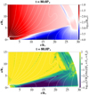 |
Fig. 2. Top panel: magnitude of the magnetic field in our simulation from Fig. 1, with logarithmic color grading in code units, and poloidal magnetic field lines shown with white solid lines. In the middle part of the disk, the magnetic field is two orders of magnitude smaller than in the corona, as predicted by our analytical solution in the disk, where the zeroth-order field vanishes, B0 = 0. The components are singled out in Fig. B.4. Near the boundaries, our analytical solution is less exact, as expected, since it is influenced by the magnetic field in the corona. Bottom panel: ratio of the gradient of magnetic pressure |

In Čemeljić (2019) we varied the stellar rotation rate, magnetic field strength, and resistivity in the disk and examined how the changes in results depend on those parameters. Here we focus on the comparison of the results with the conditions obtained from the analytical work. We then amend the lacking information in the analytical solution, merging our results from the analytical and numerical work, to obtain expressions which could be used as a model of a magnetized thin accretion disk4.
We output the results along the disk height at two positions in the disk: in the middle of the radial domain, at 15R⋆, which is in the outer region of our disk5 and in the inner region of the disk, closer to the star, at 6R⋆, about twice the corotation radius rcor = 2.9R⋆. We derive two sets of expressions along the vertical direction from those results, one at each distance from the star. Along the spherical radial direction, we output the results in the disk along a line near to the disk equator, and also along a line near to the disk surface. For each physical quantity, we verify if there is a unique solution throughout the disk.
Some quantities in the magnetic disk coincide with the HD solution more than others: the best match between our HD and MHD simulations is obtained for the vertical and radial profiles of the azimuthal velocity component (Fig. 3). We note (right panel) that the azimuthal velocity solution is uniform over a much larger range of z than in the assumed initial conditions, in which the corona was taken to be static for z > 2 at r = 15R⋆, i.e., above the initial height of the disk. Clearly, uniform rotation on vertical cylindrical surfaces is a property of the physical solution, and not an artefact of the initial conditions. At the same time the magnetic field lines are not vertical (left panel of Fig. 1). These two facts taken together show that the magnetic field configuration inside the disk is controlled by the flow, and not vice versa, a conclusion which is in agreement with our analytic considerations.
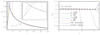 |
Fig. 3. Azimuthal velocity of thin disks from our simulations with Ω = 0.2 Ωms. As expected from theory, it closely follows the Keplerian curve and is uniform on cylinders (with corrections of order z2/r2). The disk-corona interface is at z ≈ 2. This and later figures exhibit values in the initial set-up (thin black solid line), and the quasi-stationary solutions in the numerical simulations in the HD (dot-dashed black line), and the MHD (long-dashed line) cases. Black, green, blue, and red colors correspond to stellar magnetic field strength (0.35, 0.7, 1.05, 1.4) |


In the magnetic case, the boundary conditions are different from the HD case firstly in that vφ/r has to match the rotation rate at the stellar surface, Ω⋆ = 0.2, and secondly that now the disk surface boundary condition at z = zd(r) is not that of vacuum. The former is responsible for6vφ → 0.2 cos θcap, as r → cos θcap (where θcap is the polar angle of the cap onto which the fluid is channeled by the magnetic field) and the overshoot of vφ above the Keplerian curve (clearly visible for the red dashed curve in Fig. 3), the latter for a different normalization of density and a different effective height of the disk.
With ρc0 typically ∼0.01, the height of the disk can be enhanced by several tens of percent (for h′∼0.1), as is the equatorial density through the ζ−2 pre-factor of Eq. (16). This is illustrated in Fig. 4 for the midplane density, and the vertical profile of the density at r = 15R⋆. Because of the difference in the influence of the boundary conditions in the magnetic case, both the radial and vertical profiles closer to the star, at r = 6R⋆ and at the disk surface are more noisy (Fig. 5).
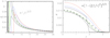 |
Fig. 4. Comparison of the matter density in the MHD simulation with analytic (triangles) and HD (dot-dashed) profiles. Left panel: radial dependence along the midplane, just above θ = 90°. Right panel: the profiles along the vertical line at r = 15R⋆. The legend is given in Fig. 3. |
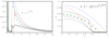 |
Fig. 5. Comparison of the matter density in the initial set-up (solid line) with the analytic profiles (triangles) and the quasi-stationary solutions in numerical simulations in the HD (dot-dashed line) and the MHD cases closer to the disk surface and the star. The solution is more noisy than in the previous figure. Left panel: density variation along the disk surface at θ = 83°. Right panel: density variation along a vertical line at r = 6R⋆; here, the trend of density increasing with the magnetic field is not maintained for the strongest fields, the red line being lower than the blue line. The meaning of the lines is the same as in Fig. 3. |
In agreement with our asymptotic expansion results, we find that the magnetic field does not strongly affect the flow inside the disk in the simulation. The agreement is seen by the good match between the analytic profiles (triangles) and the MHD results (lines) in Figs. 3–6. Accordingly, our simulated field configuration near the middle of the disk, around r = 15R⋆ in Fig. 1, is similar to the corresponding figure in Naso & Miller (2011, Fig. 3 there), even though they solved the induction equation on a background of constant flow of the thin HD disk solution, while our magnetic field configuration and the velocity field were solved for simultaneously (self-consistently).
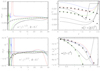 |
Fig. 6. Comparison of the r and z velocity components in the initial set-up (thin solid line) with the quasi-stationary solutions in the numerical simulations in the HD (dot-dashed line) and the MHD (long-dashed line) cases, with Ω = 0.2Ωms. The meaning of the lines is the same as in Fig. 3. Left panels: values averaged over 10 stellar rotations, to smooth out the oscillations. Right panels: values at r = 15R⋆. In the z-direction, an additional match is shown with squares in the cases with larger magnetic field. It has the same (analytically derived) functional dependence as shown with triangles for the smaller magnetic field, only the proportionality coefficient is different. |
If the magnetic field is influencing the solutions only quantitatively, but not qualitatively, the functional form of the fluid variables is expected to be as in KK00. Only the density will change, because of the inclusion of the corona-disk interface boundary conditions. The proper form for the density equation is given by the form of Eq. (16), leading to the substitution  , where
  , given by Eq. (18), is a slowly varying function of radius r, somewhat dependent on the magnetic field.
The analytic solutions are then:
![Mathematical equation: $$ \begin{aligned}&\rho (r,z)\propto \frac{1}{r^{3/2}}[\bar{h}^2-z^2]^{3/2},\end{aligned} $$](/articles/aa/full_html/2023/10/aa40637-21/aa40637-21-eq28.gif) (19)
(19)
![Mathematical equation: $$ \begin{aligned}&v_r(r,z)\propto \frac{1}{r^{1/2}}[1+(\zeta z)^2], \end{aligned} $$](/articles/aa/full_html/2023/10/aa40637-21/aa40637-21-eq29.gif) (20)
(20)
 (21)
(21)
 (22)
(22)
To investigate how much the magnetic solutions depart from the HD ones, and from the KK00 analytical solution, we directly compare the density and velocity profiles (Figs. 3–6). Since the analytic solutions are obtained in the cylindrical coordinates, which are more convenient to plot, we project our results from the simulations in spherical coordinates to the cylindrical coordinates. In all the cases, as in Fig. 4, we show (with triangle-symbol curves) the closest matches to the case with  , which is the medium value in our set of simulations. These are not formal best fits, but the functions in Eqs. (19)–(22) following from the analytic solution, with a normalization chosen to match the quasi-stationary solution. Inspection of the numerical solutions at r = 15R⋆ near the disk midplane, shown in Figs. 3–6, gives the following results:
– The radial dependence of density is practically the same in all simulations, and is equal to the non-magnetic case.
– Vertical velocity component vz also matches the corresponding non-magnetic solution very well, while the radial component vr is more noisy.
– The vertical dependence of density shows a trend: with larger magnetic field, the density is larger, so that it increases by up to about 25% with the doubling of the magnetic field strength. Higher above the disk midplane, the trend becomes more noisy.
– Both the radial and vertical dependence of the azimuthal velocity vφ is excellently fitted by Eq. (22), except at the very innermost parts of the disk, where the influence of the inner boundary condition is felt. In particular, there is no z dependence (rotation is uniform on cylinders), so that our solution behaves as predicted by the Taylor-Proudman theorem.
– The z dependence of the poloidal velocity components is fairly well described by Eqs. (20) and (21). There is also a clear trend in those components (as long as the geometry of the solutions stays the same; we describe solutions with different geometry directly below): with larger magnetic field, values are increasing. Higher above the disk midplane, the trend becomes more noisy.
In the solutions with larger magnetic field, the disk is pushed away, as shown in Fig. 7, and there is no accretion column: the geometry of the solution changed. The radial dependence departs from the predictions of Eqs. (21) and (22), so that the vz(r) plot (at a fixed value of θ) becomes very noisy, as do also the vr(r) curves for the two strongest magnetic field values (Fig. 6).
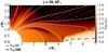 |
Fig. 7. Zoomed snapshot of the matter density in our simulation with large magnetic field, |

For the two lower B-field values, the vr(r) curves approximately track that of the HD simulation. In agreement with our analytic analysis that was discussed in Sect. 3, there is very little difference between the HD and these two MHD cases. Those three latter curves (black dot-dashed and black and green dashed lines, respectively, in Fig. 6) are significantly steeper than the  dependence of the thin disk without corona. It would seem that the radial dependence of vr is a result of the coronal pressure boundary condition on the disk surface. For a uniform and constant mass accretion rate, Ṁ = const, one has vr ∝ Ṁ/(rΣ), where Σ = ∫ρ dz = hρ + 𝒪(h3/r3) is the surface density of the disk in the upper half-plane. With ρ ∝ r−3/2, this gives close to the equatorial plane, up to terms 𝒪(h3/r3),
 (23)
(23)
In our simulation, instead of h ∝ r, we have an effective height  (Eq. (18)), which grows more rapidly than r, as can be verified by the concave shape of the disk in Figs. 1 and B.1, and therefore we expect the radial velocity to also vary more rapidly than r−1/2.
5. Torques on the star
Our simulation allows us to compute the torques on the star resulting from the disk-magnetosphere interaction including the effects of field inflation outside the disk, and the resulting change in the magnetic field threading the disk.
We begin with the HD case, where neither the star nor the disk has any appreciable magnetic field (Fig. 8). The torques are normalized to J⋆Ṁ/M⋆, with  the stellar moment of inertia computed in the shell approximation for the angular momentum of the star. As can be seen from the figure, the torques tend to a stationary value. The spin-up (or spin-down) timescale following from that value is on the order of ten accretion times M⋆/Ṁ.
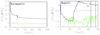 |
Fig. 8. Left panel: accretion (“material”) torque exerted on the non-magnetic star by the matter accreted from the disk (solid line), and the angular momentum loss rate in the wind (dashed line), in units of the stellar angular momentum multiplied by the accretion timescale. Right panel: torques exerted onto a magnetized star in the different components: flow in the wind (dashed green line), the contribution from the parts of the disk beyond Rcor (dotted blue line), and within Rcor (solid black line). The torque was measured in units of |
In the magnetized case, the time variation in the simulation of three significant components of the torque on the star are illustrated in the right panel in Fig. 8: the torque mediated by the open field lines, equal to the negative of the rate at which angular momentum is carried away by the wind, magnetic torque mediated by the closed field lines terminating on the disk beyond the co-rotation radius, and the torque exerted on the star by the disk inside the co-rotation radius. The latter component includes the difference in the rate of angular momentum carried by the accreting fluid as it leaves the disk and its value as it settles on the stellar surface (“material” torque), as well as the magnetic interactions between the star and the part of the disk that is inside the co-rotation radius. We have checked that the fluid settling on the star exerts a negligible torque (as its angular frequency is very close to that of the fairly slowly rotating star).
As in the non-magnetic case, the torques reach quasi-stationary values, with the exception of the wind torques, which are more noisy because of the ongoing reconnection events in the disk corona and occasional releases of energy as a result of instabilities near the stellar surface or along the outer disk boundary. The result we obtain is that, in the magnetic case, the magnitude of the net torque in our simulation is enhanced by an order of magnitude with respect to the HD case accretion torque. The timescale for change of stellar angular momentum is comparable to the accretion timescale,  .
.
6. Discussion and conclusions
We combine the analytical conditions obtained from the asymptotic approximation with the results from numerical simulations, to discuss solutions in resistive MHD for a thin accretion disk threaded by a magnetic field.
Interaction of the stellar magnetosphere with the accretion disk is of particular interest in models for torque-related changes in the spin of X-ray pulsars. The position of the accretion disk inner edge is consistent between different models within a factor of two, but the discussion is still open on the nature of magnetic interaction governing the stellar rotation. Naso et al. (2013) questioned the assumption that the contribution to the pulsar spin-up depends on the position of the accretion column inside of the disk truncation radius, but without a fully dynamical treatment only the induction equation was considered. Here we make a step closer to a full dynamical solution.
In the magnetic case, equations in the disk cannot be solved without knowing the solution in the corona above the disk and between the disk and the stellar surface. This is because of the connectivity of the magnetic field in the disk to the stellar surface. The solution is further complicated with the magnetic reconnection taking place in the corona. However, the numerical simulation takes account of the disk-magnetospheric interaction, so we solve self-consistently for the magnetic field configuration and for the disk fluid variables. From the simulations we obtain quasi-stationary solutions for a magnetic geometrically thin disk.
We also performed analytic calculation, solely within the disk, allowing a non-zero pressure at the disk-corona and magnetosphere interface. By performing an analysis of the relevant equations written as a power series in the small parameter  (the characteristic dimensionless disk thickness), we were able to show that the fluid variables satisfy the same equation of motion in the MHD and HD cases. The latter equations have been derived and solved for a polytropic disk in vacuum by KK00. Thus we compare our simulated solutions to the KK00 functional forms of the fluid variables. With the exception of radial velocity, which seems to show the greatest effect of non-vacuum boundary conditions (non-vanishing pressure at the disk-corona interface), the simulated solutions match the analytic expressions rather well.
We introduced the induction equation for the first time to the asymptotic expansion analysis. To check if our removal of the dissipative, heating terms, from the energy equation is consistent with other equations, we add the energy equation in the asymptotic expansion, also for the first time. As it turns out, the energy equation does not yield any new constraints on the asymptotic solution in the lowest orders. We find that the solutions obtained from the energy equation to lowest orders only give conditions on the magnetic field that already follow from the induction equation and the ∇ ⋅ B = 0 condition, which jointly imply Bi0 = 0.
Far from the inner boundary, say for r > 10R⋆ in our simulations, we find the following:
– Solution for the radial dependence of density is practically the same in non-magnetic and magnetic cases.
– The vertical dependence of density shows a trend: with larger magnetic field, the density is larger, so that it increases for up to about 25% with doubling of the magnetic field strength. Higher above the disk midplane, the trend becomes more noisy.
– The azimuthal velocity vφ is independent of the magnetic field, with both the radial and vertical dependence excellently fitted by Eq. (22), velocity inversely proportional to  , with no dependence on z.
– Vertical velocity component, vz, matches the corresponding non-magnetic solution very well. The radial component is more noisy, especially for high values of B, when the velocities are suppressed.
– The vertical (z) dependence of the poloidal velocity components is fairly well described by Eqs. (20) with a fitted constant ζ (cf. the prediction of Eq. (17) and (21)). There is a trend in the velocity components for those solutions which show the accretion column: the values increase for larger magnetic field. Higher above the disk midplane, the trend becomes more noisy.
– In the solutions with larger magnetic field, the disk is pushed away and there is no accretion column. Then the vr and vz radial dependence becomes very noisy.
– As it settles on the star, the fluid in our simulations exerts a negligible torque, since by then it almost co-rotates with the rotating star. The “material” accretion torque is mediated by the magnetic fields, as the fluid flows through the accretion column.
– The net spin-up torque in the magnetic case is an order of magnitude larger than in the HD case. The timescale for stellar angular change momentum is comparable to the accretion timescale.
In this paper, we compared the analytical solutions with numerical solutions in the cases with stellar rotation equal to 20% of the equatorial mass-shedding velocity. As shown in Čemeljić (2019), solutions with smaller stellar rotation rates follow similar trends, so that our conclusions should extend to such cases.
We end with some caveats: Our study here is limited to the values of the free parameters of viscosity and resistivity αv = αm = 1. We leave for a separate study an investigation of the solutions in other cases, in particular the case with a smaller viscosity parameter αv < 0.685, which shows a backflow region in the disk close to the disk equatorial plane (Mishra et al. 2023). We also leave for a separate study the cases with faster rotating stars, as they often exhibit axial jets and conical outflows, changing the geometry of the solutions.
We performed simulations in a quadrant of the meridional plane, enforcing at θ = π/2 (i.e., z = 0) boundary conditions consistent with equatorial plane reflection symmetry. The analytic calculation did not assume such a symmetry. However, some conclusions of the asymptotic expansion analysis (such as the vanishing of Bz0) relied on certain (finiteness) conditions applying in the lower half-plane, which is not present in our simulation. It remains to check the difference between solutions for simulations performed in the upper half and the full meridional plane.
For a review refer to the Appendix in Kluźniak & Rappaport (2007).
While stable solutions have recently been found in this regime, they are not geometrically thin (Lančová et al. 2019).
After the submission of this work, Mishra et al. (2020b); Mishra et al. (2023) have shown that for Prandtl numbers below a certain critical value backflow exists also in α-disks simulated with resistive MHD.
In Čemeljić et al. (2019) is presented one initial example of our search for numerical expressions from our simulation results, matching the analytical solutions.
The distance rm where the viscous torque vanishes defines a natural length scale  , as shown in KK00. The outer region of the disk is at a much larger radius.
We note that r is in units of R⋆ = 1.
The factor  is absorbed in B in the PLUTO code.
Acknowledgments
Work at CAMK is funded by the Polish NCN grant 2019/33/B/ST9/01564. MČ acknowledges the Czech Science Foundation (GAČR) grant No. 21-06825X and the support by the International Space Science Institute (ISSI) in Bern, which hosted the International Team project #495 (Feeding the spinning top) with its inspiring discussions. MČ developed the setup for star-disk simulations while in CEA, Saclay, under the ANR Toupies grant, and his collaboration with Croatian STARDUST project through HRZZ grant IP-2014-09-8656 is also acknowledged. During part of the text finalization MČ was supported by CAS President’s International Fellowship for Visiting Scientists (grant No. 2020VMC0002). VP’s work was partly funded by the Polish National Science Centre grant 2015/18/E/ST9/00580. We thank IDRIS (Turing cluster) in Orsay, France, ASIAA/TIARA (PL and XL clusters) in Taipei, Taiwan, and NCAC (PSK and CHUCK clusters) in Warsaw, Poland, for access to Linux computer clusters used for the high-performance computations. The PLUTO team is thanked for the possibility to use the code. We thank CAMK erstwhile Ph.D. student D. A. Bollimpalli and summer students F. Bartolić and C. Turski for developing the initial version of our Python scripts for visualization. We thank J. Horák for discussions of analytic solutions.
References
- Agapitou, V., & Papaloizou, J. C. B. 2000, MNRAS, 317, 273 [CrossRef] [Google Scholar]
- Aly, J. J. 1980, A&A, 86, 192 [Google Scholar]
- Borumand, M. 1997, PhD Thesis, University of Wisconsin, USA [Google Scholar]
- Chashkina, A., Lipunova, G., Abolmasov, P., & Poutanen, J. 2019, A&A, 626, A18 [NASA ADS] [CrossRef] [EDP Sciences] [Google Scholar]
- Čemeljić, M. 2019, A&A, 624, A31 [NASA ADS] [CrossRef] [EDP Sciences] [Google Scholar]
- Čemeljić, M., Parthasarathy, V., & Kluźniak, W. 2019, IAUS, 346, 264 [Google Scholar]
- Erkut, M. H., & Alpar, M. A. 2004, ApJ, 617, 461 [NASA ADS] [CrossRef] [Google Scholar]
- Fragile, P. C., Etheridge, S. M., Anninos, P., Mishra, B., & Kluźniak, W. 2018, ApJ, 857, 1 [CrossRef] [Google Scholar]
- Ghosh, P., & Lamb, F. K. 1979, ApJ, 234, 296 [Google Scholar]
- Ghosh, P., Lamb, F. K., & Pethick, C. J. 1977, ApJ, 217, 578 [Google Scholar]
- Hōshi, R. 1977, Prog. Theor. Phys., 58, 1191 [CrossRef] [Google Scholar]
- Igumenshchev, I. V., & Abramowicz, M. A. 2000, ApJS, 130, 463 [NASA ADS] [CrossRef] [Google Scholar]
- Kita, D. B. 1995, PhD Thesis, University of Wisconsin-Madison, USA [Google Scholar]
- Kluźniak, W., & Kita, D. 2000, ArXiv e-prints [arXiv:astro-ph/0006266] [Google Scholar]
- Kluźniak, W., & Rappaport, S. 2007, ApJ, 671, 1990 [CrossRef] [Google Scholar]
- Lančová, D., Abarca, D., Kluźniak, W., et al. 2019, ApJ, 884, L37 [CrossRef] [Google Scholar]
- Lee, W. H., & Ramirez-Ruiz, E. 2002, ApJ, 577, 893 [NASA ADS] [CrossRef] [Google Scholar]
- Mignone, A., Bodo, G., Massaglia, S., et al. 2007, ApJS, 170, 228 [Google Scholar]
- Mishra, B., Fragile, P. C., Johnson, L. C., & Kluźniak, W. 2016, MNRAS, 463, 3437 [NASA ADS] [CrossRef] [Google Scholar]
- Mishra, R., Čemeljić, M., Kluźniak, W., et al. 2020a, in XXXIX Polish Astronomical Society Meeting, ed. Małek, et al., 10, 147 [NASA ADS] [Google Scholar]
- Mishra, R., Čemeljić, M., & Kluźniak, W. 2020b, ArXiv e-prints [arXiv:2012.13194] [Google Scholar]
- Mishra, R., Čemeljić, M., & Kluźniak, W. 2023, MNRAS, 523, 4708 [NASA ADS] [CrossRef] [Google Scholar]
- Naso, L., & Miller, J. C. 2010, A&A, 521, A31 [NASA ADS] [CrossRef] [EDP Sciences] [Google Scholar]
- Naso, L., & Miller, J. C. 2011, A&A, 531, A163 [NASA ADS] [CrossRef] [EDP Sciences] [Google Scholar]
- Naso, L., Kluźniak, W., & Miller, J. C. 2013, MNRAS, 435, 2633 [CrossRef] [Google Scholar]
- Parfrey, K., & Tchekhovskoy, A. 2016, ApJ, 851, L34 [Google Scholar]
- Parfrey, K., Spitkovsky, A., & Beloborodov, A. M. 2016, ApJ, 822, 33 [NASA ADS] [CrossRef] [Google Scholar]
- Parfrey, K., Spitkovsky, A., & Beloborodov, A. M. 2017, MNRAS, 469, 3656 [Google Scholar]
- Philippov, A. A., & Rafikov, R. R. 2017, ApJ, 837, 101 [NASA ADS] [CrossRef] [Google Scholar]
- Powell, K. G., Roe, P. L., Linde, T. J., Gombosi, T. I., & De Zeeuw, D. L. 1999, J. Comput. Phys, 154, 284 [NASA ADS] [CrossRef] [Google Scholar]
- Rebusco, P., Umurhan, O. M., Kluźniak, W., & Regev, O. 2009, Phys. Fluids, 21, 076601 [NASA ADS] [CrossRef] [Google Scholar]
- Regev, O. 1983, A&A, 126, 146 [NASA ADS] [Google Scholar]
- Regev, O., & Gitelman, L. 2002, A&A, 396, 623 [NASA ADS] [CrossRef] [EDP Sciences] [Google Scholar]
- Romanova, M. M., Ustyugova, G. V., Koldoba, A. V., & Lovelace, R. V. E. 2012, MNRAS, 421, 63 [NASA ADS] [Google Scholar]
- Scharlemann, E. T. 1978, ApJ, 219, 617 [Google Scholar]
- Sdowski, A. 2016, MNRAS, 459, 4397 [CrossRef] [Google Scholar]
- Shakura, N. I., & Sunyaev, R. A. 1973, A&A, 24, 337 [NASA ADS] [Google Scholar]
- Shakura, N. I., & Sunyaev, R. A. 1976, MNRAS, 175, 613 [NASA ADS] [CrossRef] [Google Scholar]
- Tanaka, T. 1994, J. Comput. Phys., 111, 381 [Google Scholar]
- Umurhan, O. M., Nemirovsky, A., Regev, O., & Shaviv, G. 2006, A&A, 446, 1 [NASA ADS] [CrossRef] [EDP Sciences] [Google Scholar]
- Urpin, V. A. 1984, Astron. Zh., 61, 84, [Soviet Astron. 28, 50] [NASA ADS] [Google Scholar]
- Vasyliunas, V. M. 1975, Rev. Geophys. Space Phys., 13, 303 [CrossRef] [Google Scholar]
- Wang, Y.-M. 1996, ApJ, 465, L111 [NASA ADS] [CrossRef] [Google Scholar]
- Zanni, C., & Ferreira, J. 2009, A&A, 512, 1117 [CrossRef] [EDP Sciences] [Google Scholar]
Appendix A: Asymptotic expansion equations for a thin accretion disk
An example of the asymptotic approximation method is worked-out in detail in an example with the continuity equation, in which we derive all the terms to the second order. The remaining equations are derived by following the same method. We present second order equations of the set from Sect. 3. Unlike in the HD case (KK00), in general these cannot be solved without additional assumptions and/or boundary conditions.
In the hydrodynamic solution one can assume that the disk density decreases smoothly to zero towards the disk surface, which greatly simplifies the solution. In the magnetic case, the disk solution cannot be given without inclusion of the stellar corona, because of a magnetic connection with the star and a corona above the disk. To obtain a solution for the magnetic field penetrating the disk, we have to include the disk-corona boundary condition, which is unknown. Because of this, we can obtain only the most general conditions for the disk magnetic field from the equations. Full information about the magnetic field solution inside the disk can be obtained from our numerical simulations.
The normalization is defined with the following equations:  , so that
  , and then
  . Tildes denote characteristic values of the variables, and primes the scaled variables. Here,
  is the cylindrical radius, so
  is the characteristic azimuthal velocity. Further,
  ,
,  ,
,  ,
,  ,
,  ,
,  ,
,  . The magnetic field we normalize with the Alfvén speed
  as a characteristic speed, and
  . Then we have
  , and
, and  is the normalization for all the magnetic field components:
  ,
,  ,
,  .
.
The beta plasma parameter β = Pgas/Pmag = 8πPgas/B2. With P = Pgas we can write  , so that
  .
.
The viscosity scales with the sound speed as a characteristic velocity and the height of the disk H, so that the normalization for the kinetic viscosity is  , and then
  . Then
  . For the resistivity we choose the normalization with the Alfvén speed as a characteristic speed, so that
  . Then
  .
.
In the asymptotic approximation, following KK00, we write all the variables in the Taylor expansion with the coefficient of expansion  . For a variable X, we then have X = X0 + ϵX1 + ϵ2X2 + ϵ3X3 + …, and we can compare the terms of the same order in ϵ. We write the normalized equations of magnetic field solenoidality, continuity, induction, momentum, and energy density, i.e., Eqs. (1)–(5). For simplicity, in some cases we use the notation ∂x = ∂/∂x, and we drop all primes in the following (where all the variables are scaled, so no confusion can arise).
We will be searching for stationary solutions, so that the additional conditions are that of stationarity, ∂/∂t = 0, and axial symmetry ∂/∂φ = 0. We work in the cylindrical coordinates (r, z, φ).
Equation of continuity
We start from the continuity equation, Eq. (2) in Sect. 3:
In the stationary case, when ∂tρ = 0, and applying also the axi-symmetry condition ∂φ(ρv) = 0:
We can write the normalized equation, in which the terms can be written in the orders of a small parameter ϵ:
Removing the primes, we can write:
Writing the expansion in ϵ in each quantity, we obtain
![Mathematical equation: $$ \begin{aligned} \frac{\epsilon }{r}\partial _r[r(\rho _0+\epsilon \rho _1+\epsilon ^2\rho _2+\dots )({v}_{r0}+\epsilon {v}_{r1}+\epsilon ^2\rho _2+\dots )]\nonumber \\ +\partial _z[(\rho _0+\epsilon \rho _1+\epsilon ^2\rho _2+\dots )({v}_{z0}+\epsilon {v}_{z1}+\epsilon ^2{v}_{z2}+\dots )]=0.\nonumber \end{aligned} $$](/articles/aa/full_html/2023/10/aa40637-21/aa40637-21-eq75.gif)
From this we can write the term in the order zeroth order in ϵ as:
Order ϵ0:
 (A.1)
(A.1)
In a stationary solution, the disk midplane cannot be suffering a steady vertical drift, so we must have ρ0vz0 = 0 at z = 0. Since the product does not depend on z, we conclude that we must have vz0 = 0 throughout the disk (ρ0 ≠ 0).
Order ϵ1:
In the first order in ϵ we have:
 (A.2)
(A.2)
As we will see from the radial momentum equation, in the first order in ϵ, Eq. (A.27), we have vr0 = 0, so that here we have ∂z(ρ0vz1) = 0 ⇒ ρ0vz1 = const along z. Following the same argumentation as above, we conclude that vz1 = 0.
Order ϵ2:
In the second order in ϵ we have:
 (A.3)
(A.3)
Thus, if we find a solution for vr1, we will be able to determine the z dependence of vz2.
The same procedure is carried in each of the remaining equations of Sect. 3. In the following, we will often find that certain quantities are functions of the radial variable alone. In such cases we will denote a generic radial function as f(r), without implying any particular functional dependence on r, so that the results a = f(r), and b = f(r) do not imply a(r, z)≡b(r, z).
Overview
By parity arguments (KK00), or from a more formal derivation (Appendix A in Rebusco et al. 2009, or Borumand 1997), Ω1 = 0. Similarly, cs1=ρ1=vr0 = 0, for all r, z, with the last equation also expressly following from Eq. (A.27). It is easy to check that all the following equations are consistent with the zeroth order components of the magnetic field vanishing, Bi0 ≡ 0, i ∈ {r, z, φ}, as well as Bz1 ≡ 0.
We do not claim uniqueness of the presented solution, should the magnetic pressure turn out to be so dominant that  . However, on the assumption that
  it can be shown that Bi0 = 0 is the only solution satisfying reflection symmetry in the equatorial plane; the proof is outside the scope of this Appendix, but in the asymptotic expansion below we obtain conditions like ∂zBi0 = 0 or Bj0∂zBi0 = 0 for all the components of magnetic field, already implying that either Bj0 ≡ 0 or Bi0 = f(r). The same is obtained for B0 itself, and as a result the equation for the zeroth order vertical momentum also becomes independent of zeroth order total magnetic field B0. Such an outcome is also supported by the results of our numerical simulations.
Condition ∇⋅B = 0:
 (A.4)
(A.4)
Order ϵ0:
 (A.5)
(A.5)
Order ϵ1:
 (A.6)
(A.6)
Energy equation:
![Mathematical equation: $$ \begin{aligned}&\epsilon ^4 \tilde{R}^2\tilde{\Omega }^2 n\rho {v}_r\frac{\partial c_s^2}{\partial r}+\epsilon ^3\tilde{R}^2\tilde{\Omega }^2 n \rho {v}_z\frac{\partial c_s^2}{\partial z} +\epsilon \rho \tilde{{v}}^2{v}_z \frac{\partial {v}^2/2}{\partial z}\nonumber \\&+\epsilon ^2\rho \tilde{{v}}^2_{\rm A}{v}_r\frac{\partial {v}_{\rm A}}{\partial r} +\epsilon \rho \tilde{{v}}_{\rm A}^2{v}_z \frac{\partial {v}_{\rm A}^2}{\partial z} +\epsilon ^2\rho \tilde{{v}}^2{v}_r\frac{\partial {v}/2}{\partial r}\\&+\left[\epsilon ^2\rho \tilde{\Omega }^2 \tilde{R}^2\frac{{v}_r}{r^2}+\epsilon ^3\rho \tilde{\Omega }^2\tilde{R}^2\frac{{v}_z z}{r^3}\right] \left[1+\epsilon ^2\left(\frac{z}{r} \right)^2\right]^{-3/2}\nonumber \\&=\frac{\tilde{{v}}^2_{\rm A}B_r}{r} \left(\epsilon ^2 {v}_r B_r+\epsilon \Omega rB_\varphi \right)\nonumber \\&+\tilde{{v}}^2_{\rm A}\frac{\partial }{\partial r}\left(\epsilon ^2 {v}_r B_r^2 + \epsilon ^2 {v}_z B_z B_r +\epsilon \Omega r B_{\varphi } B_r \right) \nonumber \\&+\tilde{{v}}^2_{\rm A}\frac{\partial }{\partial z}\left( \epsilon {v}_r B_r B_z+ \epsilon {v}_z B_z^2+\Omega r B_{\varphi } B_z\right)\ .\nonumber \end{aligned} $$](/articles/aa/full_html/2023/10/aa40637-21/aa40637-21-eq84.gif) (A.7)
(A.7)
Order ϵ0:
 (A.8)
(A.8)
with the last but one equality following from Eq. (A.5), and the last from the logical implication of nonvanishing in the zeroth order of Ω from Eq. (A.22), the zeroth order radial momentum equation.
Order ϵ1:
 (A.9)
(A.9)
Vertical induction:
 (A.10)
Order ϵ0:
Because the radial and vertical components of velocity vanish in the zeroth order by Eqs. (A.1), (A.27), we are left with
 (A.11)
consistent with Br0 = 0.
Order ϵ1:
![Mathematical equation: $$ \begin{aligned}&{v}_{r1}\left(\frac{B_{z0}}{r}+\frac{\partial B_{z0}}{\partial r}\right) +B_{z0}\frac{{v}_{r1}}{\partial r}\nonumber \\&=\sqrt{\frac{2}{\gamma \tilde{\beta }}} \Bigg [\frac{\partial \eta _{\rm m0}}{\partial r}\Bigg (\frac{\partial B_{z0}}{\partial r} -\frac{\partial B_{r1}}{\partial z}\Bigg ) -\frac{\partial \eta _{\rm m1}}{\partial r}\frac{\partial B_{r0}}{\partial z}\\&+\frac{\eta _{\rm m0}}{r}\Bigg (\frac{\partial B_{z0}}{\partial r} -\frac{\partial B_{r1}}{\partial r}\Bigg ) -\eta _{\rm m0}\frac{\partial ^2 B_{r1}}{\partial r\partial z}\nonumber \\&-\eta _{\mathrm{m1}}\Bigg (\frac{1}{r}\frac{\partial B_{r0}}{\partial r}+\frac{\partial ^2B_{r0}}{\partial r\partial z}\Bigg )\Bigg ].\nonumber \end{aligned} $$](/articles/aa/full_html/2023/10/aa40637-21/aa40637-21-eq89.gif) (A.12)
(A.12)
With vanishing components of B0:
 (A.13)
Radial induction:
 (A.14)
Order ϵ0:
 (A.15)
Order ϵ1:
 (A.16)
Azimuthal induction:
 (A.17)
Order ϵ0:
 (A.18)
in agreement with Eq. (A.5).
Order ϵ1:
 (A.19)
which, with vanishing components of B0, becomes:
 (A.20)
Radial momentum:
![Mathematical equation: $$ \begin{aligned}&\epsilon ^2{v}_r\frac{\partial {v}_r}{\partial r}+\epsilon {v}_z\frac{\partial {v}_r}{\partial z}-\Omega ^2r =-\frac{1}{r^2} \left[1+\epsilon ^2\left(\frac{z}{r}\right)^2\right]^{-3/2}\nonumber \\&-\epsilon ^2n\frac{\partial c_{\rm s}^2}{\partial r}+\frac{2}{\gamma \tilde{\beta }}\frac{1}{\rho }\left(\epsilon ^2B_r\frac{\partial B_r}{\partial r} +\epsilon B_z\frac{\partial B_r}{\partial z}-\epsilon ^2\frac{B_\varphi ^2}{r}\right)\nonumber \\&-\frac{\epsilon ^2}{\gamma \tilde{\beta }}\frac{1}{\rho }\frac{\partial B^2}{\partial r}+ \frac{\epsilon ^3}{\rho r}\frac{\partial }{\partial r}\left(2\eta r\frac{\partial {v}_r}{\partial r}\right)+\frac{\epsilon }{\rho }\frac{\partial }{\partial z}\left(\eta \frac{\partial {v}_r}{\partial z}\right)\\&+\frac{\epsilon ^2}{\rho }\frac{\partial }{\partial z}\left(\eta \frac{\partial {v}_z}{\partial r}\right)-\epsilon ^3\frac{2\eta {v}_r}{\rho r^2}-\frac{2\epsilon ^3}{3\rho }\frac{\partial }{\partial r}\Bigg [\eta \frac{1}{r}\frac{\partial }{\partial r}\Big (r{v}_r\Big )\Bigg ]\nonumber \\&-\frac{2}{3}\frac{\epsilon ^2}{\rho }\frac{\partial }{\partial r}\left(\eta \frac{\partial {v}_z}{\partial z}\right).\nonumber \end{aligned} $$](/articles/aa/full_html/2023/10/aa40637-21/aa40637-21-eq98.gif) (A.21)
(A.21)
Here n is the polytropic index. In the case of adiabatic index γ = 5/3 for an ideal gas, we have n = 3/2.
Order ϵ0:
 (A.22)
Order ϵ1:
 (A.23)
Order ϵ2:
 (A.24)
Azimuthal momentum:
 (A.25)
Order ϵ0:
 (A.26)
which already follows from Eq. (A.22).
Order ϵ1:
 (A.27)
Since the last term vanishes by Eq. (A.8), and Ω1 = 0, we obtain vr0 = 0, necessarily. As expected, far from the inner and outer edges, radial flow in a thin disk is always subsonic.
Order ϵ2:
 (A.28)
Vertical momentum:
![Mathematical equation: $$ \begin{aligned} \epsilon {v}_r \frac{\partial {v}_z}{\partial r}&+ {v}_z \frac{\partial {v}_z}{\partial z} =-\frac{z}{r^{3}}\left[1+\epsilon ^{2}\left(\frac{z}{r}\right)^{2}\right]^{-3/2}\nonumber \\&-n\frac{\partial c_{\rm s}^2}{\partial z}+\frac{2}{\gamma \tilde{\beta }}\frac{1}{\rho }\left(\epsilon B_r\frac{\partial B_z}{\partial r}+B_z\frac{\partial B_z}{\partial z}\right)-\frac{1}{\gamma \tilde{\beta }} \frac{1}{\rho }\frac{\partial B^{2}}{\partial z}\nonumber \\&+\frac{2}{\rho }\frac{\partial }{\partial z}\left(\eta \frac{\partial {v}_z}{\partial z}\right) +\frac{\epsilon ^{2}}{\rho r}\frac{\partial }{\partial r}\left(r \eta \frac{\partial {v}_z}{\partial r}\right)\nonumber \\&-\frac{2}{3}\frac{\epsilon }{\rho }\frac{\partial }{\partial z}\Bigg [\frac{\eta }{r}\frac{\partial }{\partial r}\Big (r{v}_r\Big ) \Bigg ]-\frac{2}{3\rho }\frac{\partial }{\partial z}\left(\eta \frac{\partial {v}_z}{\partial z}\right)\nonumber \\&+\frac{\epsilon }{\rho r} \frac{\partial }{\partial r}\left(\eta r\frac{\partial {v}_r}{\partial z}\right) \ . \end{aligned} $$](/articles/aa/full_html/2023/10/aa40637-21/aa40637-21-eq106.gif) (A.29)
(A.29)
Order ϵ0:
 (A.30)
With B0 = 0, we have
 (A.31)
which is the vertical hydrostatic equilibrium equation, with no contribution from the magnetic pressure.
Order ϵ1:
![Mathematical equation: $$ \begin{aligned}&\frac{2}{\gamma \tilde{\beta }} \left[B_{z0}\frac{\partial B_{z1}}{\partial z} -\frac{\partial }{\partial z}\left(B_0B_1\right)\right] -\frac{2}{3r}\frac{\partial }{\partial z}\left[\eta _0 \frac{\partial }{\partial r}\left(r{v}_{r1}\right)\right]\nonumber \\&+\frac{1}{r}\frac{\partial }{\partial r} \left(\eta _0r\frac{\partial {v}_{r1}}{\partial z}\right)=0. \end{aligned} $$](/articles/aa/full_html/2023/10/aa40637-21/aa40637-21-eq109.gif) (A.32)
(A.32)
With Bz0 = B0 = 0 we obtain:
![Mathematical equation: $$ \begin{aligned} \frac{\partial }{\partial z} \left[\eta _0\frac{\partial }{\partial r}\left(r{v}_{r1}\right)\right] =\frac{3}{2}\frac{\partial }{\partial r} \left(\eta _0r\frac{\partial {v}_{r1}}{\partial z}\right). \end{aligned} $$](/articles/aa/full_html/2023/10/aa40637-21/aa40637-21-eq110.gif) (A.33)
(A.33)
Appendix B: Numerical setup
In Čemeljić (2019), following Zanni & Ferreira (2009) we solve the non-ideal MHD equations using the PLUTO (v.4.1) code (Mignone et al. 2007) in the spherical grid. The resolution is R × θ = (217 × 100) grid cells, in a logarithmically stretched radial grid and in the first quarter of the meridional plane in a uniform polar-angle grid, θ ∈ [0, π/2]. In our numerical upper half-plane simulation we took reflective boundary conditions at z = 0, in agreement with reflection symmetry in the equatorial plane.
The grid resolution is chosen so that the accretion column width is captured with more than 10 grid cells, and radially logarithmic stretched grid gives the largest precision where it is needed, close to the disk inner radius. Simulations with half this resolution in the latitudinal direction and a corresponding logarithmic spacing, R × θ = (109 × 50) (to maintain the square shape of the computation grid cells) give qualitatively similar results. In simulations with radial extension of the computational box increased 10-fold, up to Rmax = 300 R⋆, where we performed long lasting simulations, for up to 5000P⋆, the results are also qualitatively similar to the results obtained in the higher resolution runs reported here.
The viscosity and resistivity are parameterized by the Shakura & Sunyaev (1973)α-prescription as proportional to  . For the magnetic field, a split-field method is used, so that we evolve in time only changes from the initial stellar magnetic field (Tanaka 1994; Powell et al. 1999), with the constrained transport method used to maintain ∇ · B = 0. Simulations were performed using the second-order piecewise linear reconstruction and an approximate Roe solver. The second-order time-stepping (RK2) was employed.
As an initial condition we use the HD solution of a KK00 disk, adding a hydrostatic corona and the stellar magnetic dipole field atop a rotating stellar surface. We derive the custom boundary condition for Bφ from the condition for the stellar surface as a rotating perfect conductor. During the simulation the corona and the magnetic field evolve, exerting pressure on the disk surface.
Our computational domain reaches into the middle disk region, where the resistivity adds to the viscosity as a dissipation mechanism. This could make some of the assumptions from the purely HD disk implausible—with the help of numerical simulations we check whether or not this is true. A capture in our HD solution after 100 stellar rotations is shown in Fig. B.1. In this case, the accretion onto the star goes through the disk connected to the stellar equator. The mass flux onto the star and into the stellar wind during the simulation are shown in Fig. B.2.
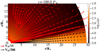 |
Fig. B.1. Capture into our hydrodynamic simulation after T = 100 stellar rotations. The matter density is shown in logarithmic color grading in code units, with a sample of velocity vectors. Colors and vectors have the same meaning as in Fig. 1. |
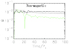 |
Fig. B.2. Illustration of the quasi-stationarity of our solution in the HD case, with the mass flux computed in the code units |
Here we present the results in our viscous HD and non-ideal MHD numerical simulations in the physical domain reaching 30 stellar radii, Rmax = 30R⋆, with the stellar rotation rate Ω⋆ = 0.20 Ωms, at 20% of the equatorial mass-shedding (“break-up”) limit, equal to the Keplerian angular velocity at the stellar equator  . Thus, the corotation radius is
  . The anomalous viscosity parameter (much larger than their microscopic equivalent, assuming that dissipation is a result of turbulence) is taken to be αv = 1. It is a free parameter in the simulation. In the magnetic case we add the stellar dipole field and the resistivity parameter αm = 1, so that the magnetic Prandtl number Pm = 2αv/(3αm) = 0.67.
In Fig. B.4 are shown the components of the magnetic field, to illustrate the outcome summarized in Fig. 2 that magnetic field does not influence the solution in the disk in the lowest, zeroth order. The large value of plasma-β in the disk middle part, as shown in Fig. B.5, also supports this conclusion.
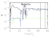 |
Fig. B.3. Illustration of quasi-stationarity in our magnetic case solutions, in the same (code) units as in Fig. B.2. Shown is the mass flux in the various components of the flow through the disk at r = 15R⋆ (solid black line), onto the stellar surface (dotted blue line), and into the magnetospheric wind (dashed green line). Vertical thin lines mark the interval in which we take the average for quasi-stationary solution. |
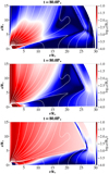 |
Fig. B.4. Cylindrical components Br, Bz, and Bφ of the magnetic field in our simulation from Fig. 1, shown with logarithmic color grading in code units. The total field is shown in Fig. 2. In the middle part of the disk, the magnetic field is orders of magnitude smaller than in the corona, as predicted by our analytical solution in the disk. Magnetic field is dominant outside of the disk, inside the disk it hardly influences the flow. |
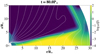 |
Fig. B.5. Plasma |

These simulations can be applied to any of a number of objects. Here we are interested in neutron stars in X-ray pulsars. Much higher field values, as would be needed for the classic X-ray pulsars such as Her X-1, would require a much shorter time-step and make the simulation prohibitively expensive. As already remarked, one of the motivations of our analytic study is to confidently allow our results to be scaled to stronger magnetic fields.
For neutron stars, with mass of M⋆ = 1.4M⊙, radius R⋆ = 10 km and with the disk density unit chosen as ρd0 = 5 × 10⁻⁶g/cm3, from Ṁ0 =  we have Ṁ0 = 5.7×10⁻⁷ M⊙/yr as our unit of mass accretion. The initial coronal density was defined as a free parameter in the code, ρc0 = 0.01ρd0. The unit of the scaled magnetic field is then
  =
= = 2.93×10⁷ G. The free parameter μ=
 (0.35, 0.7, 1.05, 1.4) for the magnetic field strength7 gives the stellar field B⋆=(0.36, 0.73, 1.09, 1.45)×108 G, close to the accepted value for millisecond accreting pulsars. In the Classical T-Tauri star cases, the stellar mass is M⋆ = 0.5M⊙, radius R⋆ = 2R⊙, and we choose the stellar angular velocity of 0.2 Ωms, which gives the stellar rotation period of P⋆ = 2π/Ω⋆ = 2.32 days. If we choose the same mass accretion unit as above, we have ρd0 ∼ 8.5 × 10⁻¹¹g/cm3, and
  =
= 0.2 kG, and the stellar fields with the same free parameters μ as above would produce B⋆≃(0.25, 0.5, 0.75, 1) kG, realistic for the YSO cases. A table for rescaling to different types of objects is given in Čemeljić (2019), where a parameter study was performed with the same set-up.
All Figures
|
Fig. 1. Appearance of the inner disk in a zoomed snapshot in our magnetic simulation after T = 80 stellar rotations. The matter, is lifted from the disk into the accretion column, feeding it onto the stellar surface. The matter density is shown in logarithmic color grading in code units, with a sample of velocity vectors shown in two normalizations: since the velocity in the corona is much larger than in the disk, velocity vectors are shown with a different scaling in the disk and the corona, the units of the respective velocity vectors being shown in the legend at the bottom left of the figures. With the white solid lines is shown a sample of the poloidal magnetic field lines. The green solid line marks the position of the corotation radius. |
| In the text | |
|
Fig. 2. Top panel: magnitude of the magnetic field in our simulation from Fig. 1, with logarithmic color grading in code units, and poloidal magnetic field lines shown with white solid lines. In the middle part of the disk, the magnetic field is two orders of magnitude smaller than in the corona, as predicted by our analytical solution in the disk, where the zeroth-order field vanishes, B0 = 0. The components are singled out in Fig. B.4. Near the boundaries, our analytical solution is less exact, as expected, since it is influenced by the magnetic field in the corona. Bottom panel: ratio of the gradient of magnetic pressure |
| In the text | |
|
Fig. 3. Azimuthal velocity of thin disks from our simulations with Ω = 0.2 Ωms. As expected from theory, it closely follows the Keplerian curve and is uniform on cylinders (with corrections of order z2/r2). The disk-corona interface is at z ≈ 2. This and later figures exhibit values in the initial set-up (thin black solid line), and the quasi-stationary solutions in the numerical simulations in the HD (dot-dashed black line), and the MHD (long-dashed line) cases. Black, green, blue, and red colors correspond to stellar magnetic field strength (0.35, 0.7, 1.05, 1.4) |
| In the text | |
|
Fig. 4. Comparison of the matter density in the MHD simulation with analytic (triangles) and HD (dot-dashed) profiles. Left panel: radial dependence along the midplane, just above θ = 90°. Right panel: the profiles along the vertical line at r = 15R⋆. The legend is given in Fig. 3. |
| In the text | |
|
Fig. 5. Comparison of the matter density in the initial set-up (solid line) with the analytic profiles (triangles) and the quasi-stationary solutions in numerical simulations in the HD (dot-dashed line) and the MHD cases closer to the disk surface and the star. The solution is more noisy than in the previous figure. Left panel: density variation along the disk surface at θ = 83°. Right panel: density variation along a vertical line at r = 6R⋆; here, the trend of density increasing with the magnetic field is not maintained for the strongest fields, the red line being lower than the blue line. The meaning of the lines is the same as in Fig. 3. |
| In the text | |
|
Fig. 6. Comparison of the r and z velocity components in the initial set-up (thin solid line) with the quasi-stationary solutions in the numerical simulations in the HD (dot-dashed line) and the MHD (long-dashed line) cases, with Ω = 0.2Ωms. The meaning of the lines is the same as in Fig. 3. Left panels: values averaged over 10 stellar rotations, to smooth out the oscillations. Right panels: values at r = 15R⋆. In the z-direction, an additional match is shown with squares in the cases with larger magnetic field. It has the same (analytically derived) functional dependence as shown with triangles for the smaller magnetic field, only the proportionality coefficient is different. |
| In the text | |
|
Fig. 7. Zoomed snapshot of the matter density in our simulation with large magnetic field, |
| In the text | |
|
Fig. 8. Left panel: accretion (“material”) torque exerted on the non-magnetic star by the matter accreted from the disk (solid line), and the angular momentum loss rate in the wind (dashed line), in units of the stellar angular momentum multiplied by the accretion timescale. Right panel: torques exerted onto a magnetized star in the different components: flow in the wind (dashed green line), the contribution from the parts of the disk beyond Rcor (dotted blue line), and within Rcor (solid black line). The torque was measured in units of |
| In the text | |
|
Fig. B.1. Capture into our hydrodynamic simulation after T = 100 stellar rotations. The matter density is shown in logarithmic color grading in code units, with a sample of velocity vectors. Colors and vectors have the same meaning as in Fig. 1. |
| In the text | |
|
Fig. B.2. Illustration of the quasi-stationarity of our solution in the HD case, with the mass flux computed in the code units |
| In the text | |
|
Fig. B.3. Illustration of quasi-stationarity in our magnetic case solutions, in the same (code) units as in Fig. B.2. Shown is the mass flux in the various components of the flow through the disk at r = 15R⋆ (solid black line), onto the stellar surface (dotted blue line), and into the magnetospheric wind (dashed green line). Vertical thin lines mark the interval in which we take the average for quasi-stationary solution. |
| In the text | |
|
Fig. B.4. Cylindrical components Br, Bz, and Bφ of the magnetic field in our simulation from Fig. 1, shown with logarithmic color grading in code units. The total field is shown in Fig. 2. In the middle part of the disk, the magnetic field is orders of magnitude smaller than in the corona, as predicted by our analytical solution in the disk. Magnetic field is dominant outside of the disk, inside the disk it hardly influences the flow. |
| In the text | |
|
Fig. B.5. Plasma |
| In the text | |
Current usage metrics show cumulative count of Article Views (full-text article views including HTML views, PDF and ePub downloads, according to the available data) and Abstracts Views on Vision4Press platform.
Data correspond to usage on the plateform after 2015. The current usage metrics is available 48-96 hours after online publication and is updated daily on week days.
Initial download of the metrics may take a while.