© C. Peralta et al. 2022

1. Introduction

A fundamental problem in accretion disks is the generation of structured, large-scale magnetic fields, which are a key element in the rich dynamics observed in these systems, including the generation of jets and outflows. A mechanism that is thought to be responsible for the generation and sustenance of these magnetic fields is an internal disk dynamo. On the one hand, dynamo theories involve mechanisms, such as the α effect, that have to be modeled and parameterized, which also holds for the (turbulent in general) diffusivity coefficients required in the model. On the other hand, due to the huge number of degrees of freedom involved, magnetohydrodynamics (MHD) numerical approaches are limited to simulating only the large scales, requiring the modeling of the effects of smaller scales.

In recent years, different numerical dynamo simulations made it possible to quantitatively study the generation of magnetic fields in accretion disks. Stepanovs et al. (2014) solved an axisymmetric α² − Ω dynamo using the code PLUTO. They showed that this type of dynamo can generate a large-scale magnetic field and a jet, even with a low magnetization, which allows using a hydrodynamic model to describe the disk. Furthermore, with a time-dependent α, it is possible to reproduce the observed episodic ejections (Burrows et al. 1996).

Hogg & Reynolds (2018) studied the influence of the disk thickness on the large-scale magnetic dynamo. They solved ideal MHD equations in conservative form with a pseudo-Keplerian potential, allowing for a flux through the surface of the disk. Their results showed that in thick disks with ratios $\frac{H}{r}\sim 0.4,$ the dynamo is less effective than in thin disks with ratios $\frac{H}{r}\sim 0.01$. The reason is that in the disks with higher ratios, the fluctuations in B_ϕ are more rapid, disorganized, and chaotic than in disks with lower ratios, indicating stronger turbulent fluctuations and consequently stronger dissipation.

On the other hand, Latif & Schleicher (2016) studied a magnetic field generated by a small-scale dynamo, and amplified it by an α − Ω dynamo. They considered a classic, primordial disk around a 10 M_⊙ star, with external radius r_e ∼ 1000 AU, and found that amplification is more effective if r <  10 AU, obtaining magnetic fields in the range 10⁻² − 10² G. Moreover, the magnetic field was coherent up to r ∼ 100 AU, which corresponds to the region that contributes more to the generated jet. The results about the distribution of the magnetic field were studied by Li & Cao (2016), who imposed an external magnetic field to search for a relation between this field and the field in the inner region of the disk. They used a model based on an iterative solution of the integro-differential form of the induction equation, and found that the external field helps to generate a large-scale magnetic field in the disk. Furthermore, even if the external field has a moderate intensity, it can result in a high-intensity field near the internal radius of the disk, and it can induce an inclination of the magnetic lines to the surface of the disk, which helps to launch outflows. As this result shows, the external magnetic field seems to be crucial for the topology of the magnetic field inside the disk, independently of the involved amplification mechanism.

We study the results obtained using a large-scale model of an axisymmetric dynamo with feedback effects developed in Sraibman & Minotti (2016, 2019), which realistically reproduces the magnetic dynamics of the Sun (Sraibman & Minotti 2019) and other stars (Buccino et al. 2020), including cycle times, magnetic field amplitudes, and phases. We also include a magnetosphere described by the Grad–Shafranov equation, in which the function relating the axial current to the magnetic flux is not prescribed, but determined self-consistently by matching conditions between disk and magnetosphere.

In Sect. 2 we recall the main aspects of the dynamo model. In Sects. 3 and 4 we present the most important aspects of disk, the magnetosphere and the main parameters selected for this work. In Sect. 5 we present the main results, which are discussed further in Sect. 6.

2. Dynamo model

We include here a short description of the model developed in Sraibman & Minotti (2016) and Sraibman & Minotti (2019), which corresponds to the evolution equation of the large-scale magnetic field, including feedback effects by the Lorentz force on the mass flow. The large-scale equations are obtained by averaging the original MHD evolution equations on local (running) volumes of linear scale λ. An axially symmetric system is finally obtained by further averaging on the azimuthal angle ϕ about the rotation axis z. In spherical coordinates r, θ, ϕ, the large-scale magnetic field B is determined by its azimuthal component B_ϕ(r, θ, t) and that of the vector potential of the zonal magnetic field A_ϕ(r, θ, t),

$$\begin{array}{c}\hfill \mathbf{B}=\mathrm{\nabla }\times \left(A_{\varphi }{\mathit{e}}_{\varphi }\right)+B_{\varphi }{\mathit{e}}_{\varphi }.\end{array}$$(1)

The evolution equations obtained after averaging on running volumes of linear scale λ, and azimuthal angle are

$$\begin{array}{c}\hfill \frac{\partial A_{\varphi }}{\partial t}=U_r{B}_{\theta }-U_{\theta }{B}_r+\eta ({\mathrm{\nabla }}^2{A}_{\varphi }-\frac{A_{\varphi }}{r^2{sin}^2\theta })+\alpha B_{\varphi }+S_{\varphi },\end{array}$$(2)

and

$$\begin{array}{c}\hfill \frac{\partial B_{\varphi }}{\partial t}=[\mathrm{\nabla }\times (\mathit{U}\times \mathbf{B}-\eta \mathrm{\nabla }\times \mathbf{B})+\mathrm{\nabla }\times \mathit{S}]·{\mathit{e}}_{\varphi },\end{array}$$(3)

where η is a prescribed small-scale magnetic diffusivity, α is the function corresponding to the α effect, and U is the axisymmetric large-scale velocity. This velocity includes a meridional velocity component U_m and an azimuthal component U_ϕ = Ω(r,θ)rsinθ, where Ω(r,θ) is the local large-scale angular velocity. In these equations, S corresponds to the electromotive tensor and diffusivity tensor effects, which are obtained through the formalism in Minotti (2000), and are given in terms of expressions of U and B, reproduced in the appendix. A modification ${\mathit{U}}_{\mathrm{m}}^{(1)}$ to the base meridional flow ${\mathit{U}}_{\mathrm{m}}^{(0)}$ is generated by the magnetic field through the Lorentz force. The corresponding equation for this term is

$$\begin{array}{c}\hfill \rho {\mathit{U}}_{\mathrm{m}}^{(1)}·\mathrm{\nabla }\left(\mathrm{\Omega }{r}^2{sin}^2\theta \right)=\frac{1}{{\mu }_0}[\mathrm{\nabla }\times \left(A_{\varphi }{\mathit{e}}_{\varphi }\right)]·\mathrm{\nabla }(rsin\theta B_{\varphi }),\end{array}$$(4)

together with the meridional mass flow conservation, written in terms of a stream function ψ⁽¹⁾,

$$\begin{array}{c}\hfill \rho {\mathit{U}}_{\mathrm{m}}^{(1)}=\frac{1}{rsin\theta }\mathrm{\nabla }{\psi }^{\left(1\right)}\times {\mathit{e}}_{\varphi }.\end{array}$$(5)

The α function is obtained self-consistently and is related to the radial cylindrical component of the mean vorticity, ω_s,

$$\begin{array}{c}\hfill \alpha =\frac{{\lambda }^2\varkappa }{12s}{\omega }_s,\end{array}$$(6)

with 0 <  𝜘 ≦ 1 an adjustable parameter of the model, and s the distance to the rotation axis z. The main contribution to ω_s comes from the differential rotation of the disk,

$$\begin{array}{c}\hfill {\omega }_s^{(0)}=-\frac{\partial U_{\varphi }^{(0)}}{\partial z}=sin\theta [sin\theta \frac{\partial \mathrm{\Omega }}{\partial \theta }-rcos\theta \frac{\partial \mathrm{\Omega }}{\partial r}],\end{array}$$(7)

and the correction due to the velocity modification by the magnetic field is given by (cylindrical coordinates are used to facilitate the notation)

$$\begin{array}{c}\hfill \frac{\partial {\omega }_s^{(1)}}{\partial t}+U_s^{(0)}(\frac{\partial {\omega }_s^{(1)}}{\partial s}+\frac{{\omega }_s^{(1)}}{s})+U_z^{(0)}\frac{\partial {\omega }_s^{(1)}}{\partial z}+{\omega }_s^{(1)}\frac{\partial U_z^{(0)}}{\partial z}=K,\end{array}$$(8)

where

$$\begin{array}{c}\hfill K={\omega }_z^{(0)}\frac{\partial U_s^{(1)}}{\partial z}-{\omega }_s^{(0)}\frac{\partial U_z^{(1)}}{\partial z}-U_s^{(1)}(\frac{\partial {\omega }_s^{(0)}}{\partial s}+\frac{{\omega }_s^{(0)}}{s})-U_z^{(1)}\frac{\partial {\omega }_s^{(0)}}{\partial z}.\end{array}$$(9)

In this way, the α coefficient is obtained from the solution to Eq. (8) with K given by Eq. (9), together with expression (7), resulting in

$$\begin{array}{c}\hfill \alpha =\frac{{\lambda }^2\varkappa }{12s}[{\omega }_s^{(0)}+{\omega }_s^{(1)}].\end{array}$$(10)

This set of equations constitutes the dynamo model, which requires as input the hydrodynamic disk structure in terms of the basic mass flow, the density distribution, and the small-scale diffusivity η.

3. Accretion disk and magnetosphere models

We considered as the base hydrodynamic structure of the disk that of the Shakura–Sunyaev model (Shakura & Sunyaev 1973). The density is given by the expression

$$\begin{array}{c}\hfill \rho =\frac{\dot{M}}{6\pi \nu H}(1-\sqrt{\frac{r_{\ast }}{r}}){\mathrm{e}}^{-\frac{r^2{cos}^2\theta }{2H^2}},\end{array}$$(11)

where ν is the turbulent viscosity, and H is the half-thickness of the disk,

$$\begin{array}{c}\hfill H=\gamma r\end{array}$$(12)

with γ >  0 a dimensionless factor. The viscosity ν can be expressed as a function of the sound speed in the medium, C_s, and the dimensionless parameter a as

$$\begin{array}{c}\hfill \nu =aH{C}_s.\end{array}$$(13)

We set the parameter a = 0.01, a typical value that implies an evolutionary timescale of the system close to 1 Myr (Dominik 2015).

Considering the material in the thin accretion disk modeled as an ideal gas, we can write the density as a function of the radius only as

$$\begin{array}{c}\hfill \rho =\frac{\dot{M}}{6\pi {\gamma }^2{r}^{2}a}\sqrt{\frac{m_{\mathrm{i}}}{k_{\mathrm{B}}T}},\end{array}$$(14)

where T is the temperature.

We considered the quasi-Keplerian accretion disk to be located between an internal radius r_i and an external radius r_e. The angular velocity was considered to be Keplerian, but U has components in e_r and e_θ given by

$$\begin{array}{cc}& U_r=-\frac{3}{2}\frac{\nu }{r}{(1-\sqrt[]{\frac{r_{\ast }}{r}})}^{-1},\hfill \end{array}$$(15)

$$\begin{array}{cc}& U_{\theta }=U_r\frac{r}{H}\frac{\partial H}{\partial r}cos\theta .\hfill \end{array}$$(16)

The small-scale magnetic diffusivity was modeled using Smagorinsky’s expression (Scotti et al. 1993),

$$\begin{array}{c}\hfill \eta (r,\theta )=C_k^2\mathrm{\Delta }r\mathrm{\Delta }\theta r\sqrt{2S_{\mathit{kl}}{S}_{\mathit{kl}}},\end{array}$$(17)

where C_k is the Smagorinsky coefficient, S_kl is the large-scale rate of strain due to the meridional and azimuthal large-scale velocity field, and Δr and Δθ the local radial and latitudinal grid sizes, respectively.

Boundary conditions for the magnetic field in the disk-magnetosphere interface are required. Using 1 as a lower index for quantities inside the accretion disk and 2 for those in the magnetosphere, the boundary conditions at the interface can be written as

$$\begin{array}{cc}& A_{\varphi 1}=A_{\varphi 2},\hfill \end{array}$$(18a)

$$\begin{array}{cc}& B_{\varphi 1}=B_{\varphi 2}.\hfill \end{array}$$(18b)

These conditions also apply at the interface between the low-density region and the magnetosphere. The necessary continuity of the azimuthal component of the potential vector A_ϕ across the disk-magnetosphere interface also ensures the required condition that B_θ is continuous across this interface. Moreover, because a magnetosphere with very high electric conductivity is in contact with the disk, the continuity of the tangential electric field across the boundary disk-magnetosphere ensures a vanishing tangential (radial) volume density of the electric current in the disk at the interface because the disk has a finite electrical conductivity. This is so because, being threaded by the magnetic field of the disk, the fluid element of the magnetosphere in contact with the disk is assumed to corotate with it, which together with the continuity of B_θ, ensures that the radial electric field in the fluid frame is zero at both sides of the interface. The vanishing of this current leads then, via the Ampère equation, to the condition for the azimuthal component of the magnetic field B_ϕ in the disk, at the disk surface,

$$\begin{array}{c}\hfill \frac{\partial }{\partial \theta }(B_{\varphi }sin\theta )=0.\end{array}$$(19)

The azimuthal component of the electric current cannot be considered zero at the disk side of the magnetosphere-disk interface because the radial velocity of fluid elements at each side can be different in principle. However, the assumption of no surface current density at the interface suffices to ensure continuity of ∂A_ϕ/∂θ at this boundary, which is an additional condition required to match disk and magnetosphere solutions.

The numerical method for solving the internal problem of the accretion disk is the same as was used in Sraibman & Minotti (2016). The main difference is that the solution needs to be matched to the external solution corresponding to the magnethosphere, described by the Grad–Shafranov equation, given in spherical coordinates as

$$\begin{array}{c}\hfill \frac{{\partial }^2\mathrm{\Psi }}{\partial r^2}+\frac{1}{r^2}\frac{{\partial }^2\mathrm{\Psi }}{\partial {\theta }^2}-\frac{1}{r^{2}tan\theta }\frac{\partial \mathrm{\Psi }}{\partial \theta }=-\frac{{\mu }_0^2}{4{\pi }^2}I(\mathrm{\Psi })\frac{\partial I(\mathrm{\Psi })}{\partial \mathrm{\Psi }},\end{array}$$(20)

where Ψ = A_ϕrsinθ and $I=\frac{1}{{\mu }_0}{B}_{\varphi }rsin\theta$.

The boundary conditions used in the solution of Eq. (20) are Ψ = Ψ_* at r_*, $\left[{\mathrm{\nabla }}^2\left(\frac{\mathrm{\Psi }}{rsin\theta }\widehat{\phi }\right)\right].\widehat{\phi }=0$ at r_e, Ψ = 0 at θ = 0 and Ψ = Ψ_Disk at the surface of the accretion disk. The zero tangential electric current in the disk at the interface, discussed above, also implies the continuity of I(Ψ) across the boundary, and, consistently, the second of the conditions in Eq. (18). This allows determining Ψ_Disk and I(Ψ) using the values of A_ϕ and B_ϕ at the interface, as obtained from the solution of the internal dynamo problem for the disk. In this way, the field in the magnetosphere is determined by the field in the disk, while the magnetosphere mainly forces zero tangential (radial) current density at the disk surface, which is expressed as the boundary condition (19). The presence of the magnetosphere also establishes a connection with the magnetic field of the star through the matching conditions of the continuity of A_ϕ and of ∂A_ϕ/∂θ at the magnetosphere-disk boundary.

4. Simulation parameters

The disk we considered was thin, with γ = 0.1, which is expected to show relatively strong dynamo effects (Hogg & Reynolds 2018). It was also considered that the accretion disk extended to 40 solar radii because the dynamo effect is negligible for larger radius (Latif & Schleicher 2016).

Following several works on accretion disks in protostars or main-sequence stars, such as Kenyon et al. (1996), Williams & Cieza (2011), Dudorov & Khaibrakhmanov (2016), C̆emeljić et al. (2019), parameters related to T Tauri stars were used for the central object. In this way, as the main example in this work, we chose a central object with solar values of the magnetic field, radius, and mass, similar to those of low-mass T Tauri stars.

To calculate the density of the accretion disk, the temperature and the mass accretion rate are needed. We took as representative values T = 10³ K and Ṁ = 10¹⁷ kg s⁻¹, which are in the ranges used in the works mentioned above. As a consequence, our hydrogen accretion disk has a maximum density of ρ_M ∼ 10⁻⁵ kg m⁻³. As a representation of the interstellar medium, a minimum density ρ_m = 10⁻⁹ kg m⁻³ was also considered.

The scale parameter λ was chosen as 0.1H(r_i), while 𝜘 = 0.2 and C_k = 0.15 were used, representative of the values used in other simulations (Sraibman & Minotti 2019; Buccino et al. 2020). In addition, considering that these parameters can take values 0 ≤ 𝜘 ≤ 1 and 0.1 ≤ C_k ≤ 0.2 (Pope 2000), it was verified that the magnitude of the variables studied changed by less than 5% when they were modified within their allowed ranges, and no qualitative changes in the evolution of the system were observed.

The simulation was initiated with a zero magnetic field generated by the disk, which was permeated by the dipolar field of the central object, determined by the potential vector

$$\begin{array}{c}\hfill A_{\varphi }=B_{\ast }\frac{r_{\ast }^3}{r^2}sin\theta ,\end{array}$$(21)

with r_* the radius of the star, and B_* the equatorial magnetic field of the star. As considered in more detail in the discussion section, the stationary solution we obtained is independent of the precise initial conditions assumed because of the strong dynamo action of the Keplerian disk mass flow, which rapidly modifies any initial field, together with the fixed conditions for the magnetic field at the surface of the central object. In addition to the main example, we present the results of simulations with a set of different values of M_*, B_*, Ṁ, and r_i.

5. Results

5.1. Solar type system

As a first example, we present the stationary state reached from the initial conditions discussed in the previous section for a system with M_* = M_Sun, r_* = r_Sun, Ṁ = 10¹⁷ kg s⁻¹, B_* = 10⁻⁴ T, r_i = 2 r_*, and r_e = 40 r_*. The numerical simulation includes the evolution of the magnetic field and the velocities during a total time of 200 viscous timescales $t_{\mathrm{vis}}=\frac{1}{a}\frac{r^2}{H^2}\frac{1}{\mathrm{\Omega }}$, equivalent to 400 years. During the last 100 viscous timescales, the values of these magnitudes vary less than 1%.

The resulting toroidal magnetic field inside the disk is shown in Fig. 1.

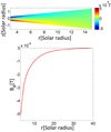Fig. 1. Toroidal magnetic field obtained in the axisymmetric accretion disk model. Upper panel: spatial distribution of the toroidal magnetic field in the disk. Lower panel: magnitude of the toroidal magnetic field at 2° above the midplane as a function of r.

This field is antisymmetric with respect to the midplane of the disk. Its maximum value is about 4 orders of magnitude smaller than B_*, and located at the inner radius of the disk; it decays with radius to almost 80% of its maximum value at r = 10 r_*. To observe these features in more detail, the lower panel in Fig. 1 shows the intensity of the magnetic field at 2° above the disk midplane as a function of r.

The magnitude of the poloidal field can be appreciated in Fig. 2, where the θ component of the magnetic field at the upper surface of the disk is presented as a function of radius. The same figure shows that the radial decay is somewhat slower than that given by the law r⁻¹, with a much slower decay than r⁻³, which is characteristic of a dipolar field.

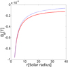Fig. 2. Bθ on the upper surface of the accretion disk. Solid line: field magnitude. Dotted line: fitting using the function $\frac{c}{r}$, with c a constant.

The poloidal magnetic field lines are shown in Fig. 3 as obtained from the Ψ function. In order to present a clearer global view of the magnetic lines, only a few of them are shown and they are not equally spaced in magnitude because the magnetic field magnitude can be better appreciated in the previous figure. Field lines passing through the disk are outwardly bent in angles of less than 60° relative to the disk surface, indicating a section of the disk where mass loss by centrifugal forces is possible (Blandford & Payne 1982). The separation between field lines of the star and the lines of the disk occurs at the disk inner radius. During the evolution of the system, the lines originated in the star that initially threaded the disk are expelled into the magnetosphere. A more detailed view of the lines close to the disk inner radius is shown in Fig. 4, indicating the compression of the field lines between the star and the disk due to the mentioned expulsion of the lines toward the star.

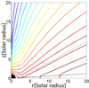Fig. 3. Poloidal magnetic field lines. The central object and the disk are also depicted. The dotted line shows the limiting field line originating in the disk.

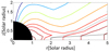Fig. 4. Zoom in on the poloidal magnetic field lines near the central body. The central object and the disk are also depicted. The dotted line shows the limiting field line originating in the disk.

The secondary mass flow generated by the Lorentz force in the disk, in addition to the basic accretion flow, is shown in Fig. 5. Throughout almost the entire length of the disk, the radial component of the velocity of the secondary flow points away from the accretion center, and only near the surface is this flow directed to that center. This secondary mass flow amounts to approximately 10⁸ kg s⁻¹, about 9 orders of magnitude smaller than Ṁ, indicating a very small perturbation to the main accretion flow. However small, this secondary flow is important for the dynamo effect in its contribution to the α effect through the corresponding ${\omega }_s^{(1)}$ in Eq. (10).

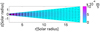Fig. 5. Velocity of the secondary mass flow in the accretion disk. The color of the graph represents the absolute value of the velocity, and the vectors represent the direction of motion.

5.2. Systems with different parameters

We present here some of the results we obtained for a different set of values of M_*, B_*, Ṁ, and r_i. The magnetic field intensity in the disk is strongly dependent on the star magnetic field B_*, and so this parameter was used to distinguish the different cases. In this way, for each of the three values B_* = 10⁻⁶ T, B_* = 10⁻⁴ T, and B_* = 10⁻² T, we tabulate the maximum values of toroidal and zonal magnetic field of the disk according to the different values of Ṁ, r_i , and M_* in Tables 1–3.

Two values of Ṁ were used: Ṁ = 10¹⁷ kg s⁻¹, similar to accretion rates found in the T Tauri systems, and Ṁ = 10²⁰ kg s⁻¹. This parameter has the least influence on the toroidal magnetic field intensity in the disk. As expected from the magnetic field dragging by the mass flow, however, for the largest Ṁ, the magnetic field is more concentrated near the inner radius.

For the stellar mass, values below, similar, and above solar were chosen: M_* = 10²⁷, M_* = 10³⁰, and M_* = 10³³. As expected from the contribution of the dynamo Ω-effect, dependent on the velocity shear, the more strongly affected component is B_ϕ, which increases in magnitude with M_*, while the poloidal component is only slightly affected. A similar effect for B_ϕ should be caused by the increment in velocity shear as the inner radius of the disk is closer to the star. This is indeed seen for the set of values of r_i we chose: r_i = 1.1 r_*, r_i = 2 r_*, and r_i = 10 r_*. However, the change in r_i also has a marked effect on the poloidal component, with variations of up to 50% of its magnitude for the set of inner radii we explored.

6. Discussion

For all parameter sets we studied, the obtained magnetic field configurations are qualitatively similar and are also similar to those in other works, such as Contopoulos et al. (2006), C̆emeljić et al. (2019), Mishra et al. (2020), where diverse approaches to the problem were used. A result worth noting is the decay with radius of B_θ at the disk surface as close to but slower than r⁻¹. This result is similar to that in Latif & Schleicher (2016), where simulations with an α − Ω dynamo show a dependence on r between r⁻¹ and r^−1.5.

The fact that the poloidal field lines tend to accumulate near the internal radius, thus leading to relatively intense magnetic fields, was discussed in Shu et al. (1994). This effect occurs mainly for objects with sizes and magnetic fields similar to those of T Tauri stars. Due also to the dragging of the magnetic field by the mass flow, the effect is further increased when the mass accretion rate increases. Both effects are found in the simulations performed in this work. Moreover, Miller & Stone (1997) presented different magnetic field configurations as a function of the plasma β, which are similar to those in this work in the case of low β, consistent with the Grad–Shafranov description used.

Ghosh & Lamb (1979), Shu et al. (1994), Matt & Pudritz (2005), Lai (2014), and C̆emeljić et al. (2018) determined the radius R_x in the disk that separates stellar field lines from those that originated in the disk. In particular, C̆emeljić et al. (2018) found through MHD simulations with parameters similar to those used here that R_x = 2.9R_*. At variance with this result, the field lines of the star do not cross the disk in all cases considered in our simulations.

C̆emeljić et al. (2018) also found that the poloidal magnetic field magnitude scales almost linearly with that of the star, and that the poloidal magnetic field within the disk is approximately 3 orders of magnitude smaller at a distance of 10 R_*. The almost linear relation between field magnitudes is similar to what was obtained with our model, but with a somewhat slower decay with radius. In addition, the poloidal field is approximately one order of magnitude larger than that obtained in that work.

Finally, we verified that the stationary solutions we presented are independent of the initial conditions considered by starting with initial fields in the disk that are an order of magnitude smaller or larger than those determined by the field of the star. The reason is that the sheared rotation of the Keplerian disk has a strong dynamo effect that rapidly modifies any initial field. In addition, the magnetosphere strongly links the field of the star to that of the disk, so that fixing the field at the stellar surface conditions the possible stationary solutions.

7. Conclusions

We have applied a model for an axisymmetric large-scale magnetic dynamo to an accretion disk, described by the Sakura & Sunyaev model, around a star with a dipolar magnetic field, including a magnetosphere described by the Grad–Shafranov equation. The dynamo model we used has the advantage of being a large-scale model, derived from fundamental MHD equations with a minimum of assumptions, and applied to accretion disks for the first time.

A basic magnetic field configuration was found in which magnetic field lines that originated in the star are concentrated near the internal radius of the disk, always outside the disk. The disk magnetic field has an inclination toward the disk surface that favors centrifugally driven outflows. Moreover, for angles near the rotation axis, the field lines tend to approach the axis, which could favor collimation in case of jets.

We also studied the relation of the disk magnetic field intensity to different parameters of the system such as stellar mass, stellar magnetic field, mass accretion rate, and internal radius of the disk. The results of the magnetic field configuration, magnitude, and the relation to the parameters of the system compare well with those by other authors who used diverse approaches, showing some features that are particular to the dynamo model used, however, such as the relative slow decay with radius of the poloidal field of the disk, and the expulsion from the disk of field lines that originated in the central object.

Acknowledgments

This work was supported by the University of Buenos Aires, grant UBACyT 20020190100198BA. C.P. acknowledges a doctoral fellowship from the University of Buenos Aires.

References

Appendix A: Expressions of the S components

The explicit expression of the term S_ϕ that enters Eq. 2 is

$$\begin{array}{cc}\hfill S_{\varphi }& =\frac{{\lambda }^2}{24r^2}[-B_r{U}_{\theta }-U_r{\partial }_{\theta }{B}_r-U_{\theta }{\partial }_{\theta }{B}_{\theta }+B_r{\partial }_{\theta }{U}_r\hfill \\ \hfill & +{\partial }_{\theta }{B}_{\theta }{\partial }_{\theta }{U}_r-{\partial }_{\theta }{B}_r{\partial }_{\theta }{U}_{\theta }+B_{\theta }(U_r+{\partial }_{\theta }{U}_{\theta })\hfill \\ \hfill & +r^2({\partial }_r{B}_{\theta }{\partial }_r{U}_r-{\partial }_r{B}_r{\partial }_r{U}_{\theta })].\hfill \end{array}$$(A.1)

On the other hand, it is convenient to express the terms depending on S in Eq. 3 by separating them into a part associated with the differential rotation and another part associated with the meridional flow. The part corresponding to the differential rotation is written as

$$\begin{array}{cc}& {(\mathrm{\nabla }\times \mathit{S})}^{\mathrm{\Omega }}·{\mathbf{e}}_{\varphi }=\frac{{\lambda }^2}{24r^2}[F_r{B}_r+F_{\theta }{B}_{\theta }+F_{r\theta }{\partial }_r{B}_{\theta }\hfill \\ \hfill & +F_{\theta r}{\partial }_{\theta }{B}_r+F_{\theta \theta }{\partial }_{\theta }{B}_{\theta }],\hfill \end{array}$$(A.2)

where

$$\begin{array}{cc}\hfill F_r& =3cos\theta {\partial }_{\theta }\mathrm{\Omega }+sin\theta ({\partial }_{\theta \theta }\mathrm{\Omega }+r{\partial }_r\mathrm{\Omega }-2r^2{\partial }_{\mathit{rr}}\mathrm{\Omega }),\hfill \\ \hfill \end{array}$$

$$\begin{array}{cc}\hfill F_{\theta }& =\frac{3+cos2\theta }{2}csc\theta {\partial }_{\theta }\mathrm{\Omega }-rsin\theta {\partial }_{r\theta }\mathrm{\Omega }-r^{2}cos\theta {\partial }_{\mathit{rr}}\mathrm{\Omega },\hfill \\ \hfill F_{r\theta }& =r^{2}sin\theta {\partial }_{r\theta }\mathrm{\Omega },\hfill \\ \hfill F_{\theta r}& =rcos\theta {\partial }_r\mathrm{\Omega }-sin\theta {\partial }_{\theta }\mathrm{\Omega }+rsin\theta {\partial }_{r\theta }\mathrm{\Omega },\hfill \\ \hfill F_{\theta \theta }& =cos\theta {\partial }_{\theta }\mathrm{\Omega }+sin\theta {\partial }_{\theta \theta }\mathrm{\Omega }-r^{2}sin\theta {\partial }_{\mathit{rr}}\mathrm{\Omega }.\hfill \end{array}$$(A.3)

The part associated with the meridional flow is given by

$$\begin{array}{cc}& {(\mathrm{\nabla }\times \mathit{S})}^U·{\mathbf{e}}_{\varphi }=-\frac{{\lambda }^2}{24r^2}[G_r{\partial }_r{B}_{\varphi }+G_{\theta }{\partial }_{\theta }{B}_{\varphi }+G_{r\theta }{\partial }_{r\theta }{B}_{\varphi }\hfill \\ \hfill & +G_{\mathit{rr}}{\partial }_{\mathit{rr}}{B}_{\varphi }+G_{\theta \theta }{\partial }_{\theta \theta }{B}_{\varphi }],\hfill \end{array}$$(A.4)

where

$$\begin{array}{cc}\hfill G_r& =U_r+U_{\theta }cot\theta +r{\partial }_r{U}_r+r^2{\partial }_{\mathit{rr}}{U}_r+r{\partial }_{r\theta }{U}_{\theta },\hfill \\ \hfill G_{\theta }& =(U_{r}cot\theta +U_{\theta }{csc}^2\theta +{\partial }_{\theta \theta }{U}_{\theta })/r-{\partial }_r{U}_{\theta }+{\partial }_{r\theta }{U}_r,\hfill \\ \hfill G_{r\theta }& =-U_{\theta }+{\partial }_{\theta }{U}_r+r{\partial }_r{U}_{\theta },\hfill \\ \hfill G_{\mathit{rr}}& =r^2{\partial }_r{U}_r,\hfill \\ \hfill G_{\theta \theta }& =(U_r+{\partial }_{\theta }{U}_{\theta })/r.\hfill \end{array}$$(A.5)

All Tables

All Figures

	Fig. 1. Toroidal magnetic field obtained in the axisymmetric accretion disk model. Upper panel: spatial distribution of the toroidal magnetic field in the disk. Lower panel: magnitude of the toroidal magnetic field at 2° above the midplane as a function of r.
In the text

	Fig. 2. Bθ on the upper surface of the accretion disk. Solid line: field magnitude. Dotted line: fitting using the function $\frac{c}{r}$, with c a constant.
In the text

	Fig. 3. Poloidal magnetic field lines. The central object and the disk are also depicted. The dotted line shows the limiting field line originating in the disk.
In the text

	Fig. 4. Zoom in on the poloidal magnetic field lines near the central body. The central object and the disk are also depicted. The dotted line shows the limiting field line originating in the disk.
In the text

	Fig. 5. Velocity of the secondary mass flow in the accretion disk. The color of the graph represents the absolute value of the velocity, and the vectors represent the direction of motion.
In the text

References

- Blandford, R. D., & Payne, D. G. 1982, MNRAS, 199, 883 [CrossRef] [Google Scholar]
- Buccino, A. P., Sraibman, L., Olivar, P. M., & Minotti, F. O. 2020, MNRAS, 497, 3968 [NASA ADS] [CrossRef] [Google Scholar]
- Burrows, C. J., Stapelfeldt, K. R., Watson, A. M., et al. 1996, ApJ, 473, 437 [Google Scholar]
- C̆emeljić, M., Kluźniak, W., & Parthasarathy, V. 2019, MNRAS, submitted [arXiv:1907.12592] [Google Scholar]
- C̆emeljić, M., Parthasarathy, V., & Kluźniak, W. 2018, Proc. Int. Astron. Union, 14, 264 [CrossRef] [Google Scholar]
- Contopoulos, I., Kazanas, D., & Christodoulou, D. M. 2006, ApJ, 652, 1451 [NASA ADS] [CrossRef] [Google Scholar]
- Dominik, C. 2015, EPJ Web Conf., 102, 00002 [NASA ADS] [CrossRef] [EDP Sciences] [Google Scholar]
- Dudorov, A. E., & Khaibrakhmanov, S. A. 2016, Astron. Astrophys. Trans., 29, 429 [NASA ADS] [Google Scholar]
- Ghosh, P., & Lamb, F. K. 1979, ApJ, 234, 296 [Google Scholar]
- Hogg, J. D., & Reynolds, C. S. 2018, ApJ, 861, 24 [NASA ADS] [CrossRef] [Google Scholar]
- Kenyon, S. J., Yi, I., & Hartmann, L. 1996, ApJ, 462, 439 [NASA ADS] [CrossRef] [Google Scholar]
- Lai, D. 2014, EPJ Web Conf., 64, 01001 [NASA ADS] [CrossRef] [EDP Sciences] [Google Scholar]
- Latif, M. A., & Schleicher, D. R. 2016, A&A, 585, A151 [NASA ADS] [CrossRef] [EDP Sciences] [Google Scholar]
- Li, J., & Cao, X. 2016, ApJ, 872, 149 [Google Scholar]
- Matt, S., & Pudritz, R. E. 2005, ApJ, 632, L135 [Google Scholar]
- Miller, K. A., & Stone, J. M. 1997, ApJ, 489, 890 [NASA ADS] [CrossRef] [Google Scholar]
- Minotti, F. O. 2000, Phys. Rev. E, 61, 429 [CrossRef] [Google Scholar]
- Mishra, R., C̆emeljić, M., & Kluźniak, W. 2020, ArXiv e-prints [arXiv:2012.13194] [Google Scholar]
- Pope, S. B. 2000, Turbulent Flows (Cambridge: Cambridge University Press), 587 [Google Scholar]
- Scotti, A., Meneveau, C., & Lilly, D. K. 1993, Phys. Fluids A: Fluid Dyn., 5, 2306 [CrossRef] [Google Scholar]
- Shakura, N. I., & Sunyaev, R. A. 1973, A&A, 24, 337 [NASA ADS] [Google Scholar]
- Shu, F., Najita, J., Ostriker, E., et al. 1994, ApJ, 429, 781 [Google Scholar]
- Sraibman, L., & Minotti, F. 2016, MNRAS, 456, 3715 [CrossRef] [Google Scholar]
- Sraibman, L., & Minotti, F. 2019, Sol. Phys., 294, 14 [NASA ADS] [CrossRef] [Google Scholar]
- Stepanovs, D., Fendt, C., & Sheikhnezami, S. 2014, ApJ, 23, 29 [NASA ADS] [CrossRef] [Google Scholar]
- Williams, J. P., & Cieza, L. A. 2011, ARA&A, 49, 67 [Google Scholar]