| Issue |
A&A
Volume 678, October 2023
|
|
|---|---|---|
| Article Number | A66 | |
| Number of page(s) | 15 | |
| Section | The Sun and the Heliosphere | |
| DOI | https://doi.org/10.1051/0004-6361/202346659 | |
| Published online | 05 October 2023 | |
Two-fluid reconnection jets in a gravitationally stratified atmosphere⋆
Centre for mathematical Plasma Astrophysics, KU Leuven, 3001 Leuven, Belgium
e-mail: This email address is being protected from spambots. You need JavaScript enabled to view it.
Received:
14
April
2023
Accepted:
11
July
2023
Abstract
Context. Density decreases exponentially with height in the gravitationally stratified solar atmosphere, and therefore collisional coupling between the ionized plasma and the neutrals also decreases. Reconnection is a process observed at all heights in the solar atmosphere.
Aims. Here, we investigate the role of collisions between ions and neutrals in the reconnection process occurring at various heights in the atmosphere.
Methods. We performed simulations of magnetic reconnection induced by a localized resistivity in a gravitationally stratified atmosphere, in which we varied the height of the initial reconnection X-point. We compared a magnetohydrodynamic (MHD) model and two two-fluid configurations: one in which the collisional coupling was calculated from local plasma parameters, and another in which the coupling was decreased so that collisional effects would be enhanced. The latter setup has a more representative solar collisionality regime.
Results. Simulations in a stratified atmosphere show similar structures in MHD and two-fluid simulations, with strong coupling. However, when collisional effects are increased to attain representative parameter regimes, we find a nonlinear runaway instability, which separates the plasma-neutral densities across the current sheet (CS). With increased collisional effects, the initial decoupling in velocity heats the neutrals and this sets up a nonlinear feedback loop, according to which neutrals migrate outside the CS, replacing charged particles that accumulate toward the center of the CS.
Conclusions. The reconnection rate has a maximum value of around 0.1 for both reconnection heights, and is consistent with the locally enhanced resistivity used in all three models. The early-stage plasmoid formation observed near the end of our simulations is influenced by the outflow from the primary reconnection point, rather than by collisions. We synthesized optically thin emission for both MHD and two-fluid models, which can show a very different evolution when the charged-particle density is used instead of the total density. Our simulations have relevance for observed plasmoid features associated with chromospheric to low-coronal flare events.
Key words: Sun: flares / Sun: magnetic fields / plasmas / methods: numerical / magnetohydrodynamics (MHD)
Movies associated to Figs. 3 and 9 are available at https://www.aanda.org.
© The Authors 2023
 Open Access article, published by EDP Sciences, under the terms of the Creative Commons Attribution License (https://creativecommons.org/licenses/by/4.0), which permits unrestricted use, distribution, and reproduction in any medium, provided the original work is properly cited.
This article is published in open access under the Subscribe to Open model. This email address is being protected from spambots. You need JavaScript enabled to view it. to support open access publication.
1. Introduction
The temperature increases steeply toward the corona of the quiet Sun, throughout the transition region (TR) located at ≈2.5 Mm, and coronal plasma becomes fully ionized (O’Flannagain et al. 2015). Observations have shown that field lines below ≈2.5 Mm can change their connectivity in about 1.5 h, suggesting fast reconnection mechanisms in the solar chromosphere (Close et al. 2004; Yamada et al. 2010).
The reconnection mechanism involved in solar flares releases a huge amount of magnetic energy, and therefore it is believed that reconnection is driven at large scales, evolving toward a Petschek-type configuration (Sato & Hayashi 1979). Petschek (Petschek 1963) proposed a stationary 2D reconnection model that extends a Sweet-Parker (Sweet et al. 1958; Parker 1957) layer (the diffusion region) at the center with standing slow-mode shocks from its ends. The Sweet-Parker reconnection rate scales as ∝S−1/2, where the nondimensional Lundquist number, S, is defined as S = vAL/η, with vA being the Alfvén speed, L a hydrodynamic characteristic length, and η the value of the resistivity (in units of m2 s−1). This classical resistive magnetohydrodynamic (MHD) model proposed by Petschek (1963) predicts much higher reconnection rates than the Sweet-Parker model, where it scales as ∝ln−1(S). For a value of S = 106, the Petschek-type reconnection gives a reconnection rate 65 times larger than the Sweet-Parker model (Leake et al. 2012) does. With greater resistivity, the slow shocks become wider (Sato & Hayashi 1979). The magnetic energy decreases, being converted into thermal energy through Ohmic heating near the diffusion region, and to kinetic energy through the work done by the Lorentz force away from the diffusion region, especially at the location of the slow shocks (Ugai 1995). In simulations of driven reconnection, anomalous resistivity is assumed in order to impede the unbounded growth of the current density (Sato & Hayashi 1979; Ugai 1995; Uzdensky 2003).
Anomalous resistivity can be produced by ion acoustic turbulence, and is then a function of the ion-electron drift velocity, as shown by Manheimer & Flynn (1971). A more simplified but frequently adopted model of anomalous resistivity is one of a space-localized resistivity around the X point, which is also used in this paper. Unlike anomalous resistivity, which depends on the current density, the localized resistivity only depends on space, but both prescriptions lead to fast magnetic reconnection (Biskamp & Schwarz 2001). Although the locally enhanced resistivity leads to fast reconnection, it is not very clear whether the fast reconnection is due to the high value of the local resistivity in the diffusion region or to the localization (Biskamp & Schwarz 2001). Numerical 2D resistive MHD simulations found that having a flat local resistivity profile near the X point can induce spontaneous symmetry breaking in the otherwise symmetric Petschek configuration Baty et al. (2014). In this paper, the up-down symmetry is additionally broken by the gravity and we extend the Petschek reconnection findings to a two-fluid, plasma-neutral setting.
Many simulations have studied the standard solar-flare scenario, in which a vertical current sheet (CS) evolves to form post-flare loops. Takasao et al. (2015) studied post-flare loops in the MHD approximation using a 2.5D setup in which gravity is neglected and thermal conductivity is adopted along the field lines. In their simulations, Petschek-type reconnection develops because of localized resistivity and the slow shocks are essentially isothermal due to effective thermal conductivity. Wang et al. (2021) studied reconnection in a 2.5D MHD setup, using a spatially localized resistivity and an analytic density profile, with uniform pressure. In their model, gravity is neglected, while anisotropic thermal conductivity is incorporated. The reconnection rate is found to be slightly lower when the amount of plasma, β, increases, and the rate is also lower with thermal conductivity. The reconnection rate reaches a maximal value of 0.01. The authors show that reconnection at the termination shock, due to interaction between magnetic islands formed along the primary CS and the magnetic arcade below, is almost as important as reconnection in the main CS for releasing magnetic energy. Jets produced by MHD simulations of Petschek reconnection in a 2D setup without gravity have the properties of small-scale flares observed in the solar atmosphere (Innes & Tóth 1999). State-of-the-art solar-flare simulations extend these efforts with the inclusion of gravitational stratification, and even include the effect of fast electron beams that self-consistently interact with large-scale MHD simulations, identifying many ingredients found in actual observations (Ruan et al. 2020). The step to fully 3D MHD simulations, including gravity, thermal conduction, and reproducing turbulent regions consistent with observed nonthermal velocities, was made in Ruan et al. (2023). Extreme-ultraviolet (EUV) synthetic images produced from these 3D flare models show very good agreement with observations. However, extension to plasma-neutral setups is needed to address more chromospheric-flare counterparts, and this work is a first step toward that goal.
Reconnection jets have been observed at all heights in the solar atmosphere, from the photosphere to the corona (Schmieder et al. 2022), in both cool and hot spectral lines. Takasao et al. (2013) suggest that spicules are chromospheric jets in emerging flux regions, which disappear in chromospheric line images before returning, probably due to heating. Hot and cool jets observed by Schmieder et al. (1995) form, it has been suggested, in the lower corona or upper chromosphere. Aspects of coronal X-ray jets were successfully reproduced in simulations by Yokoyama & Shibata (1996). Chromospheric anemone jets with velocities of 10 km s−1, comparable to the local Alfvén speed, were observed in the upper chromosphere, but could not be observed in the lower chromosphere, where the Alfvén speed is much lower (Takasao et al. 2013).
Many observations show clear signatures of plasmoids that formed during the reconnection process, and their motions are tracked using emission signatures. Plasmoids have been observed as periodic blobs in optically thin Atmospheric Imaging Assembly (AIA) lines (Kumar et al. 2023). These plasmoids can appear in the nonlinear evolution of CSs that are liable to linear resistive-tearing modes. Since plasmoids form on the CSs that also develop Petschek-type configurations with outflows, once they have formed, it is relevant to study the linear stability of a CS in the presence of outflows. In an early, 2D, purely linear MHD analytical study, it was shown that outflows have a stabilizing effect on the tearing mode (Bulanov et al. 1978). In this paper, we discuss stability aspects of a CS due to tearing in a two-fluid setting. Our simulations contain plasmoids, and we make synthetic images that directly relate to the observed blob features.
Since our study uses a plasma-neutral two-fluid model, several works that looked into two-fluid reconnection are of direct relevance to it. Two-dimensional simulations in the two-fluid approach show that the reconnection rate increases because of recombination and larger outflows (Leake et al. 2012). Ionization or recombination processes would put additional constraints on the background stratification, leading to nontrivial equilibrium conditions (Snow & Hillier 2021). A non-static equilibrium introduces a new free parameter through the gradient in the vertical velocity, and can moreover explain the formation and properties of the TR (Song et al. 2023). In this paper, we generalize the work to stratified settings, but do not include ionization or recombination processes in our simulations. Leake et al. (2013) obtain high reconnection rates of around 0.1 due to two-fluid effects, which otherwise would be obtained by using the Hall effect, kinetic effects, or localized resistivity. In stratified setups that were liable to the Rayleigh-Taylor instability, secondary reconnection events showed that two-fluid effects are locally very important (Popescu Braileanu et al. 2023). Murtas et al. (2021) find that plasmoid coalescence happens faster in the two-fluid model than in MHD, because the effective Alfvén speed, based on a two-fluid density defined by the collisional coupling, is larger. In 1D two-fluid simulations of slow magneto-acoustic shocks (of the type relevant in a Petschek-type reconnection region), frictional heating leads to a localized region around the “reconnection” point with an increased temperature in the neutral fluid Hillier et al. (2016). As a consequence, a blast wave in the neutral fluid develops, with overshoots in the neutral density and velocity (Hillier et al. 2016; Snow & Hillier 2019). We show in our multidimensional setup how the detailed CS structure may show intricate decoupling (and runaway) effects in the Petschek-type configuration. Here, we extend previous work by studying reconnection in a 2D stratified setup, accounting for the presence of coupled plasma-neutral species.
We present the numerical setup in Sect. 2 and the results of our simulations in Sect. 3. We created synthetic views from the simulation snapshots, which we present in Sect. 4. We summarize our conclusions in Sect. 5.
2. Numerical setup
We consider a gravitationally stratified atmosphere in which we defined a temperature profile with height z, described by
![Mathematical equation: $$ \begin{aligned} T(z)=T_{\rm ch} + \frac{T_{\rm co}-T_{\rm ch}}{2}\left[\text{ tanh}\left( \frac{z-z_{\rm tr}}{{ w}_{\rm tr}} \right) +1\right]\,, \end{aligned} $$](/articles/aa/full_html/2023/10/aa46659-23/aa46659-23-eq1.gif) (1)
(1)
in which wtr = 0.2 Mm, the TR height is ztr = 2 Mm, and the chromospheric and coronal temperatures were set through Tch = 8 × 10³ K and Tco = 1.8 × 10⁶ K, respectively. The initial profiles of the temperature, and of the neutrals and charges, as well as total fluid densities, are shown in Fig. 1. We used an ideal equation of state for both neutrals and charges, and the normalized mean molecular weight was considered uniform and constant, having the values of 0.5 for charges and 1 for neutral species (Popescu Braileanu & Keppens 2022).
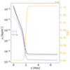 |
Fig. 1. Initial profiles as a function of height. For the densities, neutrals (dashed blue line), charges (dotted red line), and the total (solid black line) are on the left axis. The temperature (solid orange line) is on the right axis. |
We used a force-free sheared magnetic field, changing its far-field (large horizontal coordinate |x|) vertical orientation near x = 0, with uniform magnitude B0 = 10−3T, given by
 (2)
(2)
in which Ls = 0.02 Mm. A similar force-free profile was used in the simulations of Ruan et al. (2020, 2023). The CS width, calculated as the full width at half maximum (FWHM) of the corresponding current density component, Jy0, is 0.036 Mm.
We used a localized resistivity of the particular form
 (3)
(3)
in which η0 ≈ 8 Ωm and η1 ≈ 0.8 Ωm. The reconnection point is always at x = 0, but we varied the reconnection height, zrec, as mentioned in Sect. 2.2, below. To trigger the reconnection, we adopted an initial velocity variation. We only allowed the initial perturbation to go in the x direction, in an attempt to bring the field lines closer around the reconnection point, which has the form
 (4)
(4)
with
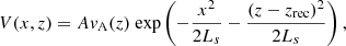 (5)
(5)
and
 (6)
(6)
the total Alfvén speed, with ρtot = ρn + ρc the total density. We chose the amplitude A = 10−1. In a two-fluid simulation, this initial perturbation is the same for the velocity of charges and neutrals.
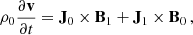
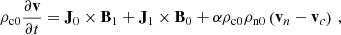
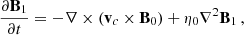
The two-fluid model uses the newly developed module in the fully open-source MPI-AMRVAC code (Popescu Braileanu & Keppens 2022; Keppens et al. 2023). The equations solved are the nonlinear, compressible, resistive two-fluid Eqs. (1)–(7) from Popescu Braileanu & Keppens (2022). In a 2.5D geometry, the domain xz with x ∈ [ − 0.5, 0.5] Mm and z ∈ [0, 7] Mm is covered by a grid with a base resolution of 256 × 1024, and we used five levels of refinement, resulting in an effective resolution of 1024 × 4096 points and the size of the finest cell Δx = 9.76 × 10⁻⁴ Mm and Δz = 1.7 × 10⁻³ Mm. The bottom boundary in the z direction was closed (antisymmetric for vertical velocities and symmetric for the rest of the variables), and we used open boundary conditions (symmetric for all the variables) for the top boundary and both side boundaries in the x direction. The region −0.2 ≤ x ≤ 0.2 was always refined at the highest level, so that the CS was properly resolved. The refinement criterion is based on density only for the MHD cases and equally on charged and neutral density in the two-fluid runs. We used the splitting of the equilibrium force-free magnetic field (Xia et al. 2018) and the gravity stratification for both neutrals and charges (Yadav et al. 2022; Popescu Braileanu & Keppens 2022). Under this approach, the magnetic field, B, densities, ρn and ρc, and pressures, pn and pc, were split into time-independent, B0, ρn0, ρc0, pn0, and pc0, and time-dependent, B1, ρn1, ρc1, pn1, and pc1, parts. The equations solved in the code are for time-dependent quantities, while the equilibrium conditions were explicitly removed from the equations:
 (7)
(7)
Mathematically, the split equations are equivalent to the unsplit equations, but, numerically, splitting helps to avoid an unwanted evolution due to the numerical dissipation of the equilibrium.
2.1. Coupling aspects
Because of the very low mass of electrons compared to ions, the collisions between charges and neutrals are effectively collisions between ions and neutrals, and the mean-free path between ions and neutrals and between neutrals and ions can be defined as
 (8)
(8)
in which νin = αρn and νni = αρc denote collision frequencies between ions and neutrals and between neutrals and ions, respectively (see Eq. (15) in Popescu Braileanu & Keppens 2022). The characteristic velocity is the Alfvén speed of the whole fluid, as defined (generalized to vA(x, z, ;t)) by Eq. (6), (see also Eq. (37) in Popescu Braileanu & Keppens 2022, in which the characteristic velocity was chosen as the fast magneto-acoustic speed). The collisional parameter, α, (see Eq. (A.3) in Popescu Braileanu & Keppens 2022) is defined as
 (9)
(9)
in which the collisional cross section considered here is Σin = 10−19 m2, and Tcn is the average of the temperatures of the neutrals and charges. In this paper, we consider two cases for the collisional coupling: one in which α(x, z; t) is calculated consistently from instantaneous plasma parameters; and another in which it is set to a constant value. When α is calculated self-consistently, its profile varies slowly with height, with values initially between 5.8 × 10¹² m3 kg−1 s−1 and 8.2 × 10¹² m3 kg−1 s−1. These minimum and maximum values remain practically unchanged at the end of the simulation. The high values imply that the coupling is near perfect (hence MHD-like behavior is expected) throughout the domain. We compared this to a run in which we instead set α to a constant value throughout. This constant value of α = 3.84 × 10⁸ m3 kg−1 s−1 is almost four orders of magnitude smaller than the consistently computed values. However, as we argue in the section below, this reduced coupling value ends up being more representative for actual solar settings. Moreover, in that regime, we have two-fluid effects that are important in stratified reconnection setups.
2.2. Parameters of the simulations
For our study of reconnection in stratified settings, we compared three collisional regimes, namely: (i), a single fluid MHD model (label “MHD”); (ii), a two-fluid plasma-neutral model in which the collisional parameter, α, is calculated self-consistently from plasma values (label “2fl”); and (iii), a two-fluid model in which the collisional parameter α is constant and set to a smaller value of 3.84 × 10⁸ m3 kg−1 s−1 (label “2flα”). We studied six cases in total, since for each collisional regime the reconnection point varies, from zrec = 2 Mm for reconnection in the upper chromosphere to the low TR, to zrec = 4.5 Mm for coronal reconnection.
In the MHD model, the initial equilibrium atmosphere was constructed by summing the densities (shown in Fig. 1) and pressures for charged and neutral fluid at all heights. The resulting mean-free paths between ions and neutrals and between neutrals and ions for the two two-fluid models, 2fl and 2flα, are shown in Fig. 2. In this 2flα case, both values of the mean-free path in the TR and above are 𝒪(0.01 Mm), and hence they are similar to the width of the CS, while in the 2fl case the values of the mean-free path are 𝒪(10−6 Mm). Because of the weak dependence on height of the value of α calculated self-consistently, both profiles of the mean-free paths (2fl and 2flα) look similar, being dominated by a variation in density, included in the calculation of the mean-free path as from Eq. (8). The mean-free path does not change significantly during the simulation, being determined rather by the equilibrium plasma parameters.
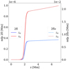 |
Fig. 2. Collisional mean-free paths as functions of height. We show the mean-free paths between ions and neutrals (λin, red lines) and between neutrals and ions (λni, blue lines) for the two collisionality regimes considered: self-consistent from plasma-neutral parameters (2fl, solid lines, left axis) and reduced-case 2flα (dashed and dotted lines, right axis, with a different order of magnitude). The collisional mean-free paths were calculated according to Eq. (8). |
We now argue that the 2flα case is more solar-relevant. Indeed, we used a temperature profile defined by Eq. (1), which is slightly smoother than the Vernazza-Avrett-Loeser (VAL-C) model (Vernazza et al. 1981), but which has the advantage of permitting us to directly control the width (wtr) of the TR. A similar temperature profile defined by an analytic function has been used by other authors (Dover et al. 2021). This overly smooth temperature variation also implies a larger fraction of neutrals at both used reconnection heights, especially at the coronal reconnection point zrec = 4.5 Mm, taking into account that the scale height of the neutrals is half that of the charged particles. The other reconnection case has zrec = 2 Mm; in other words, it starts its reconnection at the middle of the TR. The effectiveness of collisional coupling between plasma-neutral species at these heights is largely set by the densities they attain there.
When we integrated the vertical profiles, at the base of the atmosphere at z = 0, we used the total number density from the VALC model, namely nT ≈ 1023 m−3, but we had to consider an ionization fraction of 0.1, in order to still obtain more charges in the corona despite the smoothing of the temperature profile. Hence, the adopted temperature variation, together with the imposed bottom densities, led to a reversal in the dominance of neutrals over charges at z = 1 Mm, while the entire TR and corona is charge dominated. We find that the overly smoothed temperature profile actually increased the density in the upper chromosphere and corona above observed values, making collisional coupling more significant there. This justifies the use of a smaller and more representative value of α in the simulation 2flα, which mimics the actual coupling found for the normally lower densities. Indeed, the mean-free path between ions and neutrals in the two-fluid reconnection simulations of Leake et al. (2013), which was self-consistently calculated, is about 100 m. This is nicely situated between our 2fl and 2flα case. Moreover, there are different recipes for calculating collisional frequencies, due to the different values for the collisional cross sections available in the literature, which lead to large differences (Martínez-Sykora et al. 2017). The very small mean-free path in our 2fl case suggests that it can be considered an MHD limit case, and this is confirmed in our simulations below.
3. Results
In all six cases considered (examining coronal and TR reconnection for each of the three models: MHD, 2fl, and 2flα), the reconnection develops, producing bidirectional outflow jets and traveling away from the reconnection point. This can be seen in the snapshots of the total density shown in Fig. 3. As the atmosphere is gravitationally stratified, the jets traveling upward are denser and those traveling downward are less dense than the surrounding fluid located at the same height. The figure shows that for TR reconnection, we get a pronounced upward jet that is accompanied by a vertically oriented CS that lengthens as time progresses. From the time evolution of the upward-moving jets in the zrec = 2 Mm case, we can estimate a vertical velocity of ≈8 km s−1. An online animation for this case (z2.0-2flaplha.mp4) overplots the adaptive grid for the neutral density. In the case of coronal reconnection, we find a clear two-sided (up-down) jet forming, in which the lower one ultimately interacts with the TR and chromosphere (forming post-flare loops). For both reconnection heights considered, zrec = 2 Mm and zrec = 4.5 Mm, the MHD (top row) and the 2fl models (middle row) give very similar results, as expected according to the collisionality regime. A clear difference appears in the snapshots for the 2flα model (bottom row of Fig. 3), with the development of a less dense region with an edge of increased density, and this is seen in both zrec cases. In order to better understand these differences, we further analyzed snapshots for zrec = 2 Mm at t = 622.6 s, the last time shown in Fig. 3 (left column).
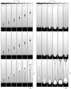 |
Fig. 3. Time evolution of the total density for all six simulations. Left panels: zrec = 2 Mm. Right panels: zrec = 4.5 Mm. A different physics model is shown in each row: MHD (top row), 2fl (middle row), and 2flα (bottom row). An online animation (case z2.0-2flalpha.mp4 or 2flα) overplots the adaptive grid for the neutral density. |
3.1. Analysis of TR reconnection
We plot in Fig. 4 the out-of-plane current density, Jy, for the 2fl and 2flα models, and overplot magnetic field lines and isocontours of total density. Except for the fact that the 2flα seems a bit further evolved in time (as the top magnetic island is located a bit higher), the current-density structures are very similar for the two models. We observe that the dense edges in the 2flα case are located just outside the CSs. Because of the localized resistivity, the simulations evolve toward a Petschek-like reconnection. Slow shocks that accompany the reconnection, traveling in the x direction, gradually widen the distance over which Bz ≈ 0, splitting the CS into two CSs, seen as “V” structures in the images. Theoretically, in an assumed MHD, stationary Petschek reconnection state (without stratification), the slow-shock discontinuity is located along this V pattern, Bz is exactly zero inside the V, and Bx is uniform within. Hence, the two CSs should actually be infinitely thin in the ideal MHD limit that holds away from the resistive reconnection layer. However, in our more realistic setup, we find that it is possible for Bz to locally reverse its sign, creating another CS with Jy of the opposite sign, as is seen most clearly in the snapshot for the 2flα case at height z ≈ 5 Mm, at the location of the corresponding ripple in the magnetic field line. This reversal in the sign of Bz was in 1D two-fluid models associated with a reversal in the sign of vx and was found to be related to the heating produced by the two-fluid effects (Hillier et al. 2016; Snow & Hillier 2019). However, the reversal in the sign of Bz is observed in our MHD (and 2fl) simulations as well, so Ohmic heating might be the cause in our simulations. We note that the magnetic field lines in Fig. 4 show the expected post-flare loop configuration below the reconnection site. The 2flα case also shows a plasmoid structure forming at a later stage; we discuss this in Sect. 3.4.
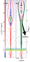 |
Fig. 4. Comparison between the out-of-plane current density. For two-fluid models: 2fl (left) and 2flα (right) at t = 622.6 s. Black lines with arrows are magnetic field lines. Yellow-to-green colored contours relate to the density variation. The ripple in the magnetic field, associated with the reversal in the Bz sign, located at z ≈ 5 Mm, is indicated in the figure. |
We compare snapshots of the density of charges and neutrals in the two models in Fig. 5 (Fig. 3 shows total densities). We observe that, in the 2fl case, the densities of charges and neutrals have similar structures, the difference being mainly in magnitude. The magnitude scales with the background density, with the neutral density being lower in the corona than the charged density. The neutral density shows more variation with height, since the scale height of the neutrals is half that of the charges. In contrast, in the 2flα case, we observe a clear reversal in contrast, namely a central region with low neutral density and high charged density, surrounded by a shell of high neutral density and low charged density. We also show in the charged-density plots the density snapshot of an MHD run in which we used the charged-fluid properties only; this corresponds to the zero-collision, α = 0, limit. The snapshot seems more evolved in time than the previous cases, 2fl and 2flα. A smaller (effective) density implies a higher Alfvén speed and shorter hydrodynamic timescales; however, the edge of increased neutrals is rather related to an incomplete coupling regime, and not to a smaller effective density. Similarly to the conclusion of Murtas et al. (2021), a smaller effective density due to the collisions is associated with shorter timescales and faster evolution, as we have seen previously in Fig. 4. The same reversal can be seen in the temperature maps as well for the 2flα case, as shown in Fig. 6, in which the higher density regions have lower temperatures for both neutrals and charged fluids. The 2fl case (top panels of Fig. 6), however, shows similar structures in the temperatures of neutrals and charges.
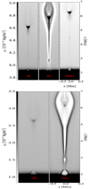 |
Fig. 5. Comparison between the charged densities (top panels) and the neutral densities (bottom panels) for t = 622.6 s. Top row: 2fl (left panel), 2flα (middle panel), and MHD with charged fluid only (right panel). Bottom row: 2fl (left panel) and 2flα (right panel). |
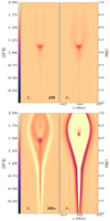 |
Fig. 6. Comparison between the temperatures of neutrals and charges at t = 622.6 s. Top panels: 2f. Bottom panels: 2flα. |
In order to understand this clear difference in the 2flα case, which must be caused by two-fluid effects, we plot in Fig. 7 different quantities along a horizontal cut located at z = 4 Mm. These 1D profiles are consistent with the previous 2D images, most notably Figs. 5 and 6, in which they cut across the V-shaped CS structures discussed earlier. For the 2fl model, the structures in the charged and neutral densities (panels a and b) are similar. The x-velocity (panel c) and temperature (panel d) profiles overlap for both fluids, meaning that the two fluids are coupled in both velocity and temperature. For the 2flα model, more charges imply fewer neutrals and a higher density implies a lower temperature. The temperature of the neutrals increases by more than 1.6 × 10⁶ K at the center of the CS. Further from the center of the CS, the velocities of charges and neutrals are coupled; however, inside the CS they are completely different. The neutral velocity changes sign at the center of the CS, meaning that the neutrals are going out of the CS. Hence, the 2flα case, which shows a pronounced anticorrelated structure in density and temperature for charges versus neutrals, clearly demonstrates decoupling between both species through the CS structure.
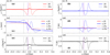 |
Fig. 7. Horizontal cut at coronal height z = 4 Mm at time t = 622.6 s for the simulations with TR reconnection or zrec = 2 Mm. (a) Density of charges. (b) Density of neutrals. (c) x velocity for charges and neutrals. (d) Temperature of charges and neutrals. (e) Total density. (f) Center of mass temperature from Eq. (10). Different curves are for the two models considered – 2fl and 2flα – quantities for charges and neutrals are shown in the same plot in panels c and d, as indicated in the legend. The primary and secondary maximum peaks in the neutral collisional heating term for case 2flα, as shown in detail in Fig. 8 and located at z = −0.03 Mm and z = −0.1 Mm, are indicated by vertical violet and dotted gray lines, respectively. |
Panels e and f in Fig. 7 show the total density, ρ, and the temperature of the center of mass, defined as
 (10)
(10)
The total density profile is very similar to the separate neutral and charged density profile for the 2fl model. In this case, the positive peak in the density and the corresponding negative peak in the temperature are related to the fact that the (vertically flowing) reconnection outflow comes from a lower height with a higher density and a lower temperature. However, the two-fluid solution in the 2flα case, in which the collisional effects are enhanced, behaves rather differently and demonstrates a nonlinear runaway effect. In the case of the 2flα model, there is a central depletion in total density, where charges accumulate and neutrals deplete, and this is surrounded by a layer of enhanced total density, where charges deplete and neutrals accumulate. A tiny positive peak, similar in magnitude to that in the 2fl model, still remains at the very center of the CS. Seen from an MHD point of view, the whole fluid (both neutrals and charges) heats because of the collisions. This creates a peak in the center of mass temperature (panel (f), dotted line) and the entire fluid expands, so that the total density decreases toward the center of the CS (panel (e), dotted line). In the various panels of Fig. 7, vertical dotted lines show extremal positions in the neutral collisional heating term for case 2flα, which are discussed in more detail in what follows.
In order to better understand the temperature and velocity profiles seen in Fig. 7, we show the terms that enter the temperature (top panel) and velocity (bottom panel) equations in Fig. 8. The primary and secondary maximum peaks in the neutral frictional heating term (dashed blue line) for the 2flα case (top-right panel) are located at a distance of 0.03 Mm and 0.1 Mm away from the center of the CS, respectively. The peak in the Ohmic heating term (solid red line) is located close to the primary maximum peak in the neutral frictional heating term of the 2flα case (i.e., near the vertical dotted violet line). This frictional heating is negligible in the 2fl case (top-left panel). In the 2flα case (top-right panel), the charged-fluid frictional heating term (dashed red line) has a similar profile to the neutral frictional heating term but has smaller values because of the higher charged density compared to the neutral density. In the 2flα case, the neutral frictional heating peak value is five times higher than the peak one in the Ohmic heating.
 |
Fig. 8. Horizontal cuts along z = 4 Mm for the case with TR reconnection, or zrec = 2 Mm at time t = 622.6 s, the same time as for Fig. 7. Quantities corresponding to charged and neutral fluid are shown with red lines and blue lines, respectively. Left panels: 2fl case. Right panels: 2flα case. Top row: Terms in the temperature equation; the Ohmic term (solid red line) and collisional heating terms (dashed lines: red for charges and blue for neutrals). Bottom row: Terms in the velocity equation; acceleration is due to magnetic pressure (dashed red line), the gas-pressure gradient (solid lines; red for charges and blue for neutrals), and collisions (dotted lines; red for charges and blue for neutrals). The primary and secondary maximum peaks in the collisional heating associated with neutrals, located (and shown only for negative x, because of symmetry) at z = −0.03 Mm and z = −0.1 Mm, are indicated by vertical dotted violet and gray lines, respectively, for the 2flα case (right panels). |
We now turn our attention to what causes the velocity decoupling effects, by discussing the forces shown in the bottom panels of Fig. 8. The inflow into the CS (as seen in panel c of Fig. 7) is driven by the magnetic pressure gradient, which acts only on charges, producing initial decoupling in the velocities between neutrals and charges when entering the CS. This magnetic pressure gradient pushes the charges and the collisionally coupled neutrals inside the CS against the gradient of their pressures. In the 2fl case, only Ohmic heating matters, and the overall decoupling between neutrals and charges stays minimal throughout the CS. In the 2flα case, the neutral and charged fluids decouple in velocity in a more pronounced way throughout the entire CS, again indirectly driven by the magnetic forces that drive the reconnection. But the initial decoupling grows, and collisional heating of neutrals causes the neutrals to heat, expand, and go out of the CS, accumulating between the primary and secondary heating points (violet and gray lines, respectively), as observed in panel b of Fig. 7. The inflow of charges there decreases because of the increased collisions with the neutrals that accumulated outside the CS (see the local minimum observed for the dotted red curve at the location of the gray line in panel (c) of Fig. 7). The decoupling in velocity therefore increases further, as does the frictional heating at this secondary neutral heating maximum point (the vertical gray line), which again increases the neutral pressure. Thus, the neutral inflow increases as a local maximum is observed for the dotted blue curve at the location of the gray line in panel c of Fig. 7. This is because of the neutral pressure gradient, which shows a local maximum peak in the solid blue curve at the location of the gray line in the bottom-right panel of Fig. 8. This in turn drags the charges into the CS; a local maximum peak is seen for the dotted red line in the bottom-right panel of Fig. 8, which has positive values around the gray line. This implies acceleration of the plasma toward the center of the CS, in the same direction as, and partially overlapping with, the magnetic-pressure gradient curve. Therefore, the velocity of charges toward the center of the CS is increased and has the opposite sign to that of the neutrals, leading to more decoupling and to a runaway, nonlinear instability. The heating of the charges at the primary heating point (violet line) slows down in this runaway instability process. The charges enter faster into the CS because of decreasing collisions with neutrals, and this accelerates the process (in addition to leading to a thinner CS and faster outflows). The runaway process is further enhanced by the charges expanding due to the (collisional) heating at the secondary point (gray line). The runaway process creates a region of accumulating neutrals bordering the CS (within the hydrodynamic timescale on which the charges enter the CS due to the magnetic pressure gradient), which creates a secondary (collisional) heating point whereby the charges get pushed faster into the CS.
3.2. Analysis of coronal reconnection
We next study the case zrec = 4.5 Mm, in which the reconnection was triggered in the coronal region. A zoomed view shown in Fig. 9 shows what happens near and above the TR, after the downward reconnection outflow hits the dense material in the chromosphere and is reflected. The snapshots of the density of neutrals versus charges (top row) show again a pattern of evacuated versus enhanced regions with dense versus evacuated edges. The decoupling in velocity (bottom-left panel of Fig. 9) points across the magnetic field lines and the isocontours of the decoupling in temperature (Tc − Tn), shown in the bottom-right panel, and follows the structures in current density, suggesting that the decoupling is related to the magnetic fields. Smaller CSs are formed at different locations and with different orientations, meaning that this separation of neutral and charged densities across the CS is generally related to reconnection and not determined by gravity or localized resistivity. In a time evolution (an online animation z4.5-2flalpha.mp4 is provided), we see that the process of separation seems to reverse in this case, when the structure rises again, but this is influenced by mixing with both neutral and charged material coming from below. Hence, in both 2flα cases, we find clear evidence of a nonlinear runaway process that enhances the spatial separation between charged and neutral fluids near CSs. This runaway process is clearly related to having a large collisional free path, as compared to the width of the CS, as it is not seen at all in the 2fl model.
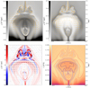 |
Fig. 9. Two-fluid coronal-reconnection downflows impacting the chromosphere. We provide snapshots of charged density (top left), neutral density (top right), out-of-plane current density (bottom left), and charged temperature (bottom right) for the simulation zrec = 4.5 Mm, with 2flα at t = 591.5 s; the last time shown is in the right column at the bottom of Fig. 3. In the panels of neutral and charged densities (top panels), the orange arrows show the velocities of neutral and charged fluid, respectively. We overplot the magnetic field lines and the decoupling velocities over the current density map (bottom-left panel) and isocontours of the temperature decoupling (Tc − Tn) in the range −1.8 × 10⁶ K and 1.8 × 10⁶ K over the charged temperature image (bottom-right panel). |
Overall, we identified a runaway (decoupling) instability in a weakly collisional regime, which occurs in a non-stationary two-fluid setup to the reconnection problem. This ultimately breaks down the fluid assumptions if neutral and charged densities decrease toward zero in separate locations. The exact conditions for the onset of this nonlinear instability, such as the α-collisional parameter range, can be the subject of a more idealized setup (without gravity) in the future.
3.3. Reconnection rate
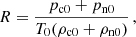
We then calculated the reconnection rate
 (11)
(11)
in the same way as Leake et al. (2013), Murtas et al. (2021). The superscripts indicate the points where quantities are evaluated. The reconnection point, X, is defined as the point where the dissipation,  , is maximum (we included η in this calculation because of the localized resistivity). We note that X is located at the center of the CS (x = 0) at a certain height, which might not be the initial reconnection point, zrec, because this reconnection point migrates vertically, especially in the TR reconnection case zrec = 2 Mm, in which the stratification is stronger. Initially, the X point is located at the height z = zrec, which is one of the parameters of the simulations. The border of the CS, indicated by the superscript up, is defined as the point located at the same height as X but displaced along the x direction, as it is located at the point where the current density is half the current density measured at X. Because of the horizontal symmetry, the values calculated at the two opposing symmetric points at the borders of the CS were averaged, because numerically exact left-right symmetry might not be preserved. The Alfvén velocity,
  , was calculated using the total density evaluated at the reconnection point, X, and the magnetic field,
  . We plot the thusly computed reconnection rate as a function of time in Fig. 10, for both TR and coronal reconnection, each time comparing the MHD rate and both two-fluid rates. The reconnection rate has an initial increase, which is steeper for zrec = 4.5 Mm than for zrec = 2.0 Mm. This is because at zrec = 4.5 Mm the density is lower and the CS thins faster; however, the minimum width of the CS achieved during the simulations is similar for both heights. The maximum reconnection rate reached after this increase phase is M ≈ 0.1, a typical value for reconnection scenarios that use localized resistivity. Then, it decreases for both cases, mainly because the magnetic field dissipates. The reconnection rate decreases much faster in the TR reconnection case that started at zrec = 2.0 Mm, because of the quick and continuous upward migration of the X point over a distance of ≈0.5 Mm at the end of the simulation. It is seen that the reconnection rates remain similar for the MHD and the two two-fluid setups. It is known that the plasmoid formation increases the reconnection rate (Leake et al. 2012; Murtas et al. 2021); however, in our case, the plasmoids appear too late in the simulations to significantly influence the growth rate.
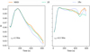 |
Fig. 10. Reconnection rates for the six simulations as a function of time. The two cases of reconnection height are considered: zrec = 2 Mm (left panel) and zrec = 4.5 Mm (right panel). Different curves indicate different models: MHD (solid orange line), 2fl (dashed green line), and 2flα (dotted blue line). |
3.4. Secondary plasmoids
In the last snapshots of the simulations with TR reconnection (zrec = 2 Mm), we can observe the formation of secondary plasmoids, but this is not so in the coronal case (zrec = 4.5 Mm). The plasmoids’ shape can be clearly seen in the current-density map in Fig. 4 for the 2flα case, where we can visually estimate a size of ≈0.3 Mm. The initial formation phase of the plasmoids can be seen best in the vertical profile of the vertical velocity. Several equidistant moments in time are shown in Fig. 11 for the three models: 2flα, 2fl, and MHD. In these profiles, the plasmoids are seen as secondary velocity extrema that develop and get advected upward. The plasmoids move with the outflow from the primary reconnection points, which are at the locations where the vertical velocity changes sign (fitted locally by a linear slope in the three panels). We can visually estimate that the fastest-growing length scales are similar in the three cases; however, the growth is largest in the MHD case, followed by 2flα and then 2fl. This suggests that the two-fluid effects do not affect the initial phase of the growth of these plasmoids. We do expect the later stages of this plasmoid evolution to be similarly affected by the runaway decoupling process in the 2flα case, when charges accumulate toward the middle of the CS.
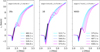 |
Fig. 11. Vertical profiles of the vertical velocity when the plasmoids form for zrec = 2 Mm. Shown for five moments in time in the late stage of the simulations, for the three models: 2flα (left panel), 2fl (middle panel), and MHD (right panel). For the two-fluid models (left and middle panels), we show the velocity of charges. The linear fit of the velocity profile around the reconnection point (where the velocity changes sign) is shown by a black line and the value of the slope is indicated at the top of each panel. |
The linear growth of the tearing mode is affected by the gradient in the vertical flow (parallel to the CS), as shown in a linear resistive MHD analysis about a 2D configuration by Bulanov et al. (1978). In their analysis, the vertical profile is assumed to be linear, vz(z) = az, in which a quantifies the vertical velocity variation. Bulanov et al. (1978) showed that the growth rate, γ(a), of the tearing mode at a finite a is reduced from the case without a flow gradient, a = 0, in the sense that γ(a)≈γ(0)−a.
A linear analysis of the tearing mode in the two-fluid approach, using simplified assumptions of uniform density, and hence no gravity (and no added vertical flow), is presented in Appendix A. This shows that two-fluid effects define an effective density, ρc0 ≤ ρeff ≤ ρT0, between the background charged, ρc0, and total, ρT0, densities. The linear growth of the tearing mode in this simplified two-fluid assumption is bounded between the growth calculated in the MHD assumption when the density is the total density (ρT0) and the charged density (ρc0). In our setup the ionization fraction is high, and the difference that the two-fluid effects might introduce into the growth of the tearing mode is on the order of 10−4 s−1. This is shown in our appendix, and can be seen as the difference on the y-axis of Fig. A.1 between the orange point, which corresponds to the collisional parameter used in 2flα simulations, and the red point, which corresponds to a value of the collisional parameter larger than the maximum value of α in 2fl cases. This two-fluid related difference is one order of magnitude smaller than the obtained difference in the velocity slope, which we show for the three cases in Fig. 11. The ordering of the growth rates of the plasmoids, as visually estimated from Fig. 11, is reversed compared to the ordering of these slopes. This is consistent with the expected reduction in tearing growth rates due to added vertical velocity gradients. Similarly, the large (vertical) gradients in the outflow velocities are probably the reason why we do not observe secondary plasmoids in the simulations with zrec = 4.5 Mm, since then the vertical velocities and corresponding vertical gradients are larger than for the zrec = 2 Mm case. Therefore, in our simulations, the initial linear growth of the plasmoids is instead influenced by the fact that they form at different moments and at slightly different heights during the simulations, when the vertical gradients in the velocity are different. The difference in the growth rate produced by this gradient in velocity is much larger than the difference in the growth rate introduced by the collisional effects.
4. Synthetic views
As a relatively straightforward observational validation, we can produce synthetic images resulting from emission from optically thin spectral lines. To do so, we calculated the emission in the Solar Dynamics Observatory Atmospheric Imaging Assembly (SDO/AIA) channel AIA 193 Å, which has its highest response for temperatures between 106 and 2 × 10⁶ K. We did so only above the height z ≈ 2 Mm in our initially stratified atmosphere, because the chromospheric region itself is not appropriately dealt with in an optically thin limit. It being optically thin emission, we essentially dealt with a function of local temperature, T, and number density, n, given by
 (12)
(12)
in which R(T) is a response function that depends on temperature. A log R − log T view is shown in Fig. 12 for the wavelength 193 Å, obtained using the CHIANTI atomic database (Del Zanna et al. 2015). Images in these EUV channels of AIA can be synthesized from 3D data cubes by integrating Eq. (12) along the line of sight. We have 2.5D data, with an assumed invariance in the third (y) direction. As we have 2.5 D simulations, the images are shown at the simulation resolution, and there is no integration along the line of sight, which has the added effect of rendering units meaningless. As the AIA 193 channel is emitted by Fe XII, emission is obviously from charged species. From our two-fluid plasma-neutral model, we must choose which number density and temperature is taken in Eq. (12). A more accurate result might be obtained by using only the charged density instead of the total density.
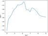 |
Fig. 12. AIA 193 Å response function R(T) as a function of temperature (measured in K), (Del Zanna et al. 2015). Both axes are logarithmic. |
In particular, plasmoids are usually observed as bright blobs due to their increased density compared to the surrounding medium. In this case, models that consider the total density in the calculation of the synthetic image (as is usually done from a single-fluid MHD simulation), as opposed to those that consider the charged-particle density, would give the wrong results. Fig. 13 shows synthetic images in the AIA 193 channel that capture the temporal evolution of the plasmoids. We found secondary plasmoids when zrec = 2 Mm, and show synthetic views for the 2fl case (top row) and the 2flα case (middle row), in which we use the charged-fluid temperature and density, meaning Λ(nc, Tc) in Eq. (12). The bottom row shows the same snapshots for case 2flα as the middle row but instead uses the total density and the center of mass temperature defined by Eq. (10), in practice using Λ(nT, T2fl) in Eq. (12).
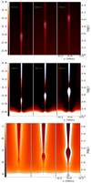 |
Fig. 13. Synthetic views on secondary plasmoids, at three consecutive times. For plasmoids in the case zrec = 2 Mm, we show synthetic images of AIA 193 Å emission. Top row: 2fl case. Middle and bottom rows: 2flα case. For the calculation of emission, we used the density and temperature of charges in the top and middle row, and the total density and the center of mass temperature of neutrals and charges in the bottom row. The units are nondimensional. We kept the colorbar in the figures, for comparison purposes, as normalization is done in the same way. The last row shows different limits on the colorbar because of the increased density when the total density is considered instead of the charged particles only. |
In all the panels of Fig. 13, we show an emission isocontour at a fixed value. We can observe that the plasmoid fades away as the surface delimited by the isocontour becomes smaller, while it accelerates upward in the 2fl case (top row). On the contrary, the plasmoid decelerates and becomes brighter in the 2flα case (middle row), most probably because of the increasing charged density due to the runaway effect. A completely different interpretation results from the images constructed using total density for the 2flα case (bottom row), in which the plasmoids appear as dark structures that get surrounded by two bright and descending spikes, coming down from z ≈ 4 Mm, where the accumulation of the neutrals outside the CS seems to be maximal (Fig. 4). Because of the runaway process, the synthetic image that uses total density gives the wrong impression, as the neutrals accumulated outside the CS (considered in the total density) would not actually contribute to the emission in this line.
Therefore, only charged density should be used in generating synthetic images in optically thin lines in order to produce more accurate results. Finally, we investigate how the MHD model estimates the charged density, and quantify differences obtained in synthetic images for the three models. The ionization fraction depends on height alone and is constant in the MHD model, depending on the background profile. The MHD model cannot track how the ionization fraction changes during the simulation because of how the two species evolve, but we can define a quantity, R, that is the inverse of the normalized mean molecular weight, as calculated using the two-fluid equilibrium (hence the 0 subscripts) atmosphere
 (13)
(13)
which can be used to retrieve the temperature in the MHD model in a consistent way with the two-fluid model
 (14)
(14)
As we also know the mean molecular weight of charges and neutrals at each height1, we can then estimate the charged and neutral density from the MHD model:
 (15)
(15)
With these identifications, we can mimic consistent two-fluid-like quantities from a pure MHD model, and also then turn the MHD into a synthetic image based on the temperature and charged density. In practice, for the MHD model, the density of charges is then estimated using Eq. (15). Figure 14 shows the resulting images for the three models and for the two reconnection heights. We can observe that the MHD and 2fl models give very similar results. There is a small difference, though: in zrec = 2 Mm the 2fl shows less intensity than the MHD, but the reverse happens in the zrec = 4.5 Mm case. This is due to the fact that the density of charges is slightly overestimated for the fluid coming from below and underestimated for the fluid coming from above. Because of different scale heights between charges and neutrals, the ionization fraction is different at different heights. This is an intrinsic limitation of the MHD model, which only keeps the information of the initial ionization state. The snapshots used for zrec = 4.5 Mm are from an earlier moment than the final one in this simulation, when we see a clear upward-jet feature as the reconnection outflows impact the chromosphere. This jet-like feature with a width comparable to the width of the CS (≈30 km) is present in all three images, and may be observable in high-cadence, high-resolution observations.
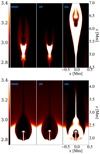 |
Fig. 14. AIA 193 Å images compared for all six models. Top row: for zrec = 2 Mm at time t = 622.6 s. Bottom row: zrec = 4.5 at time t = 389.1 s. The three panels are for MHD (left), 2fl (middle), and 2flα (right). Units are nondimensional. |
5. Summary
We ran simulations of two-fluid reconnection in a gravitationally stratified atmosphere, similar to the solar atmosphere, in which we studied the collisional effects for reconnection points situated at different heights. Because of the localized resitivity used, a Petschek-type reconnection developed, with slow shocks propagating along the x direction, disrupting the CS in a V shape. The vertical upward velocities of ≈10 km s−1 in the zrec = 2 Mm case and the width of the jets, which vary from being similar to the width of the CS (≈30 km) near the X point to ≈700 km higher up, due to the slow shocks, are consistent with properties of type-I spicules. The MHD and 2fl simulations show very similar results. When zrec = 4.5 Mm, the reconnection outflow hit the denser material below and interacted with the reconnected magnetic field, creating thin secondary CSs, leading to more locally turbulent behavior in the post-flare loop region.
The thermal effect of the collisions on the evolution of the neutral fluid had been observed earlier in simplified 1D slow-shock simulations, in which the heating of the neutrals produces an overshoot in the neutral velocity (Hillier et al. 2016; Snow & Hillier 2019). In our case, the decoupling is larger when the collisional effects are increased (in the 2flα cases) and the heating of the neutrals produces a runaway effect that separates the neutrals and the charges across the CS. The neutrals accumulate outside the CS, while the charges tend toward the center of the CS. This gives reversed contrasts in the charged density and neutral or total density maps. The regions with a very low density of neutrals have a high density of charges (inside the CS), and the regions with a very high density of charges have a low density of neutrals (outside the CS), and these differences increase over time. The temperature maps are consistent with the density maps, with high-density regions having low temperatures and low-density regions having high temperatures. This was analyzed in detail, and a nonlinear runaway decoupling effect was identified.
We obtain high reconnection rates in all the simulations because of the localized resistivity. The localized resistivity has the effect of bounding the current density, similar to an anomalous prescription. We obtain the maximum reconnection rate in the Petschek model, which is 0.1 (Vasyliunas 1975). Two-fluid effects do not increase our reconnection rates further, in contrast to the results of Leake et al. (2012, 2013). Our setup is closer to the conditions relevant for the stratified solar atmosphere.
Later on, we observed the formation of secondary plasmoids. They were observed in all models when zrec = 2 Mm. The large outflows and associated gradients in the flow when zrec = 4.5 Mm are likely inhibiting the linear tearing mode. This effect is much more important than collisions in the early formation of plasmoids. In simplified assumptions of uniform density, collisions define an effective density in the two-fluid model, similar to the idea presented by Murtas et al. (2021) in simulations of the coalescence instability. At later stages, however, the accumulation of plasma adds to the nonlinear evolution of the tearing mode. Because of a lower effective density when the collisional coupling is reduced, the effective Alfvén speed is higher and the simulations evolve slightly faster.
The secondary plasmoid formation process would look completely different in synthetic images that use total density instead of charged density in the calculation of emission in optically thin lines. When charged density is used in the synthetic-image generation, an MHD model that does not keep track of the ionization fraction produces slightly different results because of this limitation. It became evident that using charged-particle densities leads to more realistic behavior, in line with observed enhanced emission blobs.
Movies
Movie 1 associated with Fig. 3 (z2.0-2flalpha) Access Supplementary Material
Movie 2 associated with Fig. 3 (z2.0) Access Supplementary Material
Movie 3 associated with Fig. 9 (z4.5-2flalpha) Access Supplementary Material
Movie 4 associated with Fig. 9 (z4.5-bottom) Access Supplementary Material
When we use a purely Hydrogen plasma, the normalized mean molecular weights for charges and neutrals are uniform and constant (see Eq. (12) in Popescu Braileanu & Keppens 2022), being equal to 0.5 and 1, respectively.
Acknowledgments
This work was supported by the FWO grant 1232122N and a FWO grant G0B4521N. This project has received funding from the European Research Council (ERC) under the European Union’s Horizon 2020 research and innovation programme (grant agreement No. 833251 PROMINENT ERC-ADG 2018). This research is further supported by Internal funds KU Leuven, through the project C14/19/089 TRACESpace. The resources and services used in this work were provided by the VSC (Flemish Supercomputer Center), funded by the Research Foundation – Flanders (FWO) and the Flemish Government.
References
- Baty, H., Forbes, T. G., & Priest, E. R. 2014, Phys. Plasmas, 21, 112111 [NASA ADS] [CrossRef] [Google Scholar]
- Biskamp, D., & Schwarz, E. 2001, Phys. Plasmas, 8, 4729 [NASA ADS] [CrossRef] [Google Scholar]
- Bulanov, S. V., Syrovatskii, S. I., & Sakai, J. 1978, ZhETF Pisma Redaktsiiu, 28, 193 [NASA ADS] [Google Scholar]
- Close, R. M., Parnell, C. E., Longcope, D. W., & Priest, E. R. 2004, ApJ, 612, L81 [NASA ADS] [CrossRef] [Google Scholar]
- Del Zanna, G., Dere, K. P., Young, P. R., Landi, E., & Mason, H. E. 2015, A&A, 582, A56 [NASA ADS] [CrossRef] [EDP Sciences] [Google Scholar]
- Dover, F. M., Sharma, R., & Erdélyi, R. 2021, ApJ, 913, 19 [NASA ADS] [CrossRef] [Google Scholar]
- Furth, H. P., Killeen, J., & Rosenbluth, M. N. 1963, Phys. Fluids, 6, 459 [Google Scholar]
- Hillier, A., Takasao, S., & Nakamura, N. 2016, A&A, 591, A112 [NASA ADS] [CrossRef] [EDP Sciences] [Google Scholar]
- Innes, D. E., & Tóth, G. 1999, Sol. Phys., 185, 127 [NASA ADS] [CrossRef] [Google Scholar]
- Keppens, R., Popescu Braileanu, B., Zhou, Y., et al. 2023, A&A, 673, A66 [NASA ADS] [CrossRef] [EDP Sciences] [Google Scholar]
- Kumar, P., Karpen, J. T., Antiochos, S. K., et al. 2023, ApJ, 943, 156 [NASA ADS] [CrossRef] [Google Scholar]
- Leake, J. E., Lukin, V. S., Linton, M. G., & Meier, E. T. 2012, ApJ, 760, 109 [Google Scholar]
- Leake, J. E., Lukin, V. S., & Linton, M. G. 2013, Phys. Plasmas, 20, 061202 [NASA ADS] [CrossRef] [Google Scholar]
- Loureiro, N. F., Schekochihin, A. A., & Cowley, S. C. 2007, Phys. Plasmas, 14, 100703 [NASA ADS] [CrossRef] [Google Scholar]
- Manheimer, W. M., & Flynn, R. 1971, Phys. Rev. Lett., 27, 1175 [NASA ADS] [CrossRef] [Google Scholar]
- Martínez-Sykora, J., De Pontieu, B., Carlsson, M., et al. 2017, ApJ, 847, 36 [Google Scholar]
- Murtas, G., Hillier, A., & Snow, B. 2021, Phys. Plasmas, 28, 032901 [NASA ADS] [CrossRef] [Google Scholar]
- O’Flannagain, A., Brown, J., & Gallagher, P. 2015, ApJ, 799, 127 [CrossRef] [Google Scholar]
- Parker, E. N. 1957, J. Geophys. Res., 62, 509 [Google Scholar]
- Petschek, H. E. 1963, in The Physics of Solar Flares, Proceedings of the AAS-NASA Symposium held 28-30 October, eds. W. N. Hess (Washington, DC: National Aeronautics and Space Administration, Science and Technical Information Division), 425 [Google Scholar]
- Popescu Braileanu, B., & Keppens, R. 2022, A&A, 664, A55 [NASA ADS] [CrossRef] [EDP Sciences] [Google Scholar]
- Popescu Braileanu, B., Lukin, V. S., & Khomenko, E. 2023, A&A, 670, A31 [NASA ADS] [CrossRef] [EDP Sciences] [Google Scholar]
- Ruan, W., Xia, C., & Keppens, R. 2020, ApJ, 896, 97 [NASA ADS] [CrossRef] [Google Scholar]
- Ruan, W., Yan, L., & Keppens, R. 2023, ApJ, 947, 67 [NASA ADS] [CrossRef] [Google Scholar]
- Sato, T., & Hayashi, T. 1979, Phys. Fluids, 22, 1189 [NASA ADS] [CrossRef] [Google Scholar]
- Schmieder, B., Shibata, K., van Driel-Gesztelyi, L., & Freeland, S. 1995, Sol. Phys., 156, 245 [NASA ADS] [CrossRef] [Google Scholar]
- Schmieder, B., Joshi, R., & Chandra, R. 2022, Adv. Space Res., 70, 1580 [NASA ADS] [CrossRef] [Google Scholar]
- Snow, B., & Hillier, A. 2019, A&A, 626, A46 [NASA ADS] [CrossRef] [EDP Sciences] [Google Scholar]
- Snow, B., & Hillier, A. 2021, A&A, 645, A81 [EDP Sciences] [Google Scholar]
- Song, P., Tu, J., & Wexler, D. B. 2023, ApJ, 948, L4 [NASA ADS] [CrossRef] [Google Scholar]
- Sweet, P. A. 1958, in Electromagnetic Phenomena in Cosmical Physics, ed. B. Lehnert, 6, 123 [NASA ADS] [Google Scholar]
- Takasao, S., Isobe, H., & Shibata, K. 2013, PASJ, 65, 62 [Google Scholar]
- Takasao, S., Matsumoto, T., Nakamura, N., & Shibata, K. 2015, ApJ, 805, 135 [NASA ADS] [CrossRef] [Google Scholar]
- Ugai, M. 1995, Phys. Plasmas, 2, 388 [NASA ADS] [CrossRef] [Google Scholar]
- Uzdensky, D. A. 2003, ApJ, 587, 450 [NASA ADS] [CrossRef] [Google Scholar]
- Vasyliunas, V. M. 1975, Rev. Geophys. Space Phys., 13, 303 [CrossRef] [Google Scholar]
- Vernazza, J. E., Avrett, E. H., & Loeser, R. 1981, ApJS, 45, 635 [Google Scholar]
- Wang, Y., Cheng, X., Ding, M., & Lu, Q. 2021, ApJ, 923, 227 [NASA ADS] [CrossRef] [Google Scholar]
- Xia, C., Teunissen, J., El Mellah, I., Chané, E., & Keppens, R. 2018, ApJS, 234, 30 [Google Scholar]
- Yadav, N., Keppens, R., & Popescu Braileanu, B. 2022, A&A, 660, A21 [NASA ADS] [CrossRef] [EDP Sciences] [Google Scholar]
- Yamada, M., Kulsrud, R., & Ji, H. 2010, Rev. Modern Phys., 82, 603 [NASA ADS] [CrossRef] [Google Scholar]
- Yokoyama, T., & Shibata, K. 1996, PASJ, 48, 353 [Google Scholar]
- Zanna, L. D., Landi, S., Papini, E., Pucci, F., & Velli, M. 2016, J. Phys. Conf. Ser., 719, 012016 [NASA ADS] [CrossRef] [Google Scholar]
Appendix A: Linear tearing in two-fluid settings
The linearized, incompressible, resistive MHD equations, in which the background density, ρ0, is uniform, the background magnetic field, B0 = (0,By0(x),Bz0(x)), is force-free, and the evolution of the perturbed magnetic field, B1, neglects the changes resulting from the Ohmic diffusion of the equilibrium magnetic field, are
 (A.1)
(A.1)
 (A.2)
(A.2)
and
 (A.3)
(A.3)
In these equations, J1 = ∇ × B1 is the perturbed current. In a 2.5D geometry (xz plane), we considered the y component after taking ∇× of Eq. A.1, the x component of Eq. A.2, and
 (A.4)
(A.4)
which is equivalent in the linear assumption to the z component of Eq. A.2. After assuming a solution of the form {vx(x, z, t),Bx1(x, z, t)} = {ux(x),bx(x)} ⋅ exp(γt − ikzz), the following system was obtained (see also Furth et al. 1963; Zanna et al. 2016; Loureiro et al. 2007):
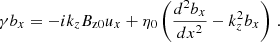
![Mathematical equation: $$ \begin{aligned}&i \gamma \rho _0 \left(\frac{d^2 u_x}{d x^2} - k_z^2 u_x\right) = \nonumber \\&\quad \quad \quad k_z \left[ B_{\rm z0} \frac{d^2 b_x}{d x^2} - b_x \left( k_z^2 B_{\rm z0} + \frac{d^2 B_{\rm z0}}{d x^2}\right) \right]\,, \end{aligned} $$](/articles/aa/full_html/2023/10/aa46659-23/aa46659-23-eq23.gif) (A.5)
(A.5)
 (A.6)
(A.6)
In the two-fluid model, when there are separate momentum equations for charges and neutrals, Eqs. A.1- A.3 are replaced by:
 (A.7)
(A.7)
 (A.8)
(A.8)
 (A.9)
(A.9)
and
 (A.10)
In the two-fluid assumption, Eq. A.6 remains unmodified, and Eq. A.5 can be rewritten, so we thus get the following coupled system of two governing, linear, ordinary differential equations:
![Mathematical equation: $$ \begin{aligned}&i \gamma \rho (\gamma ) \left(\frac{d^2 u_x}{d x^2} - k_z^2 u_{\rm cx}\right) = \nonumber \\&\quad \quad \quad k_z \left[ B_{\rm z0} \frac{d^2 b_x}{d x^2} - b_x \left( k_z^2 B_{\rm z0} + \frac{d^2 B_{\rm z0}}{d x^2}\right) \right]\,,\end{aligned} $$](/articles/aa/full_html/2023/10/aa46659-23/aa46659-23-eq29.gif) (A.11)
(A.11)
 (A.12)
in which
 (A.13)
and ρT0 = ρc0 + ρn0 is the background total density. Since for every γ we have ρc0 ≤ ρ(γ)≤ρT0, this defines an effective density in the two-fluid model, based on the collisional coupling α.
We observed in Fig. 11 that all plasmoids that formed have a similar length scale, estimated as λ ≈ 0.3 Mm. We considered the densities at z = 3.5 Mm, the value of the resistivity η0 = 8 Ωm, and solved numerically (using the Python NumPy solver) the eigenvalue problem resulting from the spatial discretization of Eqs.(A.5) and (A.6), with boundary conditions whereby we set both variables to zero, and thus obtaining the growth rate in the MHD assumption. In doing so, we found that the largest growing mode (with a wavelength larger than 0.1 Mm and smaller than 0.5 Mm) has wavelength λ = 0.4 Mm for the parameters considered. The density-gradient scale height is, at z = 3.5 Mm, much larger than the vertical size of the domain and than the wavelength considered, which justifies neglecting the gravity and all variations in the quantities in the vertical direction.
Fig. A.1 shows the computed growth rate as a function of density (varying between ρc0 ≤ ρ ≤ ρT0) for the MHD case, and also gives the two-fluid growth rate for several values of α as indicated in the legend. To get the solid black line in Fig. A.1 which quantifies growth rates in the MHD approximation, we fixed λ = 0.4 Mm and numerically solved the eigenvalue problem in the MHD approximation for densities with values between the charged density and the total density. The growth in the two-fluid approach is at the intersection points between the black line and the curve of ρ−1, the inverse of ρ(γ) from Eq.(A.13), (only the intersection points are shown in Fig. A.1 and not the curve ρ−1).
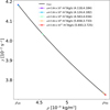 |
Fig. A.1. Growth rate and effective density for the tearing mode with wavelength = 0.4 Mm, the fastest growing mode for η0 = 8 Ωm, and densities at z = 3.5 Mm. The growth rate obtained in the MHD approximation is shown by a solid black line. The growth rates in the two-fluid approach are located on this line, depending on the value of the collisional parameter α. Several values of α are considered, as indicated in the legend in which we also show the (ρ, γ) coordinates of the points in brackets. |
All Figures
|
Fig. 1. Initial profiles as a function of height. For the densities, neutrals (dashed blue line), charges (dotted red line), and the total (solid black line) are on the left axis. The temperature (solid orange line) is on the right axis. |
| In the text | |
|
Fig. 2. Collisional mean-free paths as functions of height. We show the mean-free paths between ions and neutrals (λin, red lines) and between neutrals and ions (λni, blue lines) for the two collisionality regimes considered: self-consistent from plasma-neutral parameters (2fl, solid lines, left axis) and reduced-case 2flα (dashed and dotted lines, right axis, with a different order of magnitude). The collisional mean-free paths were calculated according to Eq. (8). |
| In the text | |
|
Fig. 3. Time evolution of the total density for all six simulations. Left panels: zrec = 2 Mm. Right panels: zrec = 4.5 Mm. A different physics model is shown in each row: MHD (top row), 2fl (middle row), and 2flα (bottom row). An online animation (case z2.0-2flalpha.mp4 or 2flα) overplots the adaptive grid for the neutral density. |
| In the text | |
|
Fig. 4. Comparison between the out-of-plane current density. For two-fluid models: 2fl (left) and 2flα (right) at t = 622.6 s. Black lines with arrows are magnetic field lines. Yellow-to-green colored contours relate to the density variation. The ripple in the magnetic field, associated with the reversal in the Bz sign, located at z ≈ 5 Mm, is indicated in the figure. |
| In the text | |
|
Fig. 5. Comparison between the charged densities (top panels) and the neutral densities (bottom panels) for t = 622.6 s. Top row: 2fl (left panel), 2flα (middle panel), and MHD with charged fluid only (right panel). Bottom row: 2fl (left panel) and 2flα (right panel). |
| In the text | |
|
Fig. 6. Comparison between the temperatures of neutrals and charges at t = 622.6 s. Top panels: 2f. Bottom panels: 2flα. |
| In the text | |
|
Fig. 7. Horizontal cut at coronal height z = 4 Mm at time t = 622.6 s for the simulations with TR reconnection or zrec = 2 Mm. (a) Density of charges. (b) Density of neutrals. (c) x velocity for charges and neutrals. (d) Temperature of charges and neutrals. (e) Total density. (f) Center of mass temperature from Eq. (10). Different curves are for the two models considered – 2fl and 2flα – quantities for charges and neutrals are shown in the same plot in panels c and d, as indicated in the legend. The primary and secondary maximum peaks in the neutral collisional heating term for case 2flα, as shown in detail in Fig. 8 and located at z = −0.03 Mm and z = −0.1 Mm, are indicated by vertical violet and dotted gray lines, respectively. |
| In the text | |
|
Fig. 8. Horizontal cuts along z = 4 Mm for the case with TR reconnection, or zrec = 2 Mm at time t = 622.6 s, the same time as for Fig. 7. Quantities corresponding to charged and neutral fluid are shown with red lines and blue lines, respectively. Left panels: 2fl case. Right panels: 2flα case. Top row: Terms in the temperature equation; the Ohmic term (solid red line) and collisional heating terms (dashed lines: red for charges and blue for neutrals). Bottom row: Terms in the velocity equation; acceleration is due to magnetic pressure (dashed red line), the gas-pressure gradient (solid lines; red for charges and blue for neutrals), and collisions (dotted lines; red for charges and blue for neutrals). The primary and secondary maximum peaks in the collisional heating associated with neutrals, located (and shown only for negative x, because of symmetry) at z = −0.03 Mm and z = −0.1 Mm, are indicated by vertical dotted violet and gray lines, respectively, for the 2flα case (right panels). |
| In the text | |
|
Fig. 9. Two-fluid coronal-reconnection downflows impacting the chromosphere. We provide snapshots of charged density (top left), neutral density (top right), out-of-plane current density (bottom left), and charged temperature (bottom right) for the simulation zrec = 4.5 Mm, with 2flα at t = 591.5 s; the last time shown is in the right column at the bottom of Fig. 3. In the panels of neutral and charged densities (top panels), the orange arrows show the velocities of neutral and charged fluid, respectively. We overplot the magnetic field lines and the decoupling velocities over the current density map (bottom-left panel) and isocontours of the temperature decoupling (Tc − Tn) in the range −1.8 × 10⁶ K and 1.8 × 10⁶ K over the charged temperature image (bottom-right panel). |
| In the text | |
|
Fig. 10. Reconnection rates for the six simulations as a function of time. The two cases of reconnection height are considered: zrec = 2 Mm (left panel) and zrec = 4.5 Mm (right panel). Different curves indicate different models: MHD (solid orange line), 2fl (dashed green line), and 2flα (dotted blue line). |
| In the text | |
|
Fig. 11. Vertical profiles of the vertical velocity when the plasmoids form for zrec = 2 Mm. Shown for five moments in time in the late stage of the simulations, for the three models: 2flα (left panel), 2fl (middle panel), and MHD (right panel). For the two-fluid models (left and middle panels), we show the velocity of charges. The linear fit of the velocity profile around the reconnection point (where the velocity changes sign) is shown by a black line and the value of the slope is indicated at the top of each panel. |
| In the text | |
|
Fig. 12. AIA 193 Å response function R(T) as a function of temperature (measured in K), (Del Zanna et al. 2015). Both axes are logarithmic. |
| In the text | |
|
Fig. 13. Synthetic views on secondary plasmoids, at three consecutive times. For plasmoids in the case zrec = 2 Mm, we show synthetic images of AIA 193 Å emission. Top row: 2fl case. Middle and bottom rows: 2flα case. For the calculation of emission, we used the density and temperature of charges in the top and middle row, and the total density and the center of mass temperature of neutrals and charges in the bottom row. The units are nondimensional. We kept the colorbar in the figures, for comparison purposes, as normalization is done in the same way. The last row shows different limits on the colorbar because of the increased density when the total density is considered instead of the charged particles only. |
| In the text | |
|
Fig. 14. AIA 193 Å images compared for all six models. Top row: for zrec = 2 Mm at time t = 622.6 s. Bottom row: zrec = 4.5 at time t = 389.1 s. The three panels are for MHD (left), 2fl (middle), and 2flα (right). Units are nondimensional. |
| In the text | |
|
Fig. A.1. Growth rate and effective density for the tearing mode with wavelength = 0.4 Mm, the fastest growing mode for η0 = 8 Ωm, and densities at z = 3.5 Mm. The growth rate obtained in the MHD approximation is shown by a solid black line. The growth rates in the two-fluid approach are located on this line, depending on the value of the collisional parameter α. Several values of α are considered, as indicated in the legend in which we also show the (ρ, γ) coordinates of the points in brackets. |
| In the text | |
Current usage metrics show cumulative count of Article Views (full-text article views including HTML views, PDF and ePub downloads, according to the available data) and Abstracts Views on Vision4Press platform.
Data correspond to usage on the plateform after 2015. The current usage metrics is available 48-96 hours after online publication and is updated daily on week days.
Initial download of the metrics may take a while.