| Issue |
A&A
Volume 676, August 2023
|
|
|---|---|---|
| Article Number | A117 | |
| Number of page(s) | 11 | |
| Section | Numerical methods and codes | |
| DOI | https://doi.org/10.1051/0004-6361/202346086 | |
| Published online | 22 August 2023 | |
Simplifying asteroseismic analysis of solar-like oscillators
An application of principal component analysis for dimensionality reduction
1
School of Physics and Astronomy, University of Birmingham,
Birmingham
B15 2TT, UK
e-mail: This email address is being protected from spambots. You need JavaScript enabled to view it.
2
Advanced Research Computing, University of Birmingham,
Birmingham
B15 2TT, UK
3
Institute for Astronomy, University of Hawai‘i,
2680 Woodlawn Drive,
Honolulu, HI
96822, USA
Received:
6
February
2023
Accepted:
11
June
2023
Abstract
Context. The asteroseismic analysis of stellar power density spectra is often computationally expensive. The models used in the analysis may require several dozen parameters to accurately describe features in the spectra caused by the oscillation modes and surface granulation. Many of these parameters are often highly correlated, making the parameter space difficult to quickly and accurately sample. They are, however, all dependent on a much smaller set of parameters, namely the fundamental stellar properties.
Aims. We aim to leverage this to develop a method for simplifying the process of sampling the model parameter space for the asteroseismic analysis of solar-like oscillators, with an emphasis on mode identification.
Methods. Using a large set of previous observations, we applied principal component analysis to the sample covariance matrix to select a new basis on which to sample the model parameters. Selecting the subset of basis vectors that explains the majority of the sample variance, we then redefined the model parameter prior probability density distributions in terms of a smaller set of latent parameters.
Results. We are able to reduce the dimensionality of the sampled parameter space by a factor of two to three. The number of latent parameters needed to accurately model the stellar oscillation spectra cannot be determined exactly but is likely only between four and six. Using two latent parameters, the method is able to produce models that describe the bulk features of the oscillation spectrum, while including more latent parameters allows for a frequency precision better than ≈10% of the small frequency separation for a given target.
Conclusions. We find that sampling a lower-rank latent parameter space still allows for accurate mode identification and parameter estimation on solar-like oscillators over a wide range of evolutionary stages. This allows for the potential to increase the complexity of spectrum models without a corresponding increase in computational expense.
Key words: asteroseismology / stars: oscillations / methods: data analysis / methods: statistical
Hubble Fellow.
© The Authors 2023
 Open Access article, published by EDP Sciences, under the terms of the Creative Commons Attribution License (https://creativecommons.org/licenses/by/4.0), which permits unrestricted use, distribution, and reproduction in any medium, provided the original work is properly cited.
This article is published in open access under the Subscribe to Open model. This email address is being protected from spambots. You need JavaScript enabled to view it. to support open access publication.
1 Introduction
Asteroseismology is the process of measuring the oscillation frequencies of stars. This is typically done by first observing the flux or radial velocity variations due to the oscillations on the stellar surface, and then analyzing the power spectral density (PSD) of the time series. The properties of the spectrum, including the oscillation frequencies, allow for quantities such as the stellar mass, radius, and age to be precisely measured (see, e.g., Silva Aguirre et al. 2017; Cunha et al. 2021). Solar-like oscillators in particular are numerous and ubiquitous along the lower main sequence and during the red-giant evolutionary phases (Chaplin et al. 2014; Yu et al. 2018; Hon et al. 2019; Hatt et al. 2023). The oscillations therefore yield constraints on a wide range of physics in the stars themselves, but also in any orbiting companions and the environments they are embedded in, such as stellar clusters and associations.
Solar-like oscillators pulsate due to standing waves that permeate the stellar interior (see, e.g., Chaplin & Miglio 2013). The restoring force for these oscillations is the gradient of pressure, and so these standing waves are often simply called p modes. Many modes can be excited simultaneously and thus become visible on the stellar surface, and each one is distinguished by its spherical harmonic angular degree, l, and azimuthal order, m, as well as a radial order, n. The most readily visible asteroseismic quantities are the regular spacing, Δν, of the mode peaks and the frequency of maximum power, νmax. Measuring these global asteroseismic properties is computationally inexpensive (see, e.g., Chontos et al. 2021; Hatt et al. 2023) but is sufficient for determining the stellar mass and radius to a precision of a few percent (Chaplin et al. 2014). These features of the oscillation spectrum have been shown to strongly depend on the bulk stellar properties, such as the surface gravity and effective temperature (Kjeldsen & Bedding 1995), with additional variance potentially due to metallicity (Viani et al. 2017; Li et al. 2022).
The precision on the inferred stellar properties is increased by measuring the individual mode frequencies (see, e.g., Lebreton & Goupil 2014). This involves first identifying which oscillations are present in the PSD by assigning an angular degree and radial order of the mode. This can then be followed by evaluating the likelihood of a detailed spectrum model that includes information about the mode amplitudes and lifetimes in addition to the precise mode frequencies. For long, high-cadence time series such as those from the CoRoT (Baglin et al. 2009), Kepler (Borucki et al. 2010) and Transit Exoplanet Survey Satellite (TESS; Ricker et al. 2015) missions, this process may become computationally expensive. Part of this computational expense comes from the quantity of the data, but a non-negligible expense also comes from the overall shape and volume of the posterior probability density function. Depending on the required precision and quantities of interest, the spectrum models may include anywhere from ~10–100 parameters (see, e.g., Appourchaux et al. 2012; Davies et al. 2016; Lund et al. 2017; Benomar et al. 2018; Hall et al. 2021). These parameters all depend on the same fundamental stellar properties, and many of them are highly correlated. High-dimensional, highly correlated posterior distributions are often difficult to map, thereby adding to the computational expense of measuring the oscillation parameters.
Problems involving parameterized models with many correlated parameters are amenable to dimensionality reduction (DR) methods. These methods seek to identify a lower-rank, latent parameter space that may be more directly related to an underlying set of physical parameters. For asteroseismology, the application of DR methods can simplify the process of mode identification by mapping the smaller, latent parameter space, rather than a model parameter space that consists of dozens of parameters. Several methods exist for performing DR, such as feature selection (Guyon & Elisseeff 2003), autoencoders (Goodfellow et al. 2016; Kingma & Welling 2013), and matrix factorization (Lee & Seung 1999). Here we demonstrate the use of principal component analysis (PCA) for DR to simplify the process of performing mode identification and extracting information from the oscillation spectrum of solar-like oscillators. Briefly, given a sample of observational measurements of the spectrum model parameters, the PCA method decomposes the sample covariance matrix into a set of eigenvectors with associated eigenvalues. Each eigenvector explains a fraction of the total variance in the sample, and those that explain the majority of the variance are assumed to predominantly represent real correlations between parameters. The remaining eigenvectors, which explain the least amount of variance, are likely due to noise in the measurements and are discarded. This yields a reduced parameter space from which samples can be drawn, which can be projected back into the full parameter space to subsequently evaluate the model likelihood given an observed PSD spectrum. We leverage this to simplify the process of mode identification by using a generative spectrum model, where the parameters are known to correlate with the stellar fundamental parameters.
In Sect. 2, we briefly summarize the spectrum model, which is based on the PBjam model used by Nielsen et al. (2021) but extended to include additional background noise terms. In Sect. 3, we describe how we use PCA to perform DR and its application to mode identification in asteroseismology. The performance of the method is shown in Sect. 4, followed by concluding remarks in Sect. 5.
2 The full spectrum model
Modeling the stellar oscillation spectrum is typically performed by drawing samples from the posterior distribution,
 (1)
(1)
where ℒ(S|Θ) is the likelihood of observing the PSD spectrum, S, given a spectrum model that is a function of the set of parameters Θ, and 𝒫(Θ) is the prior representing our current knowledge of these parameters. By sampling the parameters of a generative spectrum model where the modes appear with a known pattern, we can evaluate the probability that an observed peak in the spectrum is due to a mode from the model and thereby assign a label of n and l.
The parameter space is typically sampled using an Markov chain Monte Carlo approach (e.g., Handberg & Campante 2011; Lund et al. 2017) or nested sampling methods (Corsaro et al. 2020). In the following we use nested sampling, as this has been shown to perform well with multi-modal posterior distributions, which, depending on the chosen model, may be the case in a PSD spectrum with multiple resolved modes (Buchner et al. 2014). We used the Dynesty (Speagle 2020) package to perform nested sampling (Skilling 2004). This is, however, not a strict requirement and the presented method for DR is applicable to other types of sampling or optimization methods.
Here we restricted ourselves to using a PSD model equivalent to that used by Nielsen et al. (2021), with additional terms to describe the background power density not directly attributable to the oscillations. The spectrum model is defined as
 (2)
(2)
 (3)
(3)
Here the first sum is over the visible number of radial orders NO and consists of Lorentzian profiles describing the power density of each oscillation mode. The modes are characterized by their radial order n and angular degree l, and the sum consists of pairs of modes defined by (n, l = 0) and (n − 1, l = 2). The frequencies are parameterized by the asymptotic relation (see, e.g., Mosser et al. 2015)
 (4)
(4)
where ε is a phase term, nmax = νmax/∆ν − ε, and α is the scale of the second order mode frequency variation. The frequencies of the l = 2 modes are offset from the l = 0 modes by the small frequency separation δν02, which is kept as a free parameter but is identical for all mode pairs. The mode heights are parameterized by a Gaussian,
 (5)
(5)
with a height HE, a width WE, and is centered on νmax. The heights, hn−1,2, of the quadrupole modes are approximated as a fraction of the l = 0 mode height, determined by the relative mode visibility. Here this fraction was set to 0.7, which is appropriate for Kepler observations (Handberg & Campante 2011). Finally, we used a single value of the mode width Γ for all the observed modes.
The l = 1 modes were omitted from the spectrum model since it is difficult to establish a precise and comprehensive description of their mode frequencies for a wide range of evolutionary stages. In addition we also did not consider modes of l = 3 since these are typically only visible in the brightest targets. Inclusion of l = 1 and l = 3 modes is left for future work.
The last two parts of Eq. (2) consist of the frequency-independent white noise level, W, and a number, NB, of frequency-dependent background noise terms. The background terms are described by Lorentzian-like profiles centered on ν = 0 (Harvey 1985; Kallinger et al. 2014). Each term has an amplitude, ai, a frequency, bi, and an exponent, ci, which governs the decrease in the noise power with frequency. We used three background terms: The first two are typically attributed to the appearance of granulation on the stellar surface, and are most apparent in the spectrum at a characteristic frequency comparable to νmax and at ≈0.3νmax, respectively. The third and lowest frequency term captures the combination of variability caused by, for example, long-term instrumental effects and stellar activity, which tend to dominate the PSD at frequencies ≲1 μHz. An example of the spectrum model for the red giant ϵ Reticuli is presented in Fig. 1, where we show the individual components of the background model along with the combined spectrum model.
The inclusion of the background term was motivated by the necessity to accurately model the background noise that the oscillation modes are embedded in. In addition, just like the oscillation modes, the granulation on the stellar surface that causes the background noise stems from convective processes in the star. The background noise parameters are therefore correlated with those of the oscillation modes, and so indirectly constrain the mode parameters (see, e.g., Kjeldsen & Bedding 2011; Chaplin et al. 2011).
The power density is χ2-distributed with two degrees of freedom. Given the model, M, in Eq. (2) we can then write the log-likelihood function as (see, e.g., Woodard 1984; Duvall & Harvey 1986)
 (6)
(6)
where S is the observed power density spectrum, and J is the total number of frequency bins in the spectrum. As in Nielsen et al. (2021), we added an additional likelihood term, In ℒobs(d|θ), which is the likelihood due to additional observational constraints, d, that are not directly part of the spectrum model. In this case ℒobs(d|θ) is the joint probability given by normal distributions centered on the observed Teff and de-reddened GBP − GRP, with a standard deviation corresponding to the respective uncertainties. We use values from Evans et al. (2018) in the following analysis.
For clarity in the following we have separated the set of parameters Θ = {Δν, νmax, ε, δν02, α, HE, WE, Teff, GBP − GRP, Γ, ai, bi, ci, W} into two subsets θ and ϕ. The subset θ are those parameters in Θ that we expect are predominantly functions of the intrinsic stellar parameters, whereas those in ϕ are functions that are dominated by extrinsic variability such as instrumental noise. We only applied DR to θ as these are the parameters that are expected to be most strongly correlated with the stellar properties. These parameters are: all the mode parameters, those of the two high frequency Harvey-like background noise terms, and Teff and GBP − GRP. The parameters ϕ (see Table 1) are the photon shot noise and the lowest-frequency background noise term. While these are to some extent correlated with the physical stellar properties, they are also strongly affected by instrumental effects such as the choice of pixel mask, pixel sensitivity, and observation duration. We therefore left these parameters out of the DR. This means that we have 16 parameters that are amenable to DR and four that are left as independent random variables in the sampling.
 |
Fig. 1 Example spectrum of the red giant ϵ Reticuli. The PSD is shown in light and dark gray (smoothed). The components of the background model are shown with dashed lines, while the combined spectrum model, including the mode components, is shown in red. The parameters of the spectrum model are drawn from the prior sample around νmax ≈ 300 μHz the equivalent to that of ϵ Reticuli. |
Additional model parameter priors.
3 Defining the model parameter priors
Given the log-likelihood in Eq. (6) we next needed to define the prior probability density 𝒫(Θ). We present the functions used as priors for ϕ in Table 1. For a3 in the instrumental background term and the white noise level, W, we used a normal distribution in logarithmic power. These distributions are centered on the means μp and μW, respectively, which are determined by the power in the first and last few frequency bins of the spectrum. For the characteristic frequency b3, the prior is a normal distribution in log b3, centered on 1 μHz with a width of 0.15 dex. We used a β distribution with shape parameters α = 1.2 and β = 1.2 for the exponent in the background term, where we set the location and scale parameters to one and three, respectively.
Next we needed to determine the prior probability densities for the parameter θ that are included in the DR. We started by using a large sample of measurements of θ, which is based on that of Nielsen et al. (2021) and consists of the 16 model parameters for 13 443 targets observed in 30-min and 58-s cadences by Kepler and 2-min cadence by TESS. Our assumption here is that, using PCA on the sample covariance matrix, it is possible to identify a set of latent variables,  , which is likely of smaller dimension than θ. The prior density is then defined in terms of
  instead of θ by projecting the original prior sample into the latent parameter space, and then approximating that distribution by a kernel density estimate (KDE).
3.1 Computing the weighted covariance matrix
Given an N × D matrix, θ, consisting of N observations of the D = 16 model parameters, we first computed the weighted covariance matrix,
 (7)
(7)
where θ′ is θ translated and scaled to zero mean and unit standard deviation in each column. The matrix W is an N × N diagonal matrix with elements wn, which are the weights on each individual observation of the model parameters. We did not consider the more general case of different sets of weights for each parameter and observation as this does not allow for a simple analytical method of determining the principal components (see, e.g., Tamuz et al. 2005).
Since PCA minimizes the variance of a given sample along each of the principal components, the proposed method has two shortcomings that the row weights wn can be used to mitigate. First, PCA is sensitive to outliers in the sample. This can be treated by assigning low weights relative to the remainder of the sample. We do not identify outliers here as the sample of observations has been previously vetted manually. Secondly, PCA is less effective as a DR method if parameters in the sample are nonlinearly correlated, which is the case for our sample of model parameters since it spans a wide range of evolutionary stages. For example, the dependence of ε in Eq. (4) on Teff changes significantly between main-sequence and red-giant stars (see, e.g., White et al. 2012).
However, these nonlinear effects in the parameter correlation are reduced when only considering targets that are similar to the target of interest. This is done by setting the row weights wn such that they are unity for targets in a small volume around the expected target parameters, and zero elsewhere. This small volume of targets is defined by using the K nearest neighbors in terms of the Euclidean distance between the estimated target values of νmax, Teff, and GBP − GRP, and those of the prior sample. Figure 2 illustrates the process of selecting subsamples around a notional target with νmax ≈ 830 μHz, Teff ≈ 5640 K, and GBP − GRP ≈ 0.86. In this case, the correlation is strongly nonlinear on the ϵ and log νmax plane over large ranges of νmax, but for decreasing K the correlation becomes predominantly linear.
We find that with the current sample of prior observations, the method is insensitive to the exact choice of K, which can be ~10–1000. This selection scheme does require some prior knowledge of νmax for the target. However, this can be estimated to within a few percent by for example fitting simple models to the PSD (e.g., Huber et al. 2011; Chontos et al. 2021), or to within ~10% by using the asteroseismic scaling relations (Kjeldsen & Bedding 1995) along with an approximate stellar radius from parallax and broad-band photometry (see, e.g., Campante et al. 2019; Hatt et al. 2023).
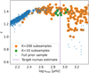 |
Fig. 2 ϵ and log νmax values for a selection of the K = 10 (green) and K = 200 (orange) nearest neighbors, determined by the Euclidean distance relative to an example target with a notional νmax ≈ 830 μHz (horizontal purple line), an effective temperature Teff ≈ 5640 K, and GBP − GRP ≈ 0.86. |
3.2 Sampling the latent parameter space
The principal components are found by identifying the eigenvectors, Q, by factoring C as
 (8)
(8)
where the columns of Q are the eigenvectors (principal components), and the diagonal matrix Λ consists of their eigenvalues. We used the Numpy library (Harris et al. 2020) to perform the eigendecomposition.
The set of eigenvectors, Q, forms a new basis for the sample, where each axis corresponds to a latent variable. Any given set of observations  can subsequently be projected onto the new basis by
 (9)
(9)
Conversely, a sample drawn from the eigenvector space can be projected back to the model parameter space by
 (10)
(10)
Using Eq. (9), we can transform draws from the prior sample in the model parameter space, into the latent parameter space to show their distribution on the new basis. Figure 3 shows 400 draws from around νmax = 100 μHz projected onto a subset of the new basis. We can use the distribution of these samples to approximate what the prior density looks like in the latent space, and subsequently start drawing new samples from this latent prior density.
For simplicity, we only considered the marginalized distributions of the projected prior, where we used a one-dimensional KDE to approximate the distribution of each latent parameter. As seen by the marginal distribution of θ2, for example, this approach can lead to a small loss of accuracy in representing details such as multi-modality, which is caused by selecting a large KDE bandwidth. However, as shown in the right set of frames in Fig. 3 the original prior sample is still well represented by this sample when projected into the model parameter space using Eq. (10). Sharp features such as discontinuities in the model parameter prior are however not well captured by this method, as indicated by the marginal distributions of νmax. This loss of fidelity around sharp features in the prior samples simply translates into a reduction in efficiency of the sampling, since more samples will be drawn from areas of parameter space that the prior sample suggests should be improbable.
The eigenvalues determine the amount of the total variance in the sample that is explained by each corresponding eigenvector. The eigenvectors that explain the majority of the correlation can therefore be chosen by selecting the d vectors with the highest eigenvalues, where the variance along the remaining eigenvectors is assumed to be due to noise. Figure 4 shows an example of the eigenvalues of C ordered according to value. In this case the majority of the variance is explained by the eigenvectors associated with the first few eigenvalues, while including additional eigenvectors accounts for comparatively less variance.
Picking a number, d, of eigenvectors where d < D, necessarily means discarding information from the sample corresponding to the missing variance along the remaining D − d vectors. The amount of variance retained by a choice of d is shown by the cumulative explained variance shown in Fig. 5, where the variation in νmax is due to the local density and covariance of the prior sample targets.
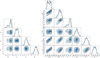 |
Fig. 3 Corner plots of a sample of 400 targets around νmax = 100 μHz drawn from the prior distribution. Left: projection of the sample into the latent parameter space (in black) and a corresponding sample (in blue) drawn from the one-dimensional KDE approximations of the marginalized distributions (diagonal frames). Right: original 400 prior sample draws (in black) with the sample drawn from the latent space, projected into the model parameter space (in blue). For clarity we only show a subset of the model parameters, where all parameters except ε are in base-10 logarithmic units. |
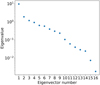 |
Fig. 4 Eigenvalues of a covariance matrix computed from 400 samples of θ around and input νmax = 100 μHz where θ consists of 16 parameters. The eigenvalues are ordered by descending value, and the first few corresponding eigenvectors explain the majority of the sample variance. |
 |
Fig. 5 Cumulative explained variance of 400 samples of θ for different combinations of input νmax and selected eigenvectors. The dashed line indicates the delineation between stars observed in Kepler long cadence (low frequency) and short cadence (high frequency). The effective covariance matrix rank is indicated in red, and the number of latent parameters suggested by Jolliffe’s modified KG criterion is shown in purple. |
3.3 Picking the number of latent parameters
From a data-driven perspective, it is possible to estimate the approximate value of d with several different methods (see, e.g., Cangelosi & Goriely 2007, for a comparison of several methods). Here, we show the use of two such methods: Jolliffe’s modification to the Kaiser-Guttman (KG; Guttman 1954; Kaiser 1960; Jolliffe 1972) criterion and the effective matrix rank estimation.
The KG criterion suggests using eigenvectors of the correlation matrix1 with eigenvalues greater than 1, since these explain variance in the model space corresponding to more than one parameter. Jolliffe (1972) later found that using eigenvalues greater than 0.7 is more appropriate based on simulated data sets, since this retains a greater fraction of the total variance and so potentially discarding less information.
An alternative to the KG criterion is the effective covariance matrix rank, E, which is related to the entropy of the eigenvalues (Roy & Vetterli 2007) and is given by
![Mathematical equation: $E = \exp \left[ { - \sum\limits_{d = 1}^D {{\lambda _d}\ln {\lambda _d}} } \right],$](/articles/aa/full_html/2023/08/aa46086-23/aa46086-23-eq14.png) (11)
(11)
where  , and the exponent is the Shannon entropy (Shannon 1948) of the eigenvalues. The effective rank is a non-integer value that approaches 1 when the entropy of the eigenvalues is large, which corresponds to only a few eigenvalues explaining most of the variance. Conversely, the effective rank approaches D when all the eigenvalues entropy is small, meaning they are all equally important.
In Fig. 5, we compare the number of eigenvectors suggested by both methods with the cumulative explained variance. While these two methods suggest different numbers for the eigenvectors to retain, the typical value for our sample is between four and eight, which corresponds to explaining 80–90% of the total sample variance, with the effective matrix rank method suggesting ten latent parameters is necessary between νmax ≈ 100 μHz and 200 μHz.
However, neither the effective covariance matrix rank nor the modified KG criterion use any physical information about the model parameters involved. It is typically assumed, in the statistical modeling of the structure and evolution of solar-like oscillators, that the observed parameters generated by a star can be described using only a handful of fundamental parameters. By accepting a certain level of uncertainty, it is possible, for example, to describe a star and thereby the predicted mode frequencies using just its initial mass, initial metallicity, and current age. This assumes a degree of simplification, for example a known helium enrichment law, or other initial chemical relation in r-process elements. If we were to relax these assumptions to achieve a higher degree of accuracy, we then introduce additional parameters to describe the observed properties of the star.
This process of relaxing assumptions and adding more parameters can in principle be continued to reach a greater degree of detail, at the cost of making the stellar model more complex. However, an analogous study with numerical models of stellar structure (which we describe in more detail in Appendix A) indicates that perhaps five or so free parameters are already more than sufficient to describe the effects on the mode frequencies of changing a larger number of parameters of these models, associated with quite different physical processes and properties. While the stellar model parameters are not the same as the latent parameters identified by the PCA method, the precision achieved by stellar modeling with just five parameters suggests that the number of sufficient latent parameters is substantially smaller than the 16 model parameters, and possibly very similar.
4 Performance of the PCA method
Our physical motivation suggests that the number of latent parameters should be small compared to the number of model parameters. However, any number of latent parameters less than the full rank of the covariance matrix potentially reduces the precision of the mode identification. In the following we investigate how the choice of the number of latent parameters influences the performance of the mode identification and estimation of the global parameters.
Figure 6 shows an example of models generated from the posterior distribution of Θ for a typical red giant (KIC6863017) from our sample. Despite only using two latent parameters, along with the third Harvey profile and white noise components, the PCA method is able to generate models that are broadly comparable to the observed spectrum, both in terms of the background noise and the p-mode envelope. We find that, in general, using only two latent parameters is sufficient to identify the bulk features in the spectrum, such as the first and second background terms, and the shape and location of the p-mode envelope. These features are strong functions of the surface gravity and effective temperature of the star, which in turn depend predominantly on the mass and evolutionary stage. Two latent parameters are, however, insufficient to accurately capture the covariance of parameters that govern the detailed frequency locations, such as δν02 and ε. This is only achievable using d > 2 latent parameters.
Figure 7 shows a comparison of the radial mode frequencies measured using the PCA method and those from PBjam for a sample of 50 stars linearly spaced in log νmax. The PBjam solutions for these targets were manually vetted to ensure they agree well with the observed spectrum. The range of frequency differences are shown in relation to δν02 from PBjam to indicate the quality of the PCA mode identification. Radial modes that differ from the PBjam solution by a large fraction of δν02 are more likely to be incorrect identifications. We used seven radial orders to compute the frequency differences. In some cases, the combination of νmax, ∆ν, and ε leads to estimates of the radial orders n that differ by ±1 compared to PBjam. To account for this we computed the PBjam solutions for nine radial orders and find the set of modes that best match the seven computed by the PCA method.
Using two latent parameters the PCA method tends to overestimate the radial mode frequencies by a large fraction of δν02 for evolved red-giant stars with νmax ≈ 20 μΗz. However, above ~ 100 μΗz the frequency differences are ≈10% of δν02 regardless of the number of latent parameters used. We find that the discrepancy is decreased to ≈5% of δν02 when only the central five modes pairs are considered, and ≈3% of δν02 when the central three modes pairs are considered.
Figure 8 shows a comparison between the measured asymptotic relation parameters from the PCA method and the PBjam values for the same 50 targets shown in Fig. 7. Generally, with more than two latent parameters there is little difference between the observed distributions. The observed parameters show a bias of ≈1.5% in νmax and ≈3% in δν02 for more than two latent parameters. While this bias is absent when using only one or two latent parameters the scatter is typically larger, where the most extreme outlier is in ∆ν. For two latent parameters the median difference in the observed ∆ν is ≈0.07%. The large differences in the observed values of α are consistent with the modes furthest from νmax showing the largest differences compared to the PBjam reference frequencies. However, we do not expect an exact match between the method presented here and PBjam since the two methods differ in the way they encode the prior information and subsequently perform the sampling.
Finally, we include a brief note on the run time of the sampler using different numbers of latent parameters. The nested sampling package Dynesty computes the model log-evidence, log Z, during the sampling process, which decreases when sampling near the global likelihood maximum. As a stopping criterion we used the default value of ∆ log Ζ ≤ 0.3 for the change in the evidence over time, using the static sampler with a fixed value of 300 live points. This allows us to estimate the change in the run time for different numbers of included latent parameters. The time to reach the stopping criterion is the product of the number of times the likelihood function is evaluated and the time required to evaluate it. The latter depends on the computational resources available, but also the length and cadence of the available flux time series. To evaluate the expected change in run time from changing the number of latent parameters, we therefore only considered the total number of likelihood evaluations needed to reach the stopping criterion, which is shown in Fig. 9. While the absolute number of likelihood evaluations will change under different sampling schemes, the change in performance is likely conserved. From this comparison we find that time required to adequately sample the posterior distribution will likely improve by a factor of two to three, by a similar reduction in the number of latent variables used.
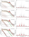 |
Fig. 6 Examples of the smoothed spectrum of KIC6863017 (gray) compared to models that use parameters drawn from the posterior distribution with different numbers of latent parameters. Left column: wide view of the spectrum, showing the background terms, which have the same colorcoding as in Fig. 1, with the combined model samples in red. Right column: zoomed-in view of the p-mode envelope, showing the individual Lorentzian profiles for the modes. |
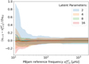 |
Fig. 7 Mode identification precision for a sample of 50 stars using different numbers of latent parameters. The differences between the radial mode frequencies of the PCA method and PBjam are shown in relation to that of δν02 from PBjam. The shaded regions indicate the 68% interval of the observed frequency differences for different numbers of latent parameters used in the model, and the solid colored lines show the median values in each frequency bin. For reference, the dashed line denotes complete agreement between the sets of mode frequencies. |
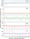 |
Fig. 8 Relative differences of the asymptotic relation parameters determined by PBjam and the PCA method using different numbers of latent parameters. The dashed black lines denote agreement between the two methods. The error bars denote the spread in values for the same sample of 50 stars used in Fig. 7. |
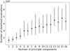 |
Fig. 9 Number of likelihood evaluations needed to reach the nested sampling convergence criteria of Δ log Z ≤ 0.3, for an increasing number of included latent parameters. The error bars indicate the median and 68% percent interval of the distributions for a sample of 50 targets. |
5 Discussion and conclusions
We have presented a method for reducing the complexity of sampling the model parameter space for the asteroseismic analysis of solar-like oscillators. The method uses PCA to define a prior volume in a latent parameter space, which can be more easily sampled than the larger model parameter space.
We tested the PCA method using a spectrum model consisting of three Harvey-like background noise terms, a white noise term, and a series of Lorentzian peaks determined by the asymptotic relation for p modes. This model consists of 16 parameters that are closely related to the physical properties of the star and four parameters that are likely instrument dependent and we therefore left as free variables.
Identifying a single value of the number of latent parameters is likely not possible since our prior sample contains nonlinear correlations over wide ranges of νmax. Furthermore, the density of samples also changes dramatically at ν ≈ 244 μHz since the sample contains observations from both the long- and short-cadence modes of the Kepler mission as well as observations from the TESS mission. We therefore used the effective rank of the covariance matrix and the modified KG criterion to provide an indicator for the choice of the number of latent parameters. Based on these estimates, and the fact that stellar structure and oscillation codes suggest only approximately five dominant fundamental stellar parameters, our expectation is that the number of necessary latent parameters is likely between four and eight for the majority of this particular sample.
From a comparison with reference frequencies and model parameters from PBjam, we find that two latent parameters are, in general, sufficient to produce models that explain the bulk background features of the PSD. This reflects the simple scaling relations for the background model parameters (see, e.g., Kallinger et al. 2014). Using more latent parameters, however, allows the model to more precisely explain the detailed features of the spectrum, such as the mode frequencies. We find that, using more than four latent parameters, the PCA mode frequencies fall within 10% of δν02 of the reference frequencies. Similarly, the majority of the asymptotic model parameters can be recovered to within a few percent by using more than two latent parameters.
This suggests that, for the set of parameters in our prior sample, we are able to reduce the dimensionality of the parameter space by a factor of two to three, and thereby achieve a similar improvement in the time required to sample the posterior distribution. Going forward, this method can be used to add additional terms to the spectrum model, without necessarily increasing the computational complexity. For example, for main-sequence stars the l = 1 and l = 3 modes can likely be added without the need for additional latent parameters since their model parameters are highly correlated with those of the l = 0 and l = 2 modes. For stars evolving off the main sequence, this correlation becomes more complicated due to coupling with buoyancy-dominated modes in the stellar core. Additional latent parameters may therefore be necessary, but the total dimensionality of the sampling will likely still be less than the full model parameter space. This opens the potential for more complicated models to be more rapidly evaluated in a pipeline format, where stellar power density spectra can be analyzed on an ensemble scale.
Acknowledgements
Thanks to Chris Moore for the useful and informative chats. M.B.N. acknowledges support from the UK Space Agency. G.R.D. and W.J.C. acknowledge the support of the UK Science and Technology Facilities Council (STFC). J.O. acknowledges support from NASA through the NASA Hubble Fellowship grant HST-HF2-51517.001 awarded by the Space Telescope Science Institute, which is operated by the Association of Universities for Research in Astronomy, Incorporated, under NASA contract NAS5-26555. This paper has received funding from the European Research Council (ERC) under the European Union’s Horizon 2020 research and innovation programme (CartographY GA. 804752). The authors acknowledge use of the Blue-BEAR HPC service at the University of Birmingham. This paper includes data collected by the Kepler mission and obtained from the MAST data archive at the Space Telescope Science Institute (STScI). Funding for the Kepler mission is provided by the NASA Science Mission Directorate. STScI is operated by the Association of Universities for Research in Astronomy, Inc., under NASA contract NAS5-26555. This paper includes data collected by the TESS mission. Funding for the TESS mission is provided by the NASA’s Science Mission Directorate. This work has made use of data from the European Space Agency (ESA) mission Gaia (https://www.cosmos.esa.int/gaia), processed by the Gaia Data Processing and Analysis Consortium (DPAC, https://www.cosmos.esa.int/web/gaia/dpac/consortium). Funding for the DPAC has been provided by national institutions, in particular the institutions participating in the Gaia Multilateral Agreement. This publication makes use of data products from the Two Micron All Sky Survey, which is a joint project of the University of Massachusetts and the Infrared Processing and Analysis Center/California Institute of Technology, funded by the National Aeronautics and Space Administration and the National Science Foundation.
Appendix A A numerical experiment with stellar models
Here we consider a differential manifold ℳ, admitting an embedding φ: ℳ → ℝN. By the Whitney embedding theorem, such an embedding is guaranteed to exist where N is at least twice the intrinsic dimensionality of ℳ. In the neighborhood of a point p ∈ ℳ described by coordinates {θi: ℳ → ℝ} so that φ(p) = {xj}, the push forward of the tangent vectors to ℳ of these coordinates, { }, have vector components in ℝN that are simply the elements of the Jacobian matrix:
  .
.
In reducing the dimensionality of the mode frequencies, we are implicitly supposing that the set of physically reasonable mode frequencies lie on just such a low-dimensional sub-manifold of what ought to otherwise be nominally a very high-dimensional space, in which any arbitrary set of mode frequencies represents a single point. From the above discussion, to explore the dimensionality of this physically reasonable sub-manifold, we may consider the Jacobian of the mode frequencies (which should collectively be the span of the coordinate basis vectors of the tangent space to this sub-manifold), with respect to a handful of parameters that a priori describe physical changes to the stellar structure (our physically motivated candidate latent variables). These parameters mathematically constitute candidate coordinates on this lower-dimensional manifold.
We computed these Jacobian matrix elements with respect to numerical models of stellar structure constructed using Modules for Experiments in Stellar Astrophysics (MESA; Paxton et al. 2011, 2013, 2015, 2018, 2019) r22.05.1, computing mode frequencies using GYRE (Townsend & Teitler 2013). We considered the following candidate latent variables: (i) R, the stellar radius, (ii) M, the stellar mass, (iii) Yi, the initial helium abundance, (iv) Zi, the initial metal fraction, (v) αMLT, the mixing-length efficiency parameter, and (vi) fov, which describes the scale length of MESA’s implementation of exponential over-mixing.
In addition to these continuous variables, we also consider the following categorical variables: (i) whether or not diffusion and settling of helium and heavy elements was simulated in constructing the stellar models, (ii) which atmospheric boundary condition was applied (Eddington vs. Krishna-Swamy T-τ relations), and (iii) which metal mixture was used (GS98 vs. AGS09).
We first performed this experiment for a solar-calibrated stellar model produced with MESA’s simplex optimization tool, made with element diffusion, a small amount (fov = 0.01) of overshoot, the Eddington T − τ relation, and the GS98 metal mixture. We computed N mode frequencies at l = 0, 1, 2 within ±5∆ν of νmax. In the neighborhood of this reference model, we produce a set of perturbed models, where we perturb each of the continuous variables by 1% relative to their nominal solar-calibrated values. From this perturbation, we are able to evaluate finite-difference derivatives of the mode frequencies with respect to each of these variables. For the categorical variables we only compute simple pairwise differences between identical modes.
We know a priori that the combination M/R3 sets the fundamental frequency of p modes (via ∆ν), so rather than compute the Jacobian with respect to the dimensionful frequencies, we have used instead the Jacobian with respect to ϵ = ν/∆ν − np − l/2. For each variable i that we perturb, the dimensionless differences  form a row of the Jacobian matrix, of shape 9 × N. We then scale each row by its RMS value so that it yields a unit vector in a N-dimensional space: that is to say, we considered only the directions, and not the magnitudes, of the embedded candidate coordinate basis vectors.
Having performed such rescaling, we then used PCA in much the same fashion as we have the observational data. In particular, we considered the eigenvalues from singular value decomposition of the rescaled Jacobian matrix. Since the rescaled Jacobian matrix contains nine unit vectors, its squared eigenvalues should sum to 9. Accordingly, the fractional cumulative sum of squared eigenvalues (ordering the principal components in decreasing rank order) gives us the cumulative explained variance ratio in the mode frequencies induced by changes to this set of latent variables, just as in the case of the scree plot shown in Figure 4 for PCA on observational data.
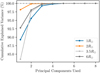 |
Fig. A.1 Cumulative explained variance ratios computed from the singular value decomposition of the Jacobian matrices for dimensionless l = 0, 1, 2 mode frequencies with respect to the nine candidate latent variables described in the main text. Different colors indicate values computed with respect to stellar models at fiducial radii of 1, 2, 3.5, and 6 R⊙. In all other respects, these models are solar-calibrated. Since dimensionless frequencies are used in this calculation, and a combination of M and R sets the fundamental frequency for these normal modes via |

We show this cumulative explained variance ratio for our solar-calibrated model with the blue points in Figure A.1, with N = 30. If the unit vectors that are its rows were all orthogonal, then all of these eigenvalues should be equal to 1, and so this ratio should increase linearly with the number of principal components used. However, we see instead that almost all of the variance can be explained with only two to three of these principal components (i.e., a total of three to four latent variables, once we also account for ∆ν). We repeat this procedure using as fiducial models a few later checkpoints along the solar-calibrated track, at radii of 2, 3.5, and 6 R⊙. For these evolved stellar models, we restrict our attention to l = 0, 2 pure p-mode frequencies (and so have N = 20 in each case), evaluated by the π-mode prescription of Ong & Basu (2020) as implemented in GYRE. These are also shown in Figure A.1 using points and lines of different colors, and behave qualitatively very similarly to the main-sequence case. Thus, at least for pure p modes, only a handful of latent variables is required to describe the collective behavior of a very large number of mode frequencies, even at different stages of stellar evolution.
References
- Appourchaux, T., Chaplin, W. J., García, R. A., et al. 2012, A&A, 543, A54 [CrossRef] [EDP Sciences] [Google Scholar]
- Baglin, A., Miglio, A., Michel, E., & Auvergne, M. 2009, in AIP Conf. Ser., 1170, eds. J.A. Guzik, & P.A. Bradley, 310–314 [NASA ADS] [CrossRef] [Google Scholar]
- Benomar, O., Goupil, M., Belkacem, K., et al. 2018, ApJ, 857, 119 [NASA ADS] [CrossRef] [Google Scholar]
- Borucki, W. J., Koch, D., Basri, G., et al. 2010, Science, 327, 977 [Google Scholar]
- Buchner, J., Georgakakis, A., Nandra, K., et al. 2014, A&A, 564, A125 [NASA ADS] [CrossRef] [EDP Sciences] [Google Scholar]
- Campante, T. L., Corsaro, E., Lund, M. N., et al. 2019, ApJ, 885, 31 [Google Scholar]
- Cangelosi, R., & Goriely, A. 2007, Biol. Direct, 2, 2 [CrossRef] [Google Scholar]
- Chaplin, W. J. & Miglio, A. 2013, ARA&A, 51, 353 [NASA ADS] [CrossRef] [Google Scholar]
- Chaplin, W. J., Kjeldsen, H., Bedding, T. R., et al. 2011, ApJ, 732, 54 [CrossRef] [Google Scholar]
- Chaplin, W. J., Basu, S., Huber, D., et al. 2014, ApJS, 210, 1 [Google Scholar]
- Chontos, A., Huber, D., Berger, T. A., et al. 2021, Apj, 922, 229 [CrossRef] [Google Scholar]
- Corsaro, E., McKeever, J. M., & Kuszlewicz, J. S. 2020, A&A, 640, A130 [NASA ADS] [CrossRef] [EDP Sciences] [Google Scholar]
- Cunha, M.S., Roxburgh, I. W., Aguirre Børsen-Koch, V., et al. 2021, MNRAS, 508, 5864 [NASA ADS] [CrossRef] [Google Scholar]
- Davies, G. R., Silva Aguirre, V., Bedding, T. R., et al. 2016, MNRAS, 456, 2183 [Google Scholar]
- Duvall, T.L.Jr., & Harvey, J.W. 1986, in NATO Advanced Science Institutes (ASI) Series C, 169, NATO Advanced Science Institutes (ASI) Series C, ed. D.O. Gough (D. Reidel Publishing Company), 105 [Google Scholar]
- Evans, D. W., Riello, M., De Angeli, F., et al. 2018, A&A, 616, A4 [NASA ADS] [CrossRef] [EDP Sciences] [Google Scholar]
- Goodfellow, I., Bengio, Y., & Courville, A. 2016, Deep Learning (MIT Press), http://www.deeplearningbook.org [Google Scholar]
- Guttman, L. 1954, Psychometrika, 19, 149 [Google Scholar]
- Guyon, I., & Elisseeff, A. 2003, J. Mach. Learn. Res., 3, 1157 [Google Scholar]
- Hall, O. J., Davies, G. R., van Saders, J., et al. 2021, Nat. Astron., 5, 707 [NASA ADS] [CrossRef] [Google Scholar]
- Handberg, R., & Campante, T. L. 2011, A&A, 527, A56 [CrossRef] [EDP Sciences] [Google Scholar]
- Harris, C. R., Millman, K. J., van der Walt, S.J., et al. 2020, Nature, 585, 357 [NASA ADS] [CrossRef] [Google Scholar]
- Harvey, J. 1985, in ESA SP, 235, eds. E. Rolfe, & B. Battrick, 199 [Google Scholar]
- Hatt, E., Nielsen, M. B., Chaplin, W. J., et al. 2023, A&A, 669, A67 [NASA ADS] [CrossRef] [EDP Sciences] [Google Scholar]
- Hon, M., Stello, D., García, R. A., et al. 2019, MNRAS, 485, 5616 [NASA ADS] [Google Scholar]
- Huber, D., Bedding, T. R., Stello, D., et al. 2011, ApJ, 743, 143 [Google Scholar]
- Jolliffe, I. T. 1972, J. Roy. Stat. Soc. Ser. C (Appl. Stat.), 21, 160 [Google Scholar]
- Kaiser, H. F. 1960, Educ. Psychol. Meas., 20, 141 [Google Scholar]
- Kallinger, T., De Ridder, J., Hekker, S., et al. 2014, A&A, 570, A41 [NASA ADS] [CrossRef] [EDP Sciences] [Google Scholar]
- Kingma, D. P., & Welling, M. 2013, ArXiv e-prints [arXiv:1312.6114] [Google Scholar]
- Kjeldsen, H., & Bedding, T. R. 1995, A&A, 293, 87 [NASA ADS] [Google Scholar]
- Kjeldsen, H., & Bedding, T. R. 2011, A&A, 529, A8 [NASA ADS] [CrossRef] [EDP Sciences] [Google Scholar]
- Lebreton, Y., & Goupil, M. J. 2014, A&A, 569, A21 [NASA ADS] [CrossRef] [EDP Sciences] [Google Scholar]
- Lee, D. D., & Seung, H. S. 1999, Nature, 401, 788 [Google Scholar]
- Li, T., Li, Y., Bi, S., et al. 2022, ApJ, 927, 167 [NASA ADS] [CrossRef] [Google Scholar]
- Lund, M. N., Silva Aguirre, V., Davies, G. R., et al. 2017, ApJ, 835, 172 [Google Scholar]
- Mosser, B., Vrard, M., Belkacem, K., Deheuvels, S., & Goupil, M. J. 2015, A&A, 584, A50 [NASA ADS] [CrossRef] [EDP Sciences] [Google Scholar]
- Nielsen, M. B., Davies, G. R., Ball, W. H., et al. 2021, AJ, 161, 62 [NASA ADS] [CrossRef] [Google Scholar]
- Ong, J. M. J., & Basu, S. 2020, ApJ, 898, 127 [NASA ADS] [CrossRef] [Google Scholar]
- Paxton, B., Bildsten, L., Dotter, A., et al. 2011, ApJS, 192, 3 [Google Scholar]
- Paxton, B., Cantiello, M., Arras, P., et al. 2013, ApJS, 208, 4 [Google Scholar]
- Paxton, B., Marchant, P., Schwab, J., et al. 2015, ApJS, 220, 15 [Google Scholar]
- Paxton, B., Schwab, J., Bauer, E. B., et al. 2018, ApJS, 234, 34 [NASA ADS] [CrossRef] [Google Scholar]
- Paxton, B., Smolec, R., Schwab, J., et al. 2019, ApJS, 243, 10 [Google Scholar]
- Ricker, G. R., Winn, J. N., Vanderspek, R., et al. 2015, J. Astron. Telescopes Instrum. Syst., 1, 014003 [Google Scholar]
- Roy, O., & Vetterli, M. 2007, in 2007 15th European Signal Processing Conference, 606 [Google Scholar]
- Shannon, C. E. 1948, Bell Syst. Tech. J., 27, 379 [Google Scholar]
- Silva Aguirre, V., Lund, M. N., Antia, H. M., et al. 2017, ApJ, 835, 173 [Google Scholar]
- Skilling, J. 2004, in AIP Conf. Ser., 735, Bayesian Inference and Maximum Entropy Methods in Science and Engineering: 24th International Workshop on Bayesian Inference and Maximum Entropy Methods in Science and Engineering, eds. R. Fischer, R. Preuss, & U.V. Toussaint, 395 [NASA ADS] [CrossRef] [Google Scholar]
- Speagle, J. S. 2020, MNRAS, 493, 3132 [Google Scholar]
- Tamuz, O., Mazeh, T., & Zucker, S. 2005, MNRAS, 356, 1466 [Google Scholar]
- Townsend, R. H. D., & Teitler, S. A. 2013, MNRAS, 435, 3406 [Google Scholar]
- Viani, L. S., Basu, S., Chaplin, W. J., Davies, G. R., & Elsworth, Y. 2017, ApJ, 843, 11 [NASA ADS] [CrossRef] [Google Scholar]
- White, T. R., Bedding, T. R., Gruberbauer, M., et al. 2012, ApJ, 751, L36 [NASA ADS] [CrossRef] [Google Scholar]
- Woodard, M. F. 1984, PhD thesis, University of California, San Diego, USA [Google Scholar]
- Yu, J., Huber, D., Bedding, T. R., et al. 2018, ApJS, 236, 42 [NASA ADS] [CrossRef] [Google Scholar]
In our case, when each model parameter is normalized to unit variance, and with weights wn = 1, the covariance and correlation matrices are identical.
All Tables
All Figures
|
Fig. 1 Example spectrum of the red giant ϵ Reticuli. The PSD is shown in light and dark gray (smoothed). The components of the background model are shown with dashed lines, while the combined spectrum model, including the mode components, is shown in red. The parameters of the spectrum model are drawn from the prior sample around νmax ≈ 300 μHz the equivalent to that of ϵ Reticuli. |
| In the text | |
|
Fig. 2 ϵ and log νmax values for a selection of the K = 10 (green) and K = 200 (orange) nearest neighbors, determined by the Euclidean distance relative to an example target with a notional νmax ≈ 830 μHz (horizontal purple line), an effective temperature Teff ≈ 5640 K, and GBP − GRP ≈ 0.86. |
| In the text | |
|
Fig. 3 Corner plots of a sample of 400 targets around νmax = 100 μHz drawn from the prior distribution. Left: projection of the sample into the latent parameter space (in black) and a corresponding sample (in blue) drawn from the one-dimensional KDE approximations of the marginalized distributions (diagonal frames). Right: original 400 prior sample draws (in black) with the sample drawn from the latent space, projected into the model parameter space (in blue). For clarity we only show a subset of the model parameters, where all parameters except ε are in base-10 logarithmic units. |
| In the text | |
|
Fig. 4 Eigenvalues of a covariance matrix computed from 400 samples of θ around and input νmax = 100 μHz where θ consists of 16 parameters. The eigenvalues are ordered by descending value, and the first few corresponding eigenvectors explain the majority of the sample variance. |
| In the text | |
|
Fig. 5 Cumulative explained variance of 400 samples of θ for different combinations of input νmax and selected eigenvectors. The dashed line indicates the delineation between stars observed in Kepler long cadence (low frequency) and short cadence (high frequency). The effective covariance matrix rank is indicated in red, and the number of latent parameters suggested by Jolliffe’s modified KG criterion is shown in purple. |
| In the text | |
|
Fig. 6 Examples of the smoothed spectrum of KIC6863017 (gray) compared to models that use parameters drawn from the posterior distribution with different numbers of latent parameters. Left column: wide view of the spectrum, showing the background terms, which have the same colorcoding as in Fig. 1, with the combined model samples in red. Right column: zoomed-in view of the p-mode envelope, showing the individual Lorentzian profiles for the modes. |
| In the text | |
|
Fig. 7 Mode identification precision for a sample of 50 stars using different numbers of latent parameters. The differences between the radial mode frequencies of the PCA method and PBjam are shown in relation to that of δν02 from PBjam. The shaded regions indicate the 68% interval of the observed frequency differences for different numbers of latent parameters used in the model, and the solid colored lines show the median values in each frequency bin. For reference, the dashed line denotes complete agreement between the sets of mode frequencies. |
| In the text | |
|
Fig. 8 Relative differences of the asymptotic relation parameters determined by PBjam and the PCA method using different numbers of latent parameters. The dashed black lines denote agreement between the two methods. The error bars denote the spread in values for the same sample of 50 stars used in Fig. 7. |
| In the text | |
|
Fig. 9 Number of likelihood evaluations needed to reach the nested sampling convergence criteria of Δ log Z ≤ 0.3, for an increasing number of included latent parameters. The error bars indicate the median and 68% percent interval of the distributions for a sample of 50 targets. |
| In the text | |
|
Fig. A.1 Cumulative explained variance ratios computed from the singular value decomposition of the Jacobian matrices for dimensionless l = 0, 1, 2 mode frequencies with respect to the nine candidate latent variables described in the main text. Different colors indicate values computed with respect to stellar models at fiducial radii of 1, 2, 3.5, and 6 R⊙. In all other respects, these models are solar-calibrated. Since dimensionless frequencies are used in this calculation, and a combination of M and R sets the fundamental frequency for these normal modes via |
| In the text | |
Current usage metrics show cumulative count of Article Views (full-text article views including HTML views, PDF and ePub downloads, according to the available data) and Abstracts Views on Vision4Press platform.
Data correspond to usage on the plateform after 2015. The current usage metrics is available 48-96 hours after online publication and is updated daily on week days.
Initial download of the metrics may take a while.