| Issue |
A&A
Volume 675, July 2023
|
|
|---|---|---|
| Article Number | L1 | |
| Number of page(s) | 11 | |
| Section | Letters to the Editor | |
| DOI | https://doi.org/10.1051/0004-6361/202346305 | |
| Published online | 30 June 2023 | |
Letter to the Editor
Dynamical detection of a companion driving a spiral arm in a protoplanetary disk⋆
1
Aix Marseille Univ, CNRS, CNES, LAM, Marseille, France
e-mail: This email address is being protected from spambots. You need JavaScript enabled to view it.
2
Université Côte d’Azur, Observatoire de la Côte d’Azur, CNRS, Laboratoire Lagrange, Bd de l’Observatoire, CS 34229, 06304 Nice Cedex 4, France
3
Université Grenoble Alpes, CNRS, Institut de Planétologie et d’Astrophysique (IPAG), 38000 Grenoble, France
4
Department of Physics & Astronomy, University of Victoria, Victoria, BC, V8P 5C2
Canada
5
Univ Lyon, Univ Claude Bernard Lyon 1, ENS de Lyon, CNRS, Centre de Recherche Astrophysique de Lyon UMR5574, 69230 Saint-Genis-Laval, France
6
Steward Observatory, University of Arizona, Tucson, AZ, USA
7
Department of Astronomy, Xiamen University, 1 Zengcuoan West Road, Xiamen, Fujian, 361005
PR China
8
Dipartimento di Fisica, Università degli Studi di Milano, Via Celoria 16, 20133 Milano, MI, Italy
Received:
2
March
2023
Accepted:
14
June
2023
Abstract
Radio and near-infrared observations have observed dozens of protoplanetary disks that host spiral arm features. Numerical simulations have shown that companions may excite spiral density waves in protoplanetary disks via companion–disk interaction. However, the lack of direct observational evidence for spiral-driving companions poses challenges to current theories of companion–disk interaction. Here we report multi-epoch observations of the binary system HD 100453 with the Spectro-Polarimetric High-contrast Exoplanet REsearch (SPHERE) facility at the Very Large Telescope. By recovering the spiral features via robustly removing starlight contamination, we measure spiral motion across 4 yr to perform dynamical motion analyses. The spiral pattern motion is consistent with the orbital motion of the eccentric companion. With this first observational evidence of a companion driving a spiral arm among protoplanetary disks, we directly and dynamically confirm the long-standing theory on the origin of spiral features in protoplanetary disks. With the pattern motion of companion-driven spirals being independent of companion mass, here we establish a feasible way of searching for hidden spiral-arm-driving planets that are beyond the detection of existing ground-based high-contrast imagers.
Key words: planet-disk interactions / protoplanetary disks / techniques: high angular resolution / techniques: image processing / stars: individual: HD 100453
FITS images are only available at the CDS via anonymous ftp to cdsarc.cds.unistra.fr (130.79.128.5>) or via https://cdsarc.cds.unistra.fr/viz-bin/cat/J/A+A/675/L1
Marie Skłodowska-Curie Fellow.
© The Authors 2023
 Open Access article, published by EDP Sciences, under the terms of the Creative Commons Attribution License (https://creativecommons.org/licenses/by/4.0), which permits unrestricted use, distribution, and reproduction in any medium, provided the original work is properly cited.
This article is published in open access under the Subscribe to Open model. This email address is being protected from spambots. You need JavaScript enabled to view it. to support open access publication.
1. Introduction
The detection of spiral structures in protoplanetary disks has called for the understanding of spiral formation mechanisms (Dong et al. 2018). Theoretical and hydrodynamical simulation studies have suggested that companion–disk interaction and disk gravitational instability (GI), together with other mechanisms such as vortex and shadowing (e.g., Marr & Dong 2022; Montesinos et al. 2016), are the most compelling ways to explain the origin of spirals. To test spiral formation mechanisms, hydrodynamical simulations (e.g., Dong et al. 2016b; Meru et al. 2017; Hall et al. 2018) and multi-epoch imaging studies (e.g., Ren et al. 2020a; Boccaletti et al. 2021; Xie et al. 2021; Safonov et al. 2022) have been employed to associate spiral configuration or motion with the formation mechanism.
Although motion studies can distinguish theoretical mechanisms between companion-driven and GI-induction, there has been no observationally direct dynamical evidence of the co-motion of a companion and the spiral that it drives. This calls for the verification of the basic assumption in associating the companion–disk interaction theory with spiral motion: the co-motion of companion and spiral (e.g., Ren et al. 2018a). It is thus of importance to push beyond identifying companions in spiral systems (e.g., Currie et al. 2022) by directly validating the motion measurement approach. Therefore, we need to apply motion studies to spiral systems with known companion(s).
In addition to validating the formation and motion mechanism of companion-driven spirals, an application to the known companion–spiral system(s) can also formally establish the existence of these currently hidden spiral-driving planets, especially since such planets are the most compelling targets for confirmation with direct imaging using state-of-the-art telescopes (e.g., VLT/ERIS, JWST) in this current era where targeted imaging approaches (e.g., Bohn et al. 2020; Currie et al. 2023; Franson et al. 2023; De Rosa et al. 2023; Mesa et al. 2023) instead of blind search are necessary to efficiently populate the family of directly imaged exoplanets. To establish the motion pattern in systems with known spirals and companions, multi-epoch imaging using identical instrument and observation modes can be ideal for minimizing instrument differences and data reduction bias.
HD 100453 is a binary system (Chen et al. 2006) at a distance of 103.8 ± 0.2 pc (Gaia Collaboration 2023) with an age of 6.5 ± 0.5 Myr (Vioque et al. 2018). The primary star HD 100453 A (hereafter HD 100453) is a young Herbig A9Ve star with a mass of 1.70 ± 0.09 M⊙ (Dominik et al. 2003). The protoplanetary disk around the primary star was directly imaged at near-infrared (NIR) and submillimeter wavelengths, showing a cavity, a ring, and two spiral arms from inside out (Benisty et al. 2017; Wagner et al. 2018; van der Plas et al. 2019; Rosotti et al. 2020). NIR interferometric observations revealed the presence of the inner disk (Menu et al. 2015; Kluska et al. 2020; Bohn et al. 2022) inside the cavity that is misaligned with and shadows the outer spiral disk (Bohn et al. 2022; Benisty et al. 2017).
The secondary star HD 100453 B (hereafter the companion) is an early M star with a mass of 0.2 ± 0.04 M⊙ (Collins et al. 2009), located at a projected distance of around 1.05″ (109 au). The HD 100453 system offers a particularly decisive test of co-motion between spirals and companions that might be driving them. Numerical simulations suggest that such a companion can truncate the disk and excite two spiral arms in the remaining disk as observed in the NIR (Dong et al. 2016b). The companion-driven origin of the spiral arms was supported by one of the observed spiral arms in the 12CO line that connects to the companion position by assuming a coplanar orbit (Rosotti et al. 2020). However, the potential mutual inclination between the companion orbit and the spiral disk (van der Plas et al. 2019; Gonzalez et al. 2020) raised the possibility of a projection effect. With HD 100453 being the exemplary configuration of a companion–spiral system, we study the motions of the spiral(s) and the companion here.
2. Observations and data reduction
The HD 100453 system was observed with the Spectro-Polarimetric High-contrast Exoplanet REsearch (SPHERE; Beuzit et al. 2019) instrument at the Very Large Telescope (VLT) using the InfraRed Dual-band Imager and Spectrograph (IRDIS; Dohlen et al. 2008). For spiral motion analysis, we retrieved three total intensity observations in K1-band (λ = 2.11 μm and Δλ = 0.10 μm) in April 2015 and April 2019, with a time span of 4.0 years. The observation and the pre-processing of the data are summarized in Appendix A. Throughout the paper the observation of the disk on 08 April 2019 is only used for uncertainty estimation because its integration time is shorter than the observation on 07 April 2019 (see Table A.1).
We processed the calibrated data by applying reference-star differential imaging (RDI) using the reference images assembled from Xie et al. (2022). We constructed a coronagraphic model of stellar signals and speckles via data imputation using sequential nonnegative matrix factorization (DI-sNMF; Ren et al. 2020b) (see Appendix B for a description of the detailed procedures). Combining the two techniques, RDI-DIsNMF is optimized for the direct imaging of circumstellar disks in total intensity by minimizing self-subtraction and overfitting that has plagued previous methods. We first generated the speckle features (i.e., NMF components of the stellar coronagraphic model) based on the disk-free reference library from Xie et al. (2022) using NMF from Ren et al. (2018b), then used these features to remove the speckles in HD 100453 observations.
To avoid the overfitting problem for RDI (e.g., Soummer et al. 2012; Pueyo 2016) that can change the morphology of spirals and bias spiral motion measurement, we masked out regions that host disk signals in HD 100453 data, and modeled the rest of the region using the NMF components, and then imputed the signals in disk hosting regions (Ren et al. 2020b). With RDI-DIsNMF using well-chosen reference images, we were able to accurately recover the disk morphology with theoretically minimum post-processing artifacts, which is an essential requirement for accurate measurement of the pattern motion of spiral features.
3. Dynamical analysis
3.1. Pattern motion of the spiral arm S1
Using RDI-DIsNMF, we recovered the disk around HD 100453 at 2.11 μm in total intensity (Fig. 1). The disk morphology is consistent with that in the polarimetric image (Benisty et al. 2017). In particular, we confidently recovered two spiral arms, S1 and S2. S1 is the primary arm that has CO gas connected to the projected position of the companion (Rosotti et al. 2020). To measure the positions of the spiral arms, we first needed to correct the viewing geometry. We deprojected each disk image to face-on views (i.e., the disk plane) adopting an inclination of  and a position angle (PA) of
  (Bohn et al. 2022). To correct for disk flaring, we assumed that the disk scale height (h) follows h = 0.22 × r1.04, where r is radial separation in au (Benisty et al. 2017). Each disk image was then r2-scaled to enhance the disk features at large radii. Finally, we transformed them into polar coordinates for the measurement of spiral arm locations. We determined the local maxima of the arm at each azimuthal angle in 1° steps by performing Gaussian profile fitting (see Appendix C for a detailed description).
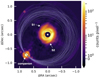 |
Fig. 1. SPHERE/IRDIS detection of the HD 100453 system in K1, showing the companion and two spiral arms around a ring-like structure. The gray lines represent the companion orbits that can dynamically drive the spiral arm. The white star shows the position of the primary star. |
The local maxima of spiral arm S1 are presented in Fig. 2, which describes the morphology of S1. An offset over a large range of 210°–260° is visible between the two epochs of 2015 and 2019, and follows the rotational direction of the disk. This offset also appears when simply comparing disk images between 2015 and 2019 (see Fig. B.1). At locations < 210° we are limited by the signal-to-noise ratio (S/N) of the disk where the spiral arm is barely detected. At locations > 260°, the spiral arm starts to merge with the ring-like structure, which increases the uncertainty of the local maxima of the spiral arm. Because possible systematics such as the image misalignment caused by the instrument have been properly corrected during the image alignment (Appendix A), we conclude that the offset is caused by the pattern motion of the S1 arm in 2015–2019.
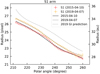 |
Fig. 2. Peak locations of spiral arm S1 in polar coordinates after correction for viewing geometry. The solid curves represent the best-fit model spiral for the peak locations (dot points) between 2015 and 2019, assuming the companion-driven scenario. The derived angular velocities of spiral pattern motion are |

Following Ren et al. (2020a), we fitted five-degree polynomials to the spiral arm S1 in two epochs and simultaneously obtain their morphological parameters and the pattern motion of the spiral arms. The fitting result is shown in Fig. 2. In principle, different parts of the spiral have different pattern speeds if driven by a companion on an eccentric orbit. However, our data do not permit a radius-dependent assessment, and a single-value pattern speed is measured as a compromise. The speed of the pattern motion for spiral arm S1 is  yr−1 in the counterclockwise direction, assuming the companion-driven scenario that the pattern speed is a constant for S1. The uncertainty estimation is described in Appendix D. The deprojection will affect the spiral location determination, and subsequently the spiral motion measurement. However, the disk flaring of HD 100453 only has limited impact on the velocity of the spiral motion (see Appendix E). Throughout the paper we present the velocity of the spiral motion based on the best-fit model (h = 0.22 × r1.04) from Benisty et al. (2017) to correct for the disk flaring in the deprojection.
We examined the possibility of the gravitational instability (GI) scenario that each part of the arms rotates at its local Keplerian motion. Based on the fitted morphological parameters of the S1 arm in 2015, we predicted the location of the S1 arm in 2019, and adopted the stellar mass of 1.7 M⊙ for the central star. The predicted locations of GI-induced spiral arms deviate from the observed arm locations in 2019 (Fig. 2). The local Keplerian motions at 25 to 35 au are  yr−1 to
  yr−1, or
  to
to  in 4 yr. The local Keplerian motions are too large to explain the observation (∼3.5° in 4 years). We conclude that the spiral arm S1 is not triggered by gravitational instability. Together with MWC 758 (Ren et al. 2020a) and SAO 206462 (Xie et al. 2021), HD 100453 is the third spiral disk that disfavors the GI origin for their spirals from pattern motion measurement.
3.2. Motion of the stellar companion
The companion HD 100453 B has over 15 years of astrometric data. We adopt astrometric data from Collins et al. (2009), Wagner et al. (2018), and Gonzalez et al. (2020) (see Table F.1). A linear fit to the PAs of the companion shows that the companion has an angular velocity of  yr−1 in the sky plane between 2003 and 2019 (Appendix F). Based on the PAs only in 2015 and 2019, we also obtain an angular velocity of
  yr−1 for the companion, which is consistent with our linear fit. Hence, we adopt the fitting result as the angular velocity of the companion because it contains more independent measurements. To obtain the companion motion in the disk plane, we deprojected the angular velocity of the companion from the sky plane to the disk plane. In the deprojection, we adopt the disk inclination, the disk position angle, and the companion position angle to be
  ,
,  , and
, and  , respectively. We obtain the angular velocity of the companion in the disk plane to be
  yr−1 between 2015 and 2019.
We also estimate the probability density distribution of the companion angular velocity in the disk plane (Appendix G). We calculate the companion angular velocity based on the companion orbital parameters adopted from the orbit fitting results in Gonzalez et al. (2020). The derived probability density distribution has a Gaussian profile; the companion has an angular velocity of  yr−1 (1σ credible interval) in the disk plane in 2019. The angular velocity derived from the orbital parameters is consistent with the direct linear fit to the companion PAs. This consistent angular velocity and its Gaussian distribution are expected because the companion motion between 2003 and 2019 is well constrained by the astrometry data with the measuring uncertainty followed potential Gaussian noise.
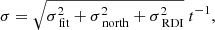
In general, the spiral pattern motion should be in the range of the slowest and fastest companion orbital frequency in the scenario of an eccentric perturber (see Eq. (12) in Zhu & Zhang 2022). From the posterior probability distribution of the orbital parameters obtained by Gonzalez et al. (2020), we derived the minimum and maximum value of the companion orbital motion. Although the companion motion at the location in 2019 is slower than the spiral motion in 2019, the maximum value of the companion orbital motion is still larger than the measured spiral motion (see Fig. 3). It suggests that the physical interaction (i.e., tidal interaction) between the companion and the disk can exist, as proposed by the numerical simulation in Dong et al. (2016b).
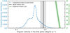 |
Fig. 3. Angular velocity of the S1 spiral pattern motion in HD 100453 (black line). It could follow local Keplerian motion (green curve) or be smaller than the maximum value of the companion orbital motion (blue curve), under gravitational instability (GI) or companion–disk interaction, respectively. The measured spiral motion is consistent with the companion motion in the system and is inconsistent with the local Keplerian motion, revealing the companion-driven origin of the spiral arm S1, while excluding the GI origin. The motions here adopt a central stellar mass of 1.70 ± 0.09 M⊙. The colored shaded regions around each curve represent the corresponding uncertainties. |
Based on the consistency in motion measurements, we conclude that the known companion HD 100453 B drives the spiral arm S1. This is the first detection of a companion driving a spiral arm among protoplanetary disks. In light of our result, the previously observed CO gas extending from the S1 arm in Rosotti et al. (2020) is also dynamically connected to the companion, rather than moving independently, and the static connection arises from projection effects due to the relative inclination between the disk and the companion orbit.
4. Discussion
4.1. Pattern motion of the spiral arm S2
HD 100453 was classified as a Group I disk that has an outer disk flaring (Meeus et al. 2001). The bottom of the S2 spiral arm shown in the NIR polarimetric image suggests the disk thickness is nonnegligible and the S2 arm locates on the near side of the disk (Benisty et al. 2017). NIR observations probe the scattered light from the disk surface. For the disk with flaring, the angle between the disk surface on the nearside of the disk (i.e., S2) and the sky plane is larger than the disk inclination of  . We define the disk inclination to be the angle between the flat disk midplane and the sky plane. Large viewing angles (i.e.,
  ) prevent us from restoring the correct face-on morphology via the deprojection (Dong et al. 2016a). Unlike S2, S1 locates on the far side of the disk where the inclination of the disk surface is smaller than the disk inclination. Thus, it is more accurate to restore the S1 arm back to face-on morphology than the S2 arm. Therefore, we did not provide a motion measurement for the S2 arm.
4.2. Other spiral-triggering mechanisms
Spiral features can also be induced by a flyby (Ménard et al. 2020; Dong et al. 2022). However, a recent search for potential stellar flybys with Gaia DR3 did not identify recent close-in on-sky flyby candidates around HD 100453 (Shuai et al. 2022). Thus, this scenario is unlikely to cause the spiral feature in this system.
The disk of HD 100453 seen in the NIR contains two shadows (Fig. 1) created by the inner disk (Bohn et al. 2022). Benisty et al. (2017) explored the possibility of the shadow-triggered spirals via the pressure decrease (Montesinos et al. 2016). However, spiral arms triggered by shadows should follow the local Keplerian motion as GI-induced spirals. Therefore, we excluded the shadows being the origin of the spiral features in HD 100453.
4.3. Feasibility of locating spiral-driving planets
In protoplanetary and transitional disks, the occurrence rate and orbital distribution of the embedded planet population remain to be established due to a limited number of confirmed proto-planets. The current high-contrast imagers with low spectrum resolution (i.e., R < 100) at NIR wavelengths cannot easily discriminate between the scattered light from the dusty disk and that of the embedded planet (Rameau et al. 2017; Currie et al. 2019; Rich et al. 2019). Hα surveys for the signal of planetary accretions mostly resulted in nondetections of planets (Cugno et al. 2019; Zurlo et al. 2020; Xie et al. 2020), possibly caused by high extinction or periodic accretions if the forming planet is present. In summary, current instruments with conventional techniques are inefficient in the search for planets embedded in disks.
Our dynamical motion analysis of the HD 100453 system validated the approach of mapping spiral arm motion to locate hidden giant planets in protoplanetary disks, first proposed by Ren et al. (2020a). Although we only investigated a nonplanetary companion in this specific study, the pattern speed of companion-driven spirals depends on the location of the companion instead of its mass. Furthermore, the sensitivity of our motion measurement directly depends on the time span (see Eq. (D.1)). The uncertainty of the motion measurement decreases with the increase in the time span (t) of two epochs. Typical 1σ uncertainties for the motion measurements based on two epochs (if t = 5 yr) of SPHERE observations in total intensity and polarized light are about  yr−1 (Appendix D) and
  yr−1 (Ren et al. 2020a), respectively. Therefore, spiral motions driven by a planet can be detected and distinguished from local Keplerian motions (GI scenario) within a feasible time of a few years.
From the posterior probability distribution of orbital parameters obtained by Gonzalez et al. (2020), we derived the companion orbits that can dynamically drive the spiral arm (see Fig. 1). The corresponding probability distribution of orbital parameters is shown in Fig. H.1. Our dynamical analysis opens a new and feasible window to probe the orbit distribution of planets in the spiral disks that currently are difficult to study via conventional techniques of direct imaging and spectroscopy. The measured spiral motion can determine the range of the planet eccentricity (e.g., Eq. (12) in Zhu & Zhang 2022). In combination with the planet mass estimated from the morphology of the spiral arms (Fung & Dong 2015) or simply using mass upper limits from direct imaging, we can infer the formation and migration of planets at the early stage.
5. Conclusion
We present multi-epoch observations of the HD 100453 system and perform a dynamical analysis for the spiral motion in 4 yr. The measured pattern motion of the spiral arm S1 disfavors the GI origin. More importantly, the orbital motion of companion HD 100453 B can explain the spiral pattern motion in the scenario of the eccentric perturber. It is the first dynamical detection of a companion driving a spiral arm among protoplanetary disks.
Companion–disk interaction is a long-standing theory that could naturally explain the origin of spiral features in disks. For the first time, our dynamical analyses directly confirm that the companion–disk interaction can indeed induce spiral arms in disks, supporting that it could also be the formation mechanism for other spiral systems without detected companions. Our dynamical detection also validates our method to be a feasible way of searching for and locating hidden spiral-arm-driving planets that are best targets for dedicated direct imaging explorations (e.g., Bae et al. 2022, Fig. 7 therein) with upcoming state-of-the-art high-contrast imagers.
https://github.com/avigan/SPHERE, version 1.4.2
Acknowledgments
We thank Dr. Faustine Cantalloube for the beneficial discussion about the low wind effect. The disk images of HD 100453 are based on observations collected at the European Organisation for Astronomical Research in the Southern Hemisphere under ESO programmes 095.C-0389(A) and 0103.C-0847(A). We thank all the principal investigators and their collaborators who prepared and performed the observations with SPHERE. Without their efforts, we would not be able to build the master reference library to enable our RDI technique. B.B.R. acknowledges funding from the European Research Council (ERC) under the European Union’s Horizon 2020 research and innovation programme (grant PROTOPLANETS No. 101002188), and from the European Union’s Horizon 2020 research and innovation programme under the Marie Skłodowska-Curie grant agreement No. 101103114. R.D. acknowledges financial support provided by the Natural Sciences and Engineering Research Council of Canada through a Discovery Grant, as well as the Alfred P. Sloan Foundation through a Sloan Research Fellowship. E.C. acknowledges funding from the European Research Council (ERC) under the European Union’s Horizon Europe research and innovation programme (ESCAPE, grant agreement No 101044152). A.V. acknowledges funding from the European Research Council (ERC) under the European Union’s Horizon 2020 research and innovation programme (grant agreement No. 757561). J.-F.G. acknowledges funding from the European Union’s Horizon 2020 research and innovation programme under the Marie Skłodowska-Curie grant agreement No 823823 (DUSTBUSTERS) and from the ANR (Agence Nationale de la Recherche) of France under contract number ANR-16- CE31-0013 (Planet-Forming-Disks), and thanks the LABEX Lyon Institute of Origins (ANR-10-LABX-0066) for its financial support within the Plan France 2030 of the French government operated by the ANR. T.F. acknowledges supports from the National Key R&D Program of China No. 2017YFA0402600, from NSFC grants No. 11890692, 12133008, and 12221003, and from the science research grants from the China Manned Space Project with No. CMS-CSST-2021-A04.
References
- Bae, J., Isella, A., Zhu, Z., et al. 2022, ArXiv e-prints [arXiv:2210.13314] [Google Scholar]
- Benisty, M., Stolker, T., Pohl, A., et al. 2017, A&A, 597, A42 [NASA ADS] [CrossRef] [EDP Sciences] [Google Scholar]
- Beuzit, J. L., Vigan, A., Mouillet, D., et al. 2019, A&A, 631, A155 [NASA ADS] [CrossRef] [EDP Sciences] [Google Scholar]
- Blunt, S., Nielsen, E. L., De Rosa, R. J., et al. 2017, AJ, 153, 229 [Google Scholar]
- Blunt, S., Wang, J. J., Angelo, I., et al. 2020, AJ, 159, 89 [NASA ADS] [CrossRef] [Google Scholar]
- Boccaletti, A., Pantin, E., Ménard, F., et al. 2021, A&A, 652, L8 [NASA ADS] [CrossRef] [EDP Sciences] [Google Scholar]
- Bohn, A. J., Kenworthy, M. A., Ginski, C., et al. 2020, MNRAS, 492, 431 [Google Scholar]
- Bohn, A. J., Benisty, M., Perraut, K., et al. 2022, A&A, 658, A183 [NASA ADS] [CrossRef] [EDP Sciences] [Google Scholar]
- Cantalloube, F., Farley, O. J. D., Milli, J., et al. 2020, A&A, 638, A98 [NASA ADS] [CrossRef] [EDP Sciences] [Google Scholar]
- Carbillet, M., Bendjoya, P., Abe, L., et al. 2011, Exp. Astron., 30, 39 [Google Scholar]
- Chauvin, G., Lagrange, A. M., Bonavita, M., et al. 2010, A&A, 509, A52 [NASA ADS] [CrossRef] [EDP Sciences] [Google Scholar]
- Chen, X. P., Henning, T., van Boekel, R., & Grady, C. A. 2006, A&A, 445, 331 [NASA ADS] [CrossRef] [EDP Sciences] [Google Scholar]
- Collins, K. A., Grady, C. A., Hamaguchi, K., et al. 2009, ApJ, 697, 557 [NASA ADS] [CrossRef] [Google Scholar]
- Cugno, G., Quanz, S. P., Hunziker, S., et al. 2019, A&A, 622, A156 [NASA ADS] [CrossRef] [EDP Sciences] [Google Scholar]
- Currie, T., Marois, C., Cieza, L., et al. 2019, ApJ, 877, L3 [Google Scholar]
- Currie, T., Lawson, K., Schneider, G., et al. 2022, Nat. Astron., 6, 751 [NASA ADS] [CrossRef] [Google Scholar]
- Currie, T., Brandt, G. M., Brandt, T. D., et al. 2023, Science, 380, 198 [NASA ADS] [CrossRef] [Google Scholar]
- De Rosa, R. J., Nielsen, E. L., Wahhaj, Z., et al. 2023, A&A, 672, A94 [NASA ADS] [CrossRef] [EDP Sciences] [Google Scholar]
- Dohlen, K., Langlois, M., Saisse, M., et al. 2008, in Ground-based and Airborne Instrumentation for Astronomy II, eds. I. S. McLean, & M. M. Casali, SPIE Conf. Ser., 7014, 70143L [NASA ADS] [Google Scholar]
- Dominik, C., Dullemond, C. P., Waters, L. B. F. M., & Walch, S. 2003, A&A, 398, 607 [NASA ADS] [CrossRef] [EDP Sciences] [Google Scholar]
- Dong, R., Fung, J., & Chiang, E. 2016a, ApJ, 826, 75 [Google Scholar]
- Dong, R., Zhu, Z., Fung, J., et al. 2016b, ApJ, 816, L12 [Google Scholar]
- Dong, R., Najita, J. R., & Brittain, S. 2018, ApJ, 862, 103 [Google Scholar]
- Dong, R., Liu, H. B., Cuello, N., et al. 2022, Nat. Astron., 6, 331 [NASA ADS] [CrossRef] [Google Scholar]
- Franson, K., Bowler, B. P., Zhou, Y., et al. 2023, ApJL, submitted [arXiv:2302.05420] [Google Scholar]
- Fung, J., & Dong, R. 2015, ApJ, 815, L21 [NASA ADS] [CrossRef] [Google Scholar]
- Gaia Collaboration (Vallenari, A., et al.) 2023, A&A, 674, A1 [NASA ADS] [CrossRef] [EDP Sciences] [Google Scholar]
- Gonzalez, J.-F., van der Plas, G., Pinte, C., et al. 2020, MNRAS, 499, 3837 [Google Scholar]
- Guerri, G., Daban, J.-B., Robbe-Dubois, S., et al. 2011, Exp. Astron., 30, 59 [Google Scholar]
- Hall, C., Rice, K., Dipierro, G., et al. 2018, MNRAS, 477, 1004 [NASA ADS] [CrossRef] [Google Scholar]
- Hunziker, S., Quanz, S. P., Amara, A., & Meyer, M. R. 2018, A&A, 611, A23 [NASA ADS] [CrossRef] [EDP Sciences] [Google Scholar]
- Kluska, J., Berger, J. P., Malbet, F., et al. 2020, A&A, 636, A116 [NASA ADS] [CrossRef] [EDP Sciences] [Google Scholar]
- Maire, A. L., Langlois, M., Dohlen, K., et al. 2016, in Ground-based and Airborne Instrumentation for Astronomy VI, eds. C. J. Evans, L. Simard, & H. Takami, SPIE Conf. Ser., 9908, 990834 [NASA ADS] [Google Scholar]
- Marois, C., Lafrenière, D., Doyon, R., Macintosh, B., & Nadeau, D. 2006, ApJ, 641, 556 [Google Scholar]
- Marr, M., & Dong, R. 2022, ApJ, 930, 80 [NASA ADS] [CrossRef] [Google Scholar]
- Mazoyer, J., Arriaga, P., Hom, J., et al. 2020, SPIE Conf. Ser., 11447, 1144759 [NASA ADS] [Google Scholar]
- Meeus, G., Waters, L. B. F. M., Bouwman, J., et al. 2001, A&A, 365, 476 [CrossRef] [EDP Sciences] [Google Scholar]
- Ménard, F., Cuello, N., Ginski, C., et al. 2020, A&A, 639, L1 [EDP Sciences] [Google Scholar]
- Menu, J., van Boekel, R., Henning, T., et al. 2015, A&A, 581, A107 [NASA ADS] [CrossRef] [EDP Sciences] [Google Scholar]
- Meru, F., Juhász, A., Ilee, J. D., et al. 2017, ApJ, 839, L24 [Google Scholar]
- Mesa, D., Gratton, R., Kervella, P., et al. 2023, A&A, 672, A93 [NASA ADS] [CrossRef] [EDP Sciences] [Google Scholar]
- Milli, J., Mouillet, D., Lagrange, A. M., et al. 2012, A&A, 545, A111 [NASA ADS] [CrossRef] [EDP Sciences] [Google Scholar]
- Milli, J., Kasper, M., Bourget, P., et al. 2018, in Adaptive Optics Systems VI, eds. L. M. Close, L. Schreiber, & D. Schmidt, SPIE Conf. Ser., 10703, 107032A [NASA ADS] [Google Scholar]
- Montesinos, M., Perez, S., Casassus, S., et al. 2016, ApJ, 823, L8 [Google Scholar]
- Pueyo, L. 2016, ApJ, 824, 117 [Google Scholar]
- Rameau, J., Follette, K. B., Pueyo, L., et al. 2017, AJ, 153, 244 [Google Scholar]
- Ren, B., Dong, R., Esposito, T. M., et al. 2018a, ApJ, 857, L9 [Google Scholar]
- Ren, B., Pueyo, L., Zhu, G. B., Debes, J., & Duchêne, G. 2018b, ApJ, 852, 104 [Google Scholar]
- Ren, B., Dong, R., van Holstein, R. G., et al. 2020a, ApJ, 898, L38 [NASA ADS] [CrossRef] [Google Scholar]
- Ren, B., Pueyo, L., Chen, C., et al. 2020b, ApJ, 892, 74 [Google Scholar]
- Rich, E. A., Wisniewski, J. P., Currie, T., et al. 2019, ApJ, 875, 38 [Google Scholar]
- Rosotti, G. P., Benisty, M., Juhász, A., et al. 2020, MNRAS, 491, 1335 [Google Scholar]
- Safonov, B. S., Strakhov, I. A., Goliguzova, M. V., & Voziakova, O. V. 2022, AJ, 163, 31 [NASA ADS] [CrossRef] [Google Scholar]
- Shuai, L., Ren, B. B., Dong, R., et al. 2022, ApJS, 263, 31 [NASA ADS] [CrossRef] [Google Scholar]
- Soummer, R., Pueyo, L., & Larkin, J. 2012, ApJ, 755, L28 [Google Scholar]
- van der Plas, G., Ménard, F., Gonzalez, J. F., et al. 2019, A&A, 624, A33 [NASA ADS] [CrossRef] [EDP Sciences] [Google Scholar]
- Vigan, A. 2020, Astrophysics Source Code Library [record ascl:2009.002] [Google Scholar]
- Vigan, A., Moutou, C., Langlois, M., et al. 2010, MNRAS, 407, 71 [Google Scholar]
- Vioque, M., Oudmaijer, R. D., Baines, D., Mendigutía, I., & Pérez-Martínez, R. 2018, A&A, 620, A128 [NASA ADS] [CrossRef] [EDP Sciences] [Google Scholar]
- Wagner, K., Dong, R., Sheehan, P., et al. 2018, ApJ, 854, 130 [Google Scholar]
- Xie, C., Haffert, S. Y., de Boer, J., et al. 2020, A&A, 644, A149 [EDP Sciences] [Google Scholar]
- Xie, C., Ren, B., Dong, R., et al. 2021, ApJ, 906, L9 [NASA ADS] [CrossRef] [Google Scholar]
- Xie, C., Choquet, E., Vigan, A., et al. 2022, A&A, 666, A32 [NASA ADS] [CrossRef] [EDP Sciences] [Google Scholar]
- Zhu, Z., & Zhang, R. M. 2022, MNRAS, 510, 3986 [NASA ADS] [CrossRef] [Google Scholar]
- Zurlo, A., Cugno, G., Montesinos, M., et al. 2020, A&A, 633, A119 [NASA ADS] [CrossRef] [EDP Sciences] [Google Scholar]
Appendix A: SPHERE/IRDIS observations and data reduction
SPHERE/IRDIS has performed multiple K-band observations of the HD 100453 system in 2015, 2016, and 2019. However, the observing conditions were extremely bad for two observations in 2016 (see Table A.1), resulting in the strong low wind effect (Milli et al. 2018) that affects the disk morphology. Therefore, we excluded the 2016 data from the dynamical analysis. Although IRDIS also has an H-band observation in 2016, it is essential to perform the motion measurement based on observations in the same wavelength because different wavelengths trace dust grains with different sizes, which are possibly located at different places in the disk. So the K-band observations in 2015 and 2019 are the only available data for HD 100453 to perform the dynamical analysis.
SPHERE/IRDIS observations of the HD 100453 system
All the observations used the apodized pupil Lyot coronagraph in its N_ALC_YJH_S configuration (Carbillet et al. 2011; Guerri et al. 2011), with a mask diameter of 185 mas and a pixel scale of 12.25 mas. IRDIS in its dual-band imaging (DBI; Vigan et al. 2010) mode produces simultaneous images at two nearby wavelengths (K1: 2.110 μm and K2: 2.251 μm). While K-band observation is affected by the thermal background emission, all of the observations did not contain sky background calibrations to calibrate it. We therefore used DIsNMF to model and generate the synthetic sky background images based on all the available sky background images in the SPHERE archive, similar to the technique described in Hunziker et al. (2018). Each observation was then processed using the vlt-sphere1 pipeline (Vigan 2020) to correct for the sky background based on our NMF sky model, flat field, and bad pixels. Then the pipeline generated calibrated and roughly aligned (offsets< 1 pix) data cube for each observation.
In the K1 band, our DIsNMF approach can successfully model and then remove the thermal background. However, we did not cleanly remove all the thermal background emissions in K2 because of the stronger background variation at longer wavelengths (i.e., K2) and limited calibration images in the SPHERE archive for modeling. To avoid potential influence from the residual of the background in K2, we only use K1 data to measure the spiral motion in this work.
A.1. Image alignment
To determine the star center behind the coronagraph, SPHERE generates satellite spots on coronagraph images by introducing a 2D periodic modulation on the high-order deformable mirror (Beuzit et al. 2019), obtaining star center images. SPHERE usually uses satellite spots in the first and last images of an observation to locate the star center behind the coronagraph. During the entire science observation of HD 100453, SPHERE relies on the differential tip-tilt sensor control to maintain the star at the same position behind the coronagraphic mask. However, the differential tip-tilt sensor loop runs at 1 Hz, so some residual jitter of the images can occur at a faster rate, therefore inducing a small shift (typically < 1 pix; Xie et al. 2022).
The misalignment of images within each epoch of observation and between different observations has a direct impact on motion measurement. We performed the fine alignment for all the science images in two steps, the alignment of star center images from different epochs, and the alignment of science images to their corresponding star center images. We found that the star center images from three epochs were properly aligned by vlt-sphere with offsets less than 0.05 pix by measuring the intersection of four satellite spots. So no additional alignment was required for star center images from different epochs.
To align science images within each epoch of observation, we used the position of the companion. The high signal-to-noise ratio (S/N∼588) of the companion enables the fine alignment of the science images after the pre-processing of the vlt-sphere pipeline. In the star center image, the positions of the companion and the primary star are known. Since we knew the field rotation between the star center image and a given science image, we rotated the star center image to create a reference position of the companion when the given science image was taken. The positions of the reference companion and the companion in the science image were then determined by 2D Gaussian fitting because the companion has no known disk. The derived position offset is the offset between the star center image and a given science image. Once we obtained all the offsets, we performed image shifts to create a finely aligned and calibrated science data cube for each epoch.
We examined the offset of the companion position in two observations of 2019 after the companion alignment and post-processing described in Appendix B. The obtained offset is less than 0.06 pixels, which is the residual offset in the star center images. In summary, our image alignment can accurately align all the science images to a common reference, thus avoiding the false positive caused by the instrument in the motion measurement.
A.2. Bad frame exclusion
Bad frame exclusion does not alter the true morphology of the disk. The aim is to have a higher S/N of the disk by increasing the disk signal (i.e., including more images) and reducing the distortion from bad frames (i.e., reducing instrumental residuals). Failed adaptive optics (AO) corrections cause the host star outside the coronagraph, which should be excluded. Bad AO corrections result in strong stellar-light leakage around the inner working angle (IWA) and clear spider patterns. Such spider patterns were not easily removed by RDI, and hence left strong residuals in the disk image that altered the disk morphology. Therefore, we also excluded the images with strong spider patterns, mainly in the 2015 observation. In total, we excluded about 77%, 14%, and 19% of the science images for observations in 2015, and on 07 and 08 April 2019, respectively. Thanks to the high disk surface brightness, we had enough disk signal to perform the dynamical analyses after the bad frame exclusion.
Appendix B: Stellar emission subtraction
We removed the stellar contribution using RDI-DIsNMF to map the disk. Although other techniques based on angular differential imaging (ADI; Marois et al. 2006) are common approaches to remove stellar point spread function (PSF), it usually produces nonphysical artifacts when applied to disks (Milli et al. 2012). For example, ADI has the self-subtraction effect that lowers the throughput of the disk and more importantly alters the disk morphology. Because ADI builds the PSF reference based on the science data itself, it may contain some of the astrophysical signals in the PSF model. Unlike ADI, RDI builds the PSF references from the companion-free and disk-free reference images. Therefore, RDI naturally avoided the self-subtraction effect. A commonly used PSF reconstruction technique is principal component analysis (PCA; Soummer et al. 2012). In data processing, however, PCA removes the mean of the image, and thus creates nonphysical negative regions around a strong astrophysical signal (i.e., a bright disk), calling for forward modeling to properly recover these signals (e.g., Pueyo 2016; Mazoyer et al. 2020). In comparison, NMF does not remove the mean of the image (Ren et al. 2018b), which can thus avoid creating negative regions around bright sources in data pre- and post-processing. Furthermore, the recent development of the NMF algorithm by Ren et al. (2020b) introduces the data imputation concept, which ignores the disk region to avoid the overfitting problem when reconstructing the PSF model.
B.1. Initial PSF Selection
We followed the method described in Xie et al. (2022) to perform RDI. The key step in RDI is assembling a proper PSF reference library. We created the master PSF reference library by using all the public archival data in K1 taken with IRDIS under the same coronagraphic settings. The pre-processing of all the archival data was performed using vlt-sphere pipeline. Bad reference stars that contain astrophysical sources were excluded by the visual inspection of the residual images after the reductions of ADI and then RDI. After assembling a master reference library for K1 data, we down-selected 200 best-matched reference images for each science image in each observation of HD 100453. For each observation, we combined the down-selected reference images and formed a single library with nonredundant references. As a result, the final sizes of reference libraries were 2802, 2646, and 1816 for observations in April 2015, and 07 and 08 April 2019, respectively.
To remove the stellar PSF we used NMF to create components of the PSF model from the reference library. After that, the PSF model was then reconstructed for each science image using the data imputation in DIsNMF after masking the source region (i.e., the disk and the companion). Finally, the residual science cube after the PSF subtraction was derotated and mean combined to form the residual image in K1.
B.2. Final PSF Selection
The disk of HD 100453 is bright enough to affect the down-selection of the reference images using the mean square error described in Xie et al. (2022). Consequently, the selected reference images tend to have certain levels of wind-driven halo (Cantalloube et al. 2020) that mimic bright and extended disk features. As a result, poorly matched PSF references lead to oversubtraction that sightly affects the disk morphology. Better-matched PSF references can be selected if the disk contribution is significantly reduced.
For the final PSF selection, we adopted an iterative process in which we first removed the disk obtained with RDI-DIsNMF from the science data, then re-selected a better matching library of PSF references with the disk-removed science images. Only the reference library that is selected for PSF modeling was updated during each iteration. The original science images remain unchanged in each RDI-DIsNMF subtraction. For the HD 100453 exposures in this study, the disk-removed science images are sufficiently clear of disk signals to converge on matching PSF references after a maximum of five iterations. In Fig. B.2 we show the residual images of disk-removed science data after the reduction of RDI-DIsNMF. No disk signal is left over, indicating a good recovery of disk flux. Because we directly subtracted the disk image to obtain the disk-removed science images, the noise pattern was changed in the disk region (< 0.45″). We performed a final RDI-DIsNMF subtraction to obtain the disk image for pattern motion analysis (see Fig. B.1). Throughout the paper, the observation of the disk on 08 April 2019 is only used for uncertainty estimation (see Appendix D) because the integration time of the second epoch observation in 2019 is shorter than the first one (see Table A.1).
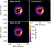 |
Fig. B.1. Multi-epoch detection of the spiral disk around HD 100453. The disk is imaged in K1 and reduced with RDI-DIsNMF to remove the direct starlight. The white star shows the position of the host star. |
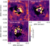 |
Fig. B.2. Residual images of disk-removed science data after the reduction of RDI-DIsNMF. No disk signal is left over, indicating a good recovery of disk flux. The white star shows the position of the host star. |
Appendix C: Determining the location of the spiral arm
To determine the local maxima of the spiral arm in polar coordinates, we performed two Gaussian profile fits with an additional constant, totaling seven free parameters. By doing so, we can simultaneously account for the existence of a ring-like structure near the IWA and that of a spiral. The additional constant was adopted in the model to account for the overall disk emission.
The regions with radii of < 14 pixels and > 35 pixels were masked out to avoid the noisy regions close to the IWA (8 pixels) and those without disk emissions, respectively. In each azimuthal angle (1° step) in the polar images we performed a fitting to obtain the location of the spiral arm and presented it in Figs. 2 and D.1. We visually inspected all fitting results to ensure the correctness of the fitting (i.e., that the data are reasonably represented by the model).
Appendix D: Uncertainty estimation
Precise motion measurements require accurate recovery of disk morphology. While RDI-DIsNMF can avoid the self-subtraction effect and it is theoretically expected to mitigate the overfitting of stellar PSFs, it may still slightly alter the disk morphology during PSF modeling since we cannot guarantee a perfect match of the speckles between a target image and its corresponding selected PSF references.
To account for this potential PSF mismatch effect, it is necessary to introduce additional uncertainty in spiral motion measurements. With the two K1 observations in 2019 obtained on different nights, the temporal separation is too small (1 day apart) to obtain spiral motion measurement. However, these two observations in 2019 are ideal in offering a unique opportunity to examine the unknown uncertainties in our dynamical analysis, especially in quantifying the change in disk morphology, and thus its impact on spiral motion caused by RDI-DIsNMF.
By measuring the motion of the spiral arms in two observations in 2019, we can estimate the motion caused by our post-processing method instead of the real spiral motion. Given the time span of ∼1 day, the real spiral motion is ∼0 degree. We performed the identical motion measurement procedure as in Sect. 3, and obtained a motion of  for the S1 arm in the two 2019 observations shown in Fig. D.1. Nevertheless, it is possible that the selected PSFs do not necessarily return such uncertainties for all the epochs studied here. Therefore, we conservatively consider an additional uncertainty of
  for the RDI-DIsNMF method.
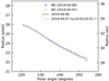 |
Fig. D.1. Peak locations of spiral arm S1 in polar coordinates after the correction for the viewing geometry. Solid curves represent the best-fit model spiral for the peak locations (dot) between two epoch observations in 2019, assuming the companion-driven scenario. Two curves (black and gray) are overlapped. The derived angular velocities of spiral pattern motion are |

In our analysis, the total uncertainty in our pattern speed analysis is
 (D.1)
(D.1)
where σfit, σnorth, and σRDI are uncertainties caused by the measurement of the spiral locations, true north uncertainty of SPHERE, and our post-processing method, respectively. The time span between two epochs is represented by t, which is 4.0 years.
The uncertainty of the spiral S1 locations returns a fitting uncertainty (σfit) of  . We adopt the true north uncertainty of SPHERE to be
  in all epochs (Maire et al. 2016). The uncertainty caused by the post-processing method is estimated to be
  per epoch using the 2019 observations. For the motion measurement on two epochs, σnorth is
  and σRDI is
  . Based on Equation (D.1), the final 1σ uncertainty on the pattern speed of the S1 arm is
  yr−1.
yr−1.
Appendix E: Effect of disk flaring on spiral motion measurement
Throughout the paper, we present the velocity of the spiral motion based on the best-fit model (h = 0.22 × r1.04) from Benisty et al. (2017) to correct for the disk flaring in the deprojection. The deprojection will affect the spiral location determination, and subsequently the spiral motion measurement. To study the effect of the disk flaring on spiral motion measurement, we adopted a reasonable range of parameters for correcting the disk flaring and performed new motion measurements, as described in Sect. 3.1. The effect of the disk flaring on spiral motion measurement is shown in Fig. E.1.
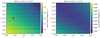 |
Fig. E.1. Effect of disk flaring on spiral motion measurement. Different disk flaring will change the spiral location determination in the deprojection, which affects the spiral motion measurement. Left panel: Spiral motions derived based on different disk flaring. Right panel: Corresponding uncertainties obtained using Equation D.1. The red dot represents the velocity of the spiral motion and its corresponding uncertainty based on the best-fit disk model (h = 0.22 × r1.04) from Benisty et al. (2017). |
In the case of HD 100453, the velocity of the spiral motion decreases with the increase in the disk flaring, ranging from  yr−1 to
  yr−1. This velocity range still favors the companion-driven scenario and disfavors the GI scenario. Given that different disk flarings only have a minor impact on the spiral motion and do not change our conclusion, we only present the motion measurement based on the best-fit model of disk flaring from Benisty et al. (2017).
Appendix F: Companion orbital fitting
We performed a linear fit to the position angles of HD 100453 B from 2003 to 2019. The astrometric data is listed in Table F.1, which was adopted from Collins et al. (2009), Wagner et al. (2018), and Gonzalez et al. (2020). The orbital period of the companion is about 800 years, which is significantly longer than the time span of our astrometric data. For the ∼20-year temporal separation studied here, the linear fit is therefore sufficient in obtaining the angular velocity of the companion. Figure F.1 shows the position angles of HD 100453 B and our linear fitting result. The slope corresponds to the measured angular velocity of the companion in the sky plane, which is  yr−1 in the counterclockwise direction. Using only two astrometry data sets in 2015 and 2019, we obtained an angular velocity of
  yr−1 in the sky plane, which validates the choice of a linear fit.
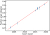 |
Fig. F.1. Linear fit to the position angles of HD 100453 B as the function of epochs. The slope corresponds to the measured angular velocity of the companion in the sky plane, which is |

Astrometric data
Appendix G: Companion orbital motion
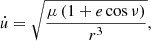
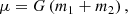
The companion orbit can be described by the orbital elements. The radial separation (r) between the companion and the primary star is
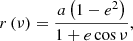 (G.1)
(G.1)
where ν, a, and e are the true anomaly, semimajor axis, and eccentricity, respectively.
We introduced u to represent the angle between the radial direction of the companion (r) and the intersection between the orbit and the sky planes. So the angle u is
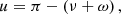 (G.2)
(G.2)
where ω is the argument of periastron.
The projected radial separation of the companion in the sky plane (rproj) is
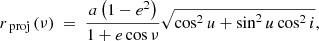 (G.3)
(G.3)
where i is the inclination between the orbital plane and the sky plane. Equation (G.3) shows the projection of the radial separation in Equation (G.1) onto the sky plane. For a given combination of orbital elements and the projected radial separation (rproj), we can obtain their corresponding true anomaly (ν) by solving Equation (G.3) numerically.
The specific angular momentum
 (G.4)
(G.4)
or
 (G.5)
(G.5)
where V is the velocity of the companion in the orbit and the symbol ⊥ donates the direction that is perpendicular to the outward radial from the primary to the companion. The orbit equation that defines the separation between the primary and the companion is
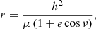 (G.6)
(G.6)
where h is the specific angular momentum. Substituting Equation (G.1) into Equation (G.6), we obtain
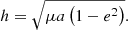 (G.7)
(G.7)
The definition of angular velocity is
 (G.8)
(G.8)
from which we can obtain the angular velocity of the companion at a given position in the orbital plane,
 (G.9)
(G.9)
where μ is the gravitational parameter. In our case, the gravitational parameter is a constant as
 (G.10)
where G, m1, and m2 are the gravitational constant, the mass of the primary (1.7 M⊙), and the mass of the companion (0.2 M⊙), respectively.
We use Vproj to represent the projection of V⊥ in the sky plane,
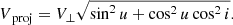 (G.11)
The velocity in the sky plane that is perpendicular to the projected radial separation (rproj) is
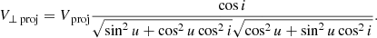 (G.12)
By substituting Equation (G.11) into Equation (G.12), we obtain
 (G.13)
The projected angular velocity of the companion in the sky plane is
 (G.14)
which can be rewritten as
 (G.15)
by substituting Equation (G.1), Equation (G.3), and Equation (G.13) into Equation (G.14). Equation (G.15) shows the projection of the angular velocity of the companion onto the sky plane.
We adopted the orbits of the companion from Gonzalez et al. (2020), which were derived from the astrometric fit to the companion positions listed in Table F.1. For a given combination of the orbital elements, we first use Equation (G.3) to numerically derive the true anomaly of the companion for a given orbit, adopting the separation rproj of 1.046″ in 2019. Based on Equation (G.1), Equation (G.2), Equation (G.9), and Equation (G.15), we can derive the angular velocity of the companion in the sky plane using only the orbital elements (i.e., a, e, ν, ω, i). Finally, we deprojected the angular velocity of the companion in the sky plane to the disk plane, adopting the disk inclination, the disk position angle, and the companion position angle as  ,
,  , and
, and  , respectively. The derived current angular velocity of the companion is
  yr−1. In Fig. 3, we present the calculated maximum velocity of the companion in the disk plane, which is
  yr−1. The uncertainties are (16th, 84th) percentiles in Bayesian statistics.
We also validated the posterior probability distribution of orbital parameters by using orbitize! (Blunt et al. 2017, 2020) and the same astrometric data shown in Table F.1. Based on the new orbital parameters, we obtained the current angular velocity and maximum velocity of the companion to be  yr−1 and
  yr−1, which is consistent with the results derived from Gonzalez et al. (2020).
Appendix H: Orbital parameters of the spiral-driving companion
In general, the spiral pattern motion should be in the range of the slowest and fastest companion orbital frequency in the scenario of an eccentric perturber (see Eq. 12 in Zhu & Zhang 2022). From the posterior probability distribution of orbital parameters obtained by Gonzalez et al. (2020), we derived the orbital parameters that satisfy Eq. 12 in Zhu & Zhang (2022). In this case, the maximum orbital velocity of the companion is greater than the minimum spiral motion ( yr−1). The corresponding distribution of orbital parameters is shown in Fig. H.1.
 |
Fig. H.1. Distribution of orbital parameters that can dynamically drive the spiral. |
All Tables
All Figures
|
Fig. 1. SPHERE/IRDIS detection of the HD 100453 system in K1, showing the companion and two spiral arms around a ring-like structure. The gray lines represent the companion orbits that can dynamically drive the spiral arm. The white star shows the position of the primary star. |
| In the text | |
|
Fig. 2. Peak locations of spiral arm S1 in polar coordinates after correction for viewing geometry. The solid curves represent the best-fit model spiral for the peak locations (dot points) between 2015 and 2019, assuming the companion-driven scenario. The derived angular velocities of spiral pattern motion are |
| In the text | |
|
Fig. 3. Angular velocity of the S1 spiral pattern motion in HD 100453 (black line). It could follow local Keplerian motion (green curve) or be smaller than the maximum value of the companion orbital motion (blue curve), under gravitational instability (GI) or companion–disk interaction, respectively. The measured spiral motion is consistent with the companion motion in the system and is inconsistent with the local Keplerian motion, revealing the companion-driven origin of the spiral arm S1, while excluding the GI origin. The motions here adopt a central stellar mass of 1.70 ± 0.09 M⊙. The colored shaded regions around each curve represent the corresponding uncertainties. |
| In the text | |
|
Fig. B.1. Multi-epoch detection of the spiral disk around HD 100453. The disk is imaged in K1 and reduced with RDI-DIsNMF to remove the direct starlight. The white star shows the position of the host star. |
| In the text | |
|
Fig. B.2. Residual images of disk-removed science data after the reduction of RDI-DIsNMF. No disk signal is left over, indicating a good recovery of disk flux. The white star shows the position of the host star. |
| In the text | |
|
Fig. D.1. Peak locations of spiral arm S1 in polar coordinates after the correction for the viewing geometry. Solid curves represent the best-fit model spiral for the peak locations (dot) between two epoch observations in 2019, assuming the companion-driven scenario. Two curves (black and gray) are overlapped. The derived angular velocities of spiral pattern motion are |
| In the text | |
|
Fig. E.1. Effect of disk flaring on spiral motion measurement. Different disk flaring will change the spiral location determination in the deprojection, which affects the spiral motion measurement. Left panel: Spiral motions derived based on different disk flaring. Right panel: Corresponding uncertainties obtained using Equation D.1. The red dot represents the velocity of the spiral motion and its corresponding uncertainty based on the best-fit disk model (h = 0.22 × r1.04) from Benisty et al. (2017). |
| In the text | |
|
Fig. F.1. Linear fit to the position angles of HD 100453 B as the function of epochs. The slope corresponds to the measured angular velocity of the companion in the sky plane, which is |
| In the text | |
|
Fig. H.1. Distribution of orbital parameters that can dynamically drive the spiral. |
| In the text | |
Current usage metrics show cumulative count of Article Views (full-text article views including HTML views, PDF and ePub downloads, according to the available data) and Abstracts Views on Vision4Press platform.
Data correspond to usage on the plateform after 2015. The current usage metrics is available 48-96 hours after online publication and is updated daily on week days.
Initial download of the metrics may take a while.