| Issue |
A&A
Volume 675, July 2023
|
|
|---|---|---|
| Article Number | A171 | |
| Number of page(s) | 11 | |
| Section | The Sun and the Heliosphere | |
| DOI | https://doi.org/10.1051/0004-6361/202345931 | |
| Published online | 14 July 2023 | |
The intensity ratio variation of the Si IV 1394/1403 Å lines during solar flares
Resonance scattering and opacity effects
1
School of Astronomy and Space Science, Nanjing University, 163 Xianlin Road, Nanjing 210023, PR China
e-mail: This email address is being protected from spambots. You need JavaScript enabled to view it.
2
Key Laboratory for Modern Astronomy and Astrophysics (Nanjing University), Ministry of Education, 163 Xianlin Road, Nanjing 210023, PR China
Received:
18
January
2023
Accepted:
7
June
2023
Abstract
Context. The Si IV lines at 1394 Å and 1403 Å form in the solar atmosphere at a temperature of ∼104.8 K. They are usually considered optically thin, but their opacity can be enhanced during solar flares. Traditionally, the intensity ratio of these lines are used as an indicator of the optical thickness. However, observations have shown a wavelength-dependent intensity ratio profile r(Δλ) of the 1394 Å to 1403 Å lines.
Aims. We aim to study the variation of the intensity ratio profile in solar flares and the physical reasons behind it.
Methods. The Si IV lines and their intensity ratio profiles were calculated from the one-dimensional radiative hydrodynamics flare model with nonthermal electron heating.
Results. During flares, r(Δλ) is smaller than two at the line core but larger than two at the line wings. We attribute the deviation of the ratio from two to the following two effects: the resonance scattering effect and the opacity effect. Resonance scattering increases the population ratio of the upper levels of the two lines, and, as a result, increases r(Δλ) in all wavelengths. The opacity effect decreases r(Δλ), especially at the line core where the opacity is larger. These two effects compete with each other and cause the U shape of r(Δλ).
Key words: Sun: chromosphere / line: profiles / radiative transfer / opacity
© The Authors 2023
 Open Access article, published by EDP Sciences, under the terms of the Creative Commons Attribution License (https://creativecommons.org/licenses/by/4.0), which permits unrestricted use, distribution, and reproduction in any medium, provided the original work is properly cited.
This article is published in open access under the Subscribe to Open model. This email address is being protected from spambots. You need JavaScript enabled to view it. to support open access publication.
1. Introduction
The transition region (TR) is a thin layer between the chromosphere and the corona, where the physical quantities change dramatically in the Sun. The temperature could change by several orders of magnitude, and a number of emission lines form in the TR, such as the Si IV, C IV, O IV, and Ne VII lines, which could reveal the dynamic properties of local plasma. The Si IV resonance lines at 1394 Å and 1403 Å are two typical TR lines with a formation temperature of ∼104.8 K. It is generally accepted that photons generated in the TR are able to escape from the solar surface without absorption or scattering; that is, these lines are usually considered optically thin. Under the optically thin assumption, Mathioudakis et al. (1999) indicated that, for pairs of resonance lines such as Si IV 1394/1403 Å and C IV 1548/1551 Å that share the same lower level but different upper levels, the ratio of the line intensities is exactly the ratio of the oscillator strengths of the two lines. This ratio is 0.52:0.26 = 2:1 for the Si IV 1394/1403 Å lines (Maniak et al. 1993). Usually, a decrease from two implies that there is an opacity effect along the line of sight.
During heating events such as transient brightenings in the TR or solar flares, the atmosphere is heated to a high temperature where the Si IV lines could be significantly enhanced. Recent works suggest that the optically thin assumption of the Si IV lines does not hold in some cases. Yan et al. (2015) found the self-absorption effect on both Si IV lines for the first time. They found that the intensity ratio is reduced to 1.7 ∼ 2. The same effect has also been reported in Nelson et al. (2017). Tripathi et al. (2020) studied the distribution of intensity ratios in active regions. They conclude that there are a considerable number of pixels where the intensity ratio deviates from two, especially in the early phases of flares and in parts of flare ribbons. Recent radiative hydrodynamic simulations indicate that the two Si IV lines might not be optically thin in flare conditions (Kerr et al. 2019), where the intensity ratio varies from 1.8 to 2.3.
It should be pointed out that the intensity ratio could also be larger than two in many observations (Tripathi et al. 2020; Zhou et al. 2022), where the opacity effect fails to explain this. Previous studies attributed this to the result of resonance scattering, which implies that a stronger resonance scattering yields a larger intensity ratio (Gontikakis & Vial 2018; Gontikakis et al. 2013).
The abovementioned intensity ratio usually refers to the ratio of wavelength-integrated intensity R = ∫I1394 Å(λ)dλ/∫I1403 Å(λ)dλ as adopted in previous studies. However, considering that the opacity at the line core is much larger than that at the line wings, the intensity ratio may also vary from the line core to the line wings. Zhou et al. (2022) focused on the wavelength-dependent intensity ratio profile r(Δλ) = I1394 Å(Δλ)/I1403 Å(Δλ). They found that at the flare ribbons, r(Δλ) is less than two at the line core and larger than two at the line wings, while the ratio of the integrated intensity is still close to two. It is suggested that the intensity ratio profile r(Δλ) serves as a better proxy for the line opacity. Thus, the variation of r(Δλ) along the wavelength deserves further investigation.
In this paper, we study the intensity ratio profile r(Δλ) of the Si IV resonance lines in one-dimensional radiative hydrodynamic flare models. We examine the variation of the intensity ratio along the wavelength and explore possible physical mechanisms. The flare models and calculation of the Si IV lines are briefly described in Sect. 2. The spectral line profiles and intensity ratio profiles r(Δλ) are shown in Sect. 3. Reasons for the variation of r(Δλ) are discussed in Sect. 4. Finally we make conclusions in Sect. 5.
2. Method
The one-dimensional radiative hydrodynamics code "RADYN" was first used to study shocks in the chromosphere (Carlsson & Stein 1992, 1997, 1995), but now it is more often employed for the response of the solar atmosphere during flares (Allred et al. 2015). The conservation equations of mass, momentum, energy, and charge coupled with atom level population equations and radiative transfer equations are solved in a one-dimensional plane-parallel atmosphere, on an adaptive grid (Dorfi & Drury 1987). The initial atmosphere is based on the VAL3C model, with a 10 Mm semicircular flare loop. The loop-top temperature is 10 MK. To simulate the heating by flares, a high-energy nonthermal electron beam was injected from the loop top, and then moved downward along the flare loop. A set of three parameters describes the power-law energy distribution of nonthermal electrons: the cutoff energy Ec, the spectral index δ, and the energy flux F. The former two parameters were fixed in each simulation run, while the energy flux rose with time linearly to a peak Fpeak at 10 s, and then fell linearly to zero at 20 s. We have made a grid of 25 simulations by varying Ec from 5 to 25 keV and varying δ from three to seven, where Fpeak is fixed at 1010 erg s−1 cm−2. We find that a large value of Ec causes stronger heating at large column depth and a small value of δ makes the heating more concentrated. The variation of Ec and δ causes different heating rates with height and different intensities of profiles, while the distribution of line ratios and population ratios do not change qualitatively. Thus, we only show three typical cases here. In addition, we also show another simulation with a larger Fpeak (1011 erg s−1 cm−2) where the line profiles show central reversals. These four cases are described in Table 1, where the notations are the same as in Hong et al. (2022), and the other 22 cases are listed in Appendix A. The heating rate of the flaring atmosphere was calculated with the Fokker-Plank approach. We ran each simulation for 20 s.
Parameters of flare models.
The minority species version of the code ("MSRADYN") was employed to calculate the Si IV lines which do not significantly contribute to the atmosphere. We followed the atmosphere of the main run, and solved the level populations and radiative transfer equations for the silicon atom only (Kerr et al. 2019). The Si model atom is the same as in Kerr et al. (2019). The snapshot of the simulations were saved every 0.1 s.
3. Result
3.1. The intensity ratio profile r(Δλ)
The time evolution of the Si IV intensity profiles and the intensity ratio profile r(Δλ) for the four simulation cases are shown in Fig. 1. At each wavelength, we subtracted the averaged intensity value at far wings (±1 Å) from the profile to eliminate the influence of the continuum. Such a subtraction was carried out for every timestep. From the intensity profiles, one can see clearly that the Si IV intensity is enhanced after a certain time of heating, when sufficient energy is deposited in the upper chromosphere (1.4 − 1.8 Mm) and the number of Si IV atoms is increased. For the first three cases, the line profiles show a single peak that is gradually blueshifted, indicating the upflow of chromospheric evaporation (Li et al. 2019; Kerr et al. 2019). Comparing the first three panels, we can find some differences in the profiles when changing the spectral index δ and the cutoff energy Ec. A larger value of δ and a smaller value of Ec means that the electrons are mostly distributed in the lower-energy part, which cause faster and stronger heating at a low column depth, corresponding to the earlier enhancement and greater intensity, respectively. We note that for Case f10E25d7, the top part of the chromosphere is undisturbed and becomes trapped between the heated chromosphere and the TR, forming a “chromospheric bubble” (Reid et al. 2020). For Case f11E25d3 (Fig. 2), the line profiles show multipeaks from t = 5 s and last for the whole flare. The central reversal caused by absorption in the line core suggests a large opacity at −0.5 Å, and an additional red component at around 0.8 Å serves as a result of condensation downflows (Tian et al. 2022).
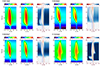 |
Fig. 1. Time evolution of the Si IV line profiles (1394 Å on the left) and the intensity ratio profiles r(Δλ) in all four flare models. Black, red, and blue lines show wavelength positions that were specifically chosen to represent the line core (Δλc), the red wing (Δλr), and the blue wing (Δλb) at each time, respectively, which are defined in Sect. 3.1. |
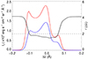 |
Fig. 2. Line profiles of Si IV 1394 Å (red line), Si IV 1403 Å (blue line), and the intensity ratio profile r(Δλ), (black line) at t = 10 s for Case f11E25d3. |
The intensity ratio profile stays close to two before the obvious enhancement of the Si IV line profiles. A variation of the ratio at different wavelengths is clearly shown, where the ratio at the line wings is generally larger than two, while the ratio at the line core is generally smaller than two. For each intensity ratio profile, we chose three specific wavelength positions to represent the line core (Δλc), the blue wing (Δλb), and the red wing (Δλr), respectively, which are overplotted in Fig. 1. The centroid of the Si IV 1403 Å intensity profile was chosen as Δλc. The values of Δλb and Δλr were specifically chosen so that  , where the integration range [Δλmin, Δλmax] is [−0.5 Å, 0.5 Å]. In Fig. 3 we show the ratio of wavelength-integrated intensity R and the wavelength-dependent ratio r(Δλ) at these wavelength positions. It is obvious that after a certain time of heating, r(Δλb) and r(Δλr) are generally larger than R, and r(Δλc) tends to be smaller than R. The value of r(Δλ) can reach as high as 3.5 at the line wings and as low as 1.5 at the line center, while the value of R is still close to two owing to an integration effect. The variation behavior of r(Δλ) and the quantity of R are quite similar to observations at flare ribbons (Zhou et al. 2022).
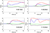 |
Fig. 3. Time variations of the ratio at the red wing (red solid line), the blue wing (blue solid line), the line core (black solid line), and the ratio of integrated intensity (green solid line) in four cases. The wavelength positions for the line core, the red wing, and the blue wing in each case are marked in Fig. 1. |
3.2. The optical thickness
Previous studies have suggested that the opacity cannot be neglected when we calculate the Si IV resonance lines during strong flares (Kerr et al. 2019). To understand the opacity effect in line formation, calculating the contribution function is useful (Caccin et al. 1977; Magain 1986). The analytic solution of the radiative transfer equation is
 (1)
(1)
where μ = cosθ and θ is the angle between the observer and the vertical direction. We used μ ≈ 1 for this work. Furthermore, Sλ(τλ) and τλ are the source function and the optical depth, respectively. We used the variable dz (geometrical depth) instead of dτλ to get another form:
 (2)
(2)
where jλ(z) is the emissivity and Cλ is the contribution function with respect to wavelength per height. We can get the emergent intensity by integrating the contribution function along the light path.
Hereby we employ Case f10E25d3 as an example. The results from three other cases do not show qualitative differences, and are together shown in Appendix B. Figure 4 shows the contribution function of the Si IV 1403 Å line. At each wavelength, the contribution function mainly peaks at two heights, and this is contributed to by continuum emission from the temperature minimum region and line emission in the upper chromosphere and the TR, respectively. At t = 0 s, the contribution function at the Si IV 1403 Å line center gathers at z ≈ 1.8 Mm, indicating that the line is mainly formed in the TR.
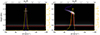 |
Fig. 4. Line formation of the Si IV 1403 Å line in Case f10E25d3, for t = 0 s on the left panel and t = 10 s on the right panel. Background gray shades represent the contribution function. Blue lines denote the vertical velocity and red lines denote the τλ = 1 height. Orange lines refer to the line profiles. |
The height where τλ = 1 is at around 0.5 Mm at this moment, where the continuum is formed, which is far lower than the TR. The opacity at the line formation region is quite small where the absorption can be neglected safely, and thus the line can be regarded as optically thin. At t = 10 s, the region between 1.5 Mm and 2 Mm that is heated intensively now mostly contributes to the line emission. Meanwhile, the τλ = 1 curve also rises to z ≈ 1.6 Mm around the line core, which implies that the opacity in the line formation region is now nonnegligible (Kerr et al. 2019).
We show the intensity ratio profile r(Δλ) and the optical depth at the line formation height τh as functions of wavelength in Fig. 5. The formation height is defined as the centroid of the contribution function (Leenaarts et al. 2012).
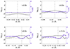 |
Fig. 5. Optical depth at the line formation height τh (black line) and the intensity ratio profile r(Δλ), (blue solid line) for Case f10E25d3. We only show the wavelength range at which the emergent intensity is larger than three times the continuum. The blue dashed lines show r(Δλ) which is degraded to the IRIS spectral resolution (0.026 Å). Overplotted are the horizontal line of r = 2 and the vertical line for the position of the line core. |
At t = 0 s, τh at the line core is smaller than 0.01, which means the opacity effect here is not important, and it is reasonable to treat these lines as optically thin. When the atmosphere is heated during solar flares, τh also increases dramatically, especially at the line core. At t = 10 s, τh is larger than one at the line core, corresponding to the rise of the τλ = 1 curve around the line core in Fig. 1. One needs to consider the optical effect at this time, although it is still optically thin at the far wings.
The variation of r(Δλ) seems to be negatively correlated to the variation of τh. The intensity ratio r(Δλ) decreases from the line wings to the line core, while the optical depth τh increases. In each intensity ratio profile, the normalized ratio rn(Δλ) is defined as follows: rn(Δλ) = r(Δλ)/rmax. In Fig. 6 we show a scatter plot of the optical depth τh and the normalized ratio rn at each wavelength point at different times from all four simulation cases. A negative tendency is clearly shown in the figure, which implies that the opacity has an obvious effect on decreasing the intensity ratio. We discuss the reason for this in Sect. 4.2.
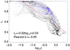 |
Fig. 6. Scatter plot of the normalized ratio (rn) versus the optical depth at the formation height (τh) for four cases. Blue dots come from Case f10E25d3. The red line shows the result of a linear fit of all the data points. |
3.3. The population ratio of the Si IV 3p levels
The two resonance lines of Si IV share the same lower-energy level 3s, but they have different higher levels at 3p. We hereby label the energy levels at 3s (2S1/2) and 3p (2P1/2 and 2P3/2) as levels 0, 1, and 2, respectively, in the order of increasing energies. Thus, the population densities at the three levels are denoted as n0, n1, and n2, respectively. The two 3p levels are so close that n2/n1 is considered to be the ratio of their statistical weights in Local Thermodynamic Equilibrium (LTE) assumption (Rathore & Carlsson 2015).
We show the population ratio n2/n1 in dependence of height and time in Fig. 7, together with the contribution function at the line core. At t = 0 s, the population ratio stays close to two in the line formation region (around 1.8 − 1.9 Mm). We notice that in the chromosphere the population ratio is much larger than two where there is very little contribution to the line intensity. We discuss why n2/n1 > 2 in Sect. 4.1.
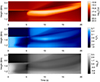 |
Fig. 7. Time evolution of the height distribution of the contribution function at the line core (top panel), the population ratio n2/n1 (middle panel), and the proportion of the resonance scattering to thermal emission X (bottom panel) for Case f10E15d3. An obvious enhancement of the contribution function in the chromosphere starts from t = 5.0 s. |
As shown in Fig. 1, at around t = 5 s, the chromosphere is heated to ∼104 K and the Si IV line is being enhanced. The contribution function begins to show another peak at around 1.6 Mm from t = 5.0 s, and the population ratio above 1.8 Mm starts to increase in the meantime. After t = 6.0 s, the contribution function is dominant in the chromosphere, and the population ratio n2/n1 is larger than two in the layers where the line forms. Checking the results of all four simulation cases, we find an interesting fact that the second Cλ peak and the deviation of n2/n1 from two are closely related both spatially and temporally, which also correspond to the enhancement of Si IV lines.
4. Discussion
4.1. The deviation of the population ratio from two
The upper levels of the Si IV 1394 Å and Si IV 1403 Å lines are the fine structures of Si IV 3p electron configuration when the degeneracy of the orbital quantum number is broken. The statistical weight is four for the 3p 2P3/2 level (the upper level for the Si IV 1394 Å transition), and two for the 3p 2P1/2 level (the upper level for the Si IV 1403 Å transition). Under the LTE assumption, the population ratio n2/n1 is described by the Boltzmann equation,
 (3)
(3)
where g1 and g2 are statistical weights of level 1 and level 2, respectively. The energy level difference Δϵ is so small that  . Hence, the population ratio n2/n1 is considered to be equal to g2/g1, which is two exactly. However, the LTE assumption is no longer valid above the photosphere. At the chromosphere and the TR, the non-LTE effect is dominant.
We write the population equations for levels 1 and 2 (the 3p levels) as follows:
 (4)
(4)
 (5)
(5)
where Rij and Cij denote the radiative and collisional transition rates, and the subscript c represents the continuum level of Si IV.
In Fig. 8 we compare all the transition rates in Eq. (4) at 6.0 s, where  . It is very clear that in the line formation region, the transition rates between level 0 and level 1 are orders of magnitude larger than the rates of other transitions. The dominant terms are collisional and radiative excitations plus spontaneous emission. Considering that the time derivatives of the level populations are very small (see Fig. 8), we further simplified Eqs. (4) and (5) by including only the dominant terms:
 (6)
(6)
 (7)
(7)
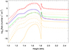 |
Fig. 8. Height distribution of all the transition rates in Eq. (4) for Case f10E25d3 at 6.0 s. Red lines represent the transitions between levels 0 and 1: n0C01 (red solid line), n1C10 (red dotted line), n0R01 (red dashed line), n1A10 (red dotted-dashed line), and |

The transitions can be divided into two processes: collisional excitation followed by radiative deexcitation, which corresponds to thermal emission; and radiative excitation followed by radiative deexcitation, which is referred to as resonance scattering (Gontikakis & Vial 2018). Assuming that  and noticing that A20/A10 = 1, C02/C01 = B02/B01 = 2, we obtained
 (8)
(8)
where  is the proportion of the resonance scattering to thermal emission. We can find that the population ratio is positively correlated with the value of X, that is, the increase in resonance scattering makes n2/n1 > 2.
The above mechanism is illustrated in the bottom panel of Fig. 7. At t = 0 s, the radiation is small enough (X ≪ 1) in the line formation region (1.8 − 1.9 Mm), and the population ratio is two according to Eq. (8), which is also the result under coronal approximation. After a certain time of flare heating (5 s in Case f10E25d3), the local radiation is enhanced and the radiative excitation rate is comparable to the collisional excitation rate. The population ratio also increases gradually with time and becomes larger than two in the line formation region (Fig. 7).
4.2. The deviation of the intensity ratio from two
We now discuss how the population ratio would influence the line intensity ratio. We first considered the optically thin case where the optical depth is so small that e−τλ ≈ 1, and Cλ ≈ jλ. Thus we could obtain the emergent intensity by only integrating the emissivity along the height:
 (9)
(9)
 (10)
(10)
where ψ(z, Δλ) are normalized profiles. Noticing that A20 = A10, ψ1394 Å(z,Δλ) ≈ ψ1403 Å(z,Δλ), the ratio of emergent intensity only depends on the population ratio n2/n1. At t = 0 s, the Si IV lines are optically thin, and the intensity ratio stays close to two (Fig. 5), which is equal to the population ratio n2/n1 (Fig. 7).
In flare conditions, we need to consider the optical depth term in the contribution function. The intensity ratio is related to the ratio of the contribution functions since the integration range is the same. The ratio of contribution functions is given as
 (11)
(11)
which is a function of wavelength and height. As we has shown above, a deviation of the ratio n2/n1 from two is mainly from the resonance scattering effect, while the term  apparently represents the opacity effect. At each height, the ratio of the contribution function is reduced by the opacity effect because τ1394 Å > τ1403 Å. As a result, the intensity ratio is reduced by the opacity effect. However, when the population ratio n2/n1 grows due to resonance scattering, the intensity ratio increases proportionally. These two effects compete with each other. Besides their opposite effects on the magnitude of the intensity ratio, the effect of n2/n1 is wavelength independent while that of τ is wavelength dependent.
The intensity ratio profiles in Fig. 1 could then be explained as follows. The resonance scattering effect elevates the intensity ratio r(Δλ) to larger than two, while the opacity effect pulls the ratio back to some extent. At the line center, the opacity is relatively larger so that the intensity ratio is pulled back by a larger amount, causing a U-shaped profile. The ratio at the line wings are generally larger than two, while the ratio at the line core could be larger or smaller than two, depending on how much effect the opacity exerts on the ratio.
We further illustrate these two effects by defining the difference of the contribution functions as ΔC(Δλ,z) = C1394 Å(Δλ,z) − 2C1403 Å(Δλ,z). The integration of ΔC in height gives the difference of intensities I1394 Å(Δλ) − 2I1403 Å(Δλ). Therefore, the value of ΔC indicates the contribution to the deviation of r(Δλ) from two. A positive ΔC tends to elevate r(Δλ) to over two, while a negative one tends to suppress r(Δλ) to below two.
In Fig. 9 we show the distribution of ΔC at t = 8.0 s for Case f10E25d3. We note that ΔC is normalized at each wavelength. At each wavelength, the region where ΔC > 0 is located in the upper chromosphere (1.6–1.9 Mm). It is also the line formation region where the contribution function Cλ is large and resonance scattering is strong (X > 1). However, the region where ΔC < 0 only appears in the line core, coinciding with the region with a large opacity.
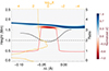 |
Fig. 9. Normalized difference of the contribution functions (ΔC) at 8.0 s in Case f10E25d3 (background). The intensity ratio profile is marked as the black line. The red line denotes the τ = 1 height and the orange line refers to the proportion of resonance scattering to thermal emission (X). |
Thus, the r(Δλ) profile shows a U shape, in which the ratio increases toward the line wings but decreases toward the line core. Similar features of r(Δλ) and ΔC are found in other simulation cases during flare heating.
4.3. Comparison with observations
In Fig. 5, we also plotted the ratio of the intensity profiles that are degraded to the spectral resolution of Interface Region Imaging Spectrograph (0.026 Å). One can see that the U-shaped profile is still obvious, with the value at the line core being smaller than two, while the value at the line wings is larger than two. In fact, such U-shaped profiles have been reported in previous observations (Zhou et al. 2022).
The central reversal in emission lines is often caused by the large line opacity. In observations there are reports of such features in the Si IV lines, especially in flares (Yan et al. 2015; Zhou et al. 2022; Lörinčík et al. 2022). In our simulations, we find centrally reversed profiles in Case f11E25d3 (Fig. 2), where the energy flux F is one order of magnitude higher than that in three other cases. We confirm that the central reversal is due to the increased line opacity.
In many observations of the Sun or other stars, the ratio of integrated intensity R is taken as an indicator of the optical thickness (Mathioudakis et al. 1999; Christian et al. 2006; Yan et al. 2015; Brannon et al. 2015; Mulay & Fletcher 2021). Zhou et al. (2022) claim that the wavelength-dependent ratio profile r(Δλ) would be a better indicator since the opacities at the line core and at the line wings are different. Our results confirm that the intensity ratio profile r(Δλ) usually has a U shape as in observations. However, we find it still insufficient in some cases to use the value of either R or r(Δλ) as an indicator of the optical thickness. For example, in the simulation snapshot of Case f10E25d3 at 6.0 s, both R and the intensity ratio at the line core r(Δλc) are larger than two, but we do see an obvious increase in the line opacity (Fig. 5). The normalized ratio rn might be a complementary indicator of the optical thickness as judged from Fig. 6. Quantitatively, the Si IV line is not optically thin anymore if rn < 0.6.
5. Conclusions
In this paper, we analyze the properties of the two Si IV resonance lines in flare conditions based on "RADYN" simulations. We focus on the intensity ratio profile r(Δλ) and find that the value of r(Δλ) rises at the line wings and falls at the line core. By comparison, the ratio of integrated intensity R lies between the minimum and maximum of r(Δλ). At most of the wavelength points, r(Δλ) deviates from two obviously, ranging from 1.5 to four. However, R usually ranges from 1.8 to 2.3. We agree with Kerr et al. (2019) that the opacity of the two resonance lines are both nonnegligible when a flare occurs. In the line core, the line opacity is larger and r(Δλ) becomes smaller than that in the line wings. By calculating the normalized ratio rn(Δλ) = r(Δλ)/rmax, we can quantitatively estimate the optical depth at the line formation height through an empirical relationship between rn and τ (Fig. 6).
We also find that due to flare heating, the increased rate of resonance scattering increases the population ratio of the Si IV 3p levels (n2/n1), which in turn increases the intensity ratio r(Δλ). In the mean time, the large opacity at the line core tends to decrease the intensity ratio r(Δλ). The competition of the resonance scattering effect and the opacity effect results in a U-shaped intensity ratio profile as in observations.
As noted above, the values of R and r(Δλ) are influenced by both resonance scattering and opacity. In the case that R and r(Δλ) are not sufficient to judge the optical thickness, we propose to use the normalized ratio rn(Δλ) as a complementary criterion. We conclude that if rn < 0.6, the line should be regarded as optically thick. Such a case most likely appears at the line core. On the other hand, since the opacity at the far wings is always small, a deviation from the intensity ratio r(Δλ) of two can safely serve as an indicator of the strength of resonance scattering.
Acknowledgments
We are grateful to the referee for careful reading of the paper and constructive comments. We would like to thank Graham Kerr for providing the Si IV model atom. This work was supported by National Key R&D Program of China under grant 2021YFA1600504 and by NSFC under grants 11903020 and 12127901.
References
- Allred, J. C., Kowalski, A. F., & Carlsson, M. 2015, ApJ, 809, 104 [NASA ADS] [CrossRef] [Google Scholar]
- Brannon, S. R., Longcope, D. W., & Qiu, J. 2015, ApJ, 810, 4 [NASA ADS] [CrossRef] [Google Scholar]
- Caccin, B., Gomez, M. T., Marmolino, C., & Severino, G. 1977, A&A, 54, 227 [NASA ADS] [Google Scholar]
- Carlsson, M., & Stein, R. F. 1992, ApJ, 397, L59 [Google Scholar]
- Carlsson, M., & Stein, R. F. 1995, ApJ, 440, L29 [Google Scholar]
- Carlsson, M., & Stein, R. F. 1997, ApJ, 481, 500 [Google Scholar]
- Christian, D. J., Mathioudakis, M., Bloomfield, D. S., et al. 2006, A&A, 454, 889 [NASA ADS] [CrossRef] [EDP Sciences] [Google Scholar]
- Dorfi, E. A., & Drury, L. O. 1987, J. Comput. Phys., 69, 175 [NASA ADS] [CrossRef] [Google Scholar]
- Gontikakis, C., & Vial, J. C. 2018, A&A, 619, A64 [NASA ADS] [CrossRef] [EDP Sciences] [Google Scholar]
- Gontikakis, C., Winebarger, A. R., & Patsourakos, S. 2013, A&A, 550, A16 [NASA ADS] [CrossRef] [EDP Sciences] [Google Scholar]
- Hong, J., Carlsson, M., & Ding, M. D. 2022, A&A, 661, A77 [NASA ADS] [CrossRef] [EDP Sciences] [Google Scholar]
- Kerr, G. S., Carlsson, M., Allred, J. C., Young, P. R., & Daw, A. N. 2019, ApJ, 871, 23 [NASA ADS] [CrossRef] [Google Scholar]
- Leenaarts, J., Carlsson, M., & Rouppe van der Voort, L. 2012, ApJ, 749, 136 [NASA ADS] [CrossRef] [Google Scholar]
- Li, Y., Ding, M. D., Hong, J., Li, H., & Gan, W. Q. 2019, ApJ, 879, 30 [NASA ADS] [CrossRef] [Google Scholar]
- Lörinčík, J., Polito, V., De Pontieu, B., Yu, S., & Freij, N. 2022, Front. Astron. Space Sci., 9, 1040945 [CrossRef] [Google Scholar]
- Magain, P. 1986, A&A, 163, 135 [NASA ADS] [Google Scholar]
- Maniak, S. T., Träbert, E., & Curtis, L. J. 1993, Phys. Lett. A, 173, 407 [CrossRef] [Google Scholar]
- Mathioudakis, M., McKenny, J., Keenan, F. P., Williams, D. R., & Phillips, K. J. H. 1999, A&A, 351, L23 [NASA ADS] [Google Scholar]
- Mulay, S. M., & Fletcher, L. 2021, MNRAS, 504, 2842 [NASA ADS] [CrossRef] [Google Scholar]
- Nelson, C. J., Freij, N., Reid, A., et al. 2017, ApJ, 845, 16 [Google Scholar]
- Rathore, B., & Carlsson, M. 2015, ApJ, 811, 80 [NASA ADS] [CrossRef] [Google Scholar]
- Reid, A., Zhigulin, B., Carlsson, M., & Mathioudakis, M. 2020, ApJ, 894, L21 [NASA ADS] [CrossRef] [Google Scholar]
- Tian, J., Hong, J., Li, Y., & Ding, M. D. 2022, A&A, 668, A96 [NASA ADS] [CrossRef] [EDP Sciences] [Google Scholar]
- Tripathi, D., Nived, V. N., Isobe, H., & Doyle, G. G. 2020, ApJ, 894, 128 [CrossRef] [Google Scholar]
- Yan, L., Peter, H., He, J., et al. 2015, ApJ, 811, 48 [NASA ADS] [CrossRef] [Google Scholar]
- Zhou, Y.-A., Hong, J., Li, Y., & Ding, M. D. 2022, ApJ, 926, 223 [NASA ADS] [CrossRef] [Google Scholar]
Appendix A: Additional simulation cases
Additional 22 simulation cases.
Appendix B: Additional figures
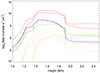 |
Fig. B.10. Same as Figure 8, but for Case f10E15d3. |
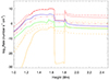 |
Fig. B.11. Same as Figure 8, but for Case f10E25d7. |
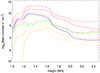 |
Fig. B.12. Same as Figure 8, but for Case f11E25d3. |
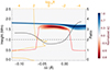 |
Fig. B.13. Same as Figure 9, but for Case f10E15d3. |
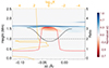 |
Fig. B.14. Same as Figure 9, but for Case f10E25d7. |
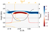 |
Fig. B.15. Same as Figure 9, but for Case f11E25d3. |
All Tables
All Figures
|
Fig. 1. Time evolution of the Si IV line profiles (1394 Å on the left) and the intensity ratio profiles r(Δλ) in all four flare models. Black, red, and blue lines show wavelength positions that were specifically chosen to represent the line core (Δλc), the red wing (Δλr), and the blue wing (Δλb) at each time, respectively, which are defined in Sect. 3.1. |
| In the text | |
|
Fig. 2. Line profiles of Si IV 1394 Å (red line), Si IV 1403 Å (blue line), and the intensity ratio profile r(Δλ), (black line) at t = 10 s for Case f11E25d3. |
| In the text | |
|
Fig. 3. Time variations of the ratio at the red wing (red solid line), the blue wing (blue solid line), the line core (black solid line), and the ratio of integrated intensity (green solid line) in four cases. The wavelength positions for the line core, the red wing, and the blue wing in each case are marked in Fig. 1. |
| In the text | |
|
Fig. 4. Line formation of the Si IV 1403 Å line in Case f10E25d3, for t = 0 s on the left panel and t = 10 s on the right panel. Background gray shades represent the contribution function. Blue lines denote the vertical velocity and red lines denote the τλ = 1 height. Orange lines refer to the line profiles. |
| In the text | |
|
Fig. 5. Optical depth at the line formation height τh (black line) and the intensity ratio profile r(Δλ), (blue solid line) for Case f10E25d3. We only show the wavelength range at which the emergent intensity is larger than three times the continuum. The blue dashed lines show r(Δλ) which is degraded to the IRIS spectral resolution (0.026 Å). Overplotted are the horizontal line of r = 2 and the vertical line for the position of the line core. |
| In the text | |
|
Fig. 6. Scatter plot of the normalized ratio (rn) versus the optical depth at the formation height (τh) for four cases. Blue dots come from Case f10E25d3. The red line shows the result of a linear fit of all the data points. |
| In the text | |
|
Fig. 7. Time evolution of the height distribution of the contribution function at the line core (top panel), the population ratio n2/n1 (middle panel), and the proportion of the resonance scattering to thermal emission X (bottom panel) for Case f10E15d3. An obvious enhancement of the contribution function in the chromosphere starts from t = 5.0 s. |
| In the text | |
|
Fig. 8. Height distribution of all the transition rates in Eq. (4) for Case f10E25d3 at 6.0 s. Red lines represent the transitions between levels 0 and 1: n0C01 (red solid line), n1C10 (red dotted line), n0R01 (red dashed line), n1A10 (red dotted-dashed line), and |
| In the text | |
|
Fig. 9. Normalized difference of the contribution functions (ΔC) at 8.0 s in Case f10E25d3 (background). The intensity ratio profile is marked as the black line. The red line denotes the τ = 1 height and the orange line refers to the proportion of resonance scattering to thermal emission (X). |
| In the text | |
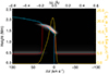 |
Fig. B.1. Same as Figure 4, but for Case f10E15d3 at t = 10 s. |
| In the text | |
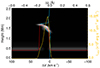 |
Fig. B.2. Same as Figure 4, but for Case f10E25d7 at t = 10 s. |
| In the text | |
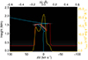 |
Fig. B.3. Same as Figure 4, but for Case f11E25d3 at t = 10 s. |
| In the text | |
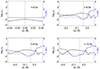 |
Fig. B.4. Same as Figure 5, but for Case f10E15d3. |
| In the text | |
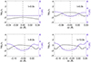 |
Fig. B.5. Same as Figure 5, but for Case f10E25d7. |
| In the text | |
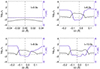 |
Fig. B.6. Same as Figure 5, but for Case f11E25d3. |
| In the text | |
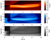 |
Fig. B.7. Same as Figure 7, but for Case f10E15d3. |
| In the text | |
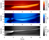 |
Fig. B.8. Same as Figure 7, but for Case f10E25d7. |
| In the text | |
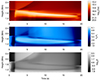 |
Fig. B.9. Same as Figure 7, but for Case f11E25d3. |
| In the text | |
|
Fig. B.10. Same as Figure 8, but for Case f10E15d3. |
| In the text | |
|
Fig. B.11. Same as Figure 8, but for Case f10E25d7. |
| In the text | |
|
Fig. B.12. Same as Figure 8, but for Case f11E25d3. |
| In the text | |
|
Fig. B.13. Same as Figure 9, but for Case f10E15d3. |
| In the text | |
|
Fig. B.14. Same as Figure 9, but for Case f10E25d7. |
| In the text | |
|
Fig. B.15. Same as Figure 9, but for Case f11E25d3. |
| In the text | |
Current usage metrics show cumulative count of Article Views (full-text article views including HTML views, PDF and ePub downloads, according to the available data) and Abstracts Views on Vision4Press platform.
Data correspond to usage on the plateform after 2015. The current usage metrics is available 48-96 hours after online publication and is updated daily on week days.
Initial download of the metrics may take a while.