| Issue |
A&A
Volume 675, July 2023
Solar Orbiter First Results (Nominal Mission Phase)
|
|
|---|---|---|
| Article Number | A20 | |
| Number of page(s) | 10 | |
| Section | The Sun and the Heliosphere | |
| DOI | https://doi.org/10.1051/0004-6361/202245747 | |
| Published online | 29 June 2023 | |
The source of unusual coronal upflows with photospheric abundance in a solar active region⋆
1
PMOD/WRC, Dorfstrasse 33, 7260 Davos, Switzerland
e-mail: louise.harra@pmodwrc.ch
2
ETH Zürich, Institute for Particle Physics and Astrophysics, Wolfgang-Pauli-Strasse 27, 8093 Zürich, Switzerland
3
Instituto de Astronomía y Física del Espacio (IAFE), CONICET-UBA, Buenos Aires, Argentina
4
College of Science, George Mason University, 4400 University Drive, Fairfax, VA 22030, USA
5
NASA Goddard Space Flight Center, 8800 Greenbelt Rd, Greenbelt, MD 20771, USA
6
Max Planck Institute for Solar System Research, Justus-von-Liebig-Weg 3, 37077 Göttingen, Germany
7
NASA Marshall Space Flight Center, 4600 Rideout Rd SW, Bldg 4200, Huntsville, AL 35812-0001, USA
8
NSO, 3665 Discovery Dr, Fl 3, Boulder, CO 80303, USA
9
Solar-Terrestrial Centre of Excellence – SIDC, Royal Observatory of Belgium, Ringlaan, Av. Circulaire 3, 1180 Uccle, Belgium
10
Université Paris-Saclay, CNRS, Institut d’Astrophysique Spatiale, rue Jean Teillac, 91405 Orsay, France
11
UCL-Mullard Space Science Laboratory, Holmbury St. Mary, Dorking, Surrey RH5 6NT, UK
12
Skobeltsyn Institute of Nuclear Physics, Moscow State University, Ulitsa Kolmogorova 1c2, 119992 Moscow, Russia
Received:
21
December
2022
Accepted:
8
May
2023
Context. Upflows in the corona are of importance, as they may contribute to the solar wind. There has been considerable interest in upflows from active regions (ARs). The coronal upflows that are seen at the edges of active regions have coronal elemental composition and can contribute to the slow solar wind. The sources of the upflows have been challenging to determine because they may be multiple, and the spatial resolution of previous observations is not yet high enough.
Aims. In this article, we analyse coronal upflows in AR 12960 that are unusually close to the sunspot umbra. We analyse their properties, and we attempt to determine if it is possible that they feed into the slow solar wind.
Methods. We analysed the activity in the upflow region in detail using a combination of Solar Orbiter EUV images at high spatial and temporal resolution, Hinode/EUV Imaging Spectrometer data, and observations from instruments on board the Solar Dynamics Observatory. This combined dataset was acquired during the first Solar Orbiter perihelion of the science phase, which provided a spatial resolution of 356 km for two pixels. Doppler velocity, density, and plasma composition determinations, as well as coronal magnetic field modelling, were carried out to understand the source of the upflows.
Results. We observed small magnetic fragments, called moving magnetic features (MMFs), moving away from the sunspot in the active region. Specifically, they moved towards the sunspot from the edge of the penumbra where a small positive polarity connects to the umbra via small-scale and very dynamic coronal loops. At this location, small dark grains are evident and flow along penumbral filaments in continuum images. The magnetic field modelling showed small low-lying loops anchored close to the umbral magnetic field. The high-resolution data of the Solar Orbiter EUV Imagers showed the dynamics of these small loops, which last on time scales of only minutes. The edges of these small loops are the location of the coronal upflow that has photospheric abundance.
Key words: Sun: general / sunspots / solar wind
Movies associated with Figs. 3, 4, 7, and 8 are available at https://www.aanda.org.
© The Authors 2023
 Open Access article, published by EDP Sciences, under the terms of the Creative Commons Attribution License (https://creativecommons.org/licenses/by/4.0), which permits unrestricted use, distribution, and reproduction in any medium, provided the original work is properly cited.
This article is published in open access under the Subscribe to Open model. Subscribe to A&A to support open access publication.
1. Introduction
One of the science goals of the Solar Orbiter mission is to establish a linkage between the source of the solar wind on the surface of the Sun and the solar wind as observed by in situ measurements. The in situ and remote sensing measurements are, in general, difficult to correlate due to changes in the solar wind properties as the wind flows away from the Sun. One property that stays ‘frozen’ is the ionisation states of heavy ions. The first ionisation potential (FIP) bias is a measure of the changes in the fractionation of the chemical composition of heavy ions in different parts of the solar atmosphere (e.g. photosphere and corona) and at different regions of the Sun (e.g. coronal holes versus active regions). For example, in many solar regions, including closed loops, elements with low FIP (FIP < 10 eV, e.g. Mg and Fe) have been found to have an overabundance by more than a factor of two (e.g. Feldman & Widing 2007). The plasma composition found in coronal holes stays photospheric when measured in higher layers in the solar atmosphere (e.g. Brooks & Warren 2011). In the in situ measurements, there is a key difference in FIP bias between the slow wind (FIP bias > 2) and the fast wind (≈1) (e.g. von Steiger et al. 2000; Zurbuchen et al. 2012). These measurements are important for linking together remote sensing and in situ measurements.
One potential source of the solar wind is active regions. As discussed, bright loops in the cores of active regions show a strong FIP effect. If a mechanism can transfer this coronal material on closed loops onto the open magnetic field, then it could explain the enhanced elemental abundances measured in situ in the slow solar wind. Previous studies have shown that active regions can be the source of open heliospheric magnetic fields (Liewer et al. 2004). A challenge is to recognise these sources in EUV imaging and spectroscopic data. A test case of linkage between a solar coronal jet and the solar wind was carried out by Parenti et al. (2021). They found the outflow areas to be the source of coronal FIP-biased plasma, and the same bias was measured in in situ data from the solar wind.
Coronal upflows from the edges of active regions have been observed consistently using the EUV Imaging Spectrometer (EIS; Culhane et al. 2007) on Hinode (Kosugi et al. 2007). The upflows became the focus of many studies because of their potential for contributing to the slow solar wind (Sakao et al. 2007; Harra et al. 2008; Doschek et al. 2008). The upflows in active regions are observed in coronal lines, around a formation temperature of 1 MK to 2 MK (Del Zanna 2008; Warren et al. 2011). An interesting aspect is that they occur at locations where the line intensities are low compared to the bright coronal active region loops (Del Zanna 2008; Warren et al. 2011). The bulk flows that have been observed are of the order of tens of kilometres per second, with a secondary blue asymmetrical component sometimes observed that reaches speeds of hundreds of kilometres per second (Bryans et al. 2010; Peter 2010; Tian et al. 2011; Brooks & Warren 2012).
There is observational evidence for energy input deep down in the atmosphere, with energy being transported to the corona from chromospheric spicules (e.g. McIntosh et al. 2012). Propagating disturbances are also frequently observed in the locations where upflows are seen. Tian et al. (2012) found a period of around 10 min in different parameters, including the blue asymmetries, which is consistent with quasi-periodic jetting behaviour (e.g. from spicules). In addition, they found a separate period of 2−6 min in the upper parts of the loops, which is likely to be related to Alfvènic oscillations.
Evidence has been found through the analysis of Hinode EIS data that active region upflows can contribute to mass flow along long loops or open magnetic field lines (see, e.g. Boutry et al. 2012; Edwards et al. 2016). Del Zanna et al. (2011) found evidence of reconnection taking place higher in the corona related to the upflows with associated radio bursts (see Mandrini et al. 2015, for a similar association with radio noise storms). Brooks et al. (2015) analysed full disc rasters from Hinode EIS to determine the Doppler velocities, composition, and magnetic topology and found which sources can feed into the slow solar wind. In several examples, a magnetic route has been found for the upflow into the slow solar wind (Mandrini et al. 2014; Culhane et al. 2014; van Driel-Gesztelyi et al. 2012) with the presence of magnetic null points located high in the corona and a clear correspondence with in situ plasma measurements. All these analyses imply that active region upflows could be one of the dominant sources of the slow solar wind.
There are several potential physical explanations for the coronal upflows, and they have been described in the review by Tian et al. (2021). These include a chromosphere-corona mass cycling (e.g. Marsch et al. 2008; McIntosh et al. 2012; Young et al. 2012), which implies the presence of coexisting upflows and downflows, and propagation of slow magnetoacoustic waves (e.g. Verwichte et al. 2010; Ofman et al. 2012). Magnetic reconnection has the potential to generate the flow of plasma and the propagation of waves. The locations of the upflows have been demonstrated to be associated with the presence of quasi-separatrix layers (QSLs; Démoulin et al. 1996), locations where reconnection is prone to occur. In a particular example observed by EIS, Baker et al. (2009) found that the strongest active region upflows were located in the vicinity of QSL sections. These authors concluded that EIS upflows are generated from reconnections between over-pressure active region loops and neighbouring under-pressure loops along QSLs and that the reconnections are driven along magnetic field lines by a pressure gradient in a stratified atmosphere. This analysis was extended by Mandrini et al. (2015), who demonstrated the close association between upflows and QSLs, both in extension and temporal evolution.
The Hinode EIS data have sufficient spatial resolution to determine the source region of the upflows, though not to understand the precise mechanisms creating them. Using high-resolution coronal imaging data from the Hi-C rocket flight, Brooks et al. (2020) found two components of the upflows – one coming from closed loops that are expanding and another from dynamic activity in the plage. These different sources have different compositions, as they are formed in different parts of the atmosphere. If the plasma has been confined long enough, then it is likely to have coronal composition, and if not, it will be photospheric.
In situ data show that in contrast to the fast solar wind, which has speeds greater than 700 km s−1 and photospheric abundances, the slow solar wind has fluctuating speeds averaging 400 km s−1 and variable abundances. The slow solar wind abundance is often closer to coronal composition. The in situ measurements of the slow solar wind region show that wind with similar velocities can also have different physical parameters. This also implies that there are different source regions with different formation mechanisms leading to these different properties (Abbo et al. 2016). It seems, therefore, that the slow solar wind sources are complex and variable.
While most of the active region upflows have been measured at the edges of active regions with a FIP bias of ≈2, Baker et al. (2021) analysed a large sunspot from cycle 24 and found upflows in the umbra with photospheric FIP bias. The coronal loops, in this case rooted in the penumbra, had coronal FIP bias.
In this work, we explore a different upflow feature that is not seen at the edges of the active region nor in the umbra. It is observed in the penumbra, but only in one location, to the west of the leading spot umbra in active region NOAA 12960 (S20E19). During this observation, the Solar Orbiter (Müller et al. 2020) High Resolution EUV Imager (HRIEUV; Rochus et al. 2020) was observing at a high time cadence, making analysis of the dynamics of this upflowing region possible.
2. Data analysis
On 7 March 2022, Solar Orbiter was located half way to the Sun (0.5 AU), and the angular separation between the spacecraft and the Earth was 3.01°. Solar Orbiter was carrying out its first full science perihelion (Berghmans et al. 2023). The Solar Orbiter HRIEUV was operating at a high time cadence of 5 s. The observation started at 00:29 UT, and the target was AR 12960. The active region was observed with HRIEUV from 00:29 UT to 02:59 UT (with the programme Log20220307_All_NanoflaresAR; Lossy-high quality; combined mode). The HRIEUV had a filter focused on the 174 Å wavelength band, which measures plasma predominantly from the low corona with a temperature of 1 MK. A key interest was to observe the persistent coronal active region upflows with high-resolution coronal imaging. At this time, HRIEUV had a spatial resolution of 356 km for two pixels. This spatial resolution is similar to the data analysed in the first EUI science paper, which had about the smallest ever EUV brightenings seen in the quiet Sun (Berghmans et al. 2021).
We used the level-2 HRIEUV data from the EUI Data Release 5.0 2022-04 (Mampaey et al. 2022). There were 1359 HRIEUV images obtained between 7 March 2022 at 00:29 UT and 7 March 2022 at 02:44 UT with high spatial and temporal resolution. We applied cross-correlation methods to ensure that the HRIEUV data were aligned within the dataset. Although shifts between two consecutive images were small, a visual analysis of the whole data series shows a clear displacement of the images. These data contain numerous, fast-evolving small-scale structures with short lifetimes that require several steps in the cross-correlation analysis.
To align the data cube with better than one-pixel precision, we used a four-step procedure. First we selected one image for every one hundred images, resulting in 13 images. We aligned these 13 images together using a cross-correlation method with sub-pixel precision. This cross-correlation method uses a procedure called align.pro that computes the cross-correlation coefficient based on the Fast Fourier Transform (FFT) technique. The rest of the images in the cube were aligned to the closest image from these 13 images. We used HRIEUV full field-of-view data for the alignment (see Fig. 1). Then we selected a sub-region that had minimal dynamics with a size of 20″ × 20″ centred at ( − 851, −526)″ at the first frame as seen from Solar Orbiter. We calculated the average intensity image of the sub-region for the whole observation time. Following that, the sub-region images were aligned using a cross-correlation method with the average image obtained in the second step. We used the cross-correlation IDL procedure called rigidalign1.pro. Finally we applied the shifts obtained in steps one to three to the original data cube. Using this four-step process, we obtained sub-pixel alignment quality.
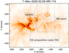 |
Fig. 1. HRIEUV image of the full field of view. The three highlighted boxes show the location of the EIS field of view during the Solar Orbiter observing campaign, the EIS field of view for the composition raster on 6 March 2022 at 23:26 UT, and a zoom in of the dynamical loops used later in this work. The image is displayed in a reverse colour scale (i.e. red coloured patches indicate bright regions on the Sun). |
Hinode (Kosugi et al. 2007) EIS (Culhane et al. 2007) was also observing this active region. In this work, we explore the upflow region, and with the new datasets from HRIEUV, we characterise the coronal activity in this region. We used EIS data from two separate studies. The first overlapped in time with the HRIEUV observation period and observed the persistent coronal upflows. The second EIS data was from just before the start of the HRIEUV, and it had enough spectral lines to determine the composition. The field of views of the EIS observations can be seen in Fig. 1. During the HRIEUV observing period, EIS operated in a raster mode, using the raster el_dhb_raster1. The raster duration was just under 4 min and the 2″ slit was used. This study was run during the full duration of the HRIEUV high-cadence observation started on 7 March 2022 at 00:05 UT and finished on 7 March 2022 at 02:02 UT. The EIS data were calibrated using the IDL SolarSoft routine eis_prep and the updated radiometric calibration of Warren et al. (2014). A single Gaussian fit was applied to the Fe XII emission line data in order to determine the Doppler velocities. The mean value of the fitted line centroids in the raster was used as the rest wavelength. The Doppler velocities were not corrected for the position on the disc. We used the Doppler velocities to identify upflow regions only and did not use the magnitude of the speeds for any extended analysis.
To measure the plasma composition, we used a different study (Atlas_30) that scans an area of 120″ × 160″ using the 2″ slit for around 33 min. This observation was made on 6 March 2022, starting at 23:26 UT. From this time until the end of the measurement made during the observing campaign with Solar Orbiter, the upflow region persisted. For the measurement, we used the Si X 258.375 Å to S X 264.223 Å abundance diagnostic. We took into account the temperature and density sensitivity of the ratio as follows. First, we determined the plasma density using the Fe XIII 202.044/203.826 diagnostic ratio. Then, we established the atmospheric temperature structure (differential emission measure – DEM) using a Markov chain Monte Carlo (MCMC) code. For the DEM calculation, we used the Fe line intensities shown in Table 1.
Fe emission lines used in the DEM analysis.
To account for possible cross-detector calibration issues, we adjusted the Fe DEM to match the Si X 258.375 Å line intensity. With the density and temperature structure known, we modelled the S X 264.223 Å intensity assuming photospheric abundances. The FIP effect enhances the abundances of elements with an FIP less than ∼10 eV. When no FIP effect is present, this procedure models the S X 264.223 Å intensity well. When the FIP effect is operating, however, the S X 264.223 Å intensity is too strong by a factor f, which is commonly referred to as the FIP bias.
More details of the procedure and DEM method are given in Brooks & Warren (2011) and Brooks et al. (2015). The MCMC code we used is from the PintOfAle software package (Kashyap & Drake 1998, 2000). The atomic data were taken from the CHIANTI database (Dere et al. 1997) version 10 (Del Zanna et al. 2021). We adopted the photospheric abundances from Scott et al. (2015a,b).
The Solar Dynamics Observatory (SDO) Atmospheric Imaging Assembly (AIA) data in 171 Å and 193 Å bands (Pesnell et al. 2012; Lemen et al. 2012) were used for context. We also analysed SDO/Helioseismic and Magnetic Imager (HMI; Scherrer et al. 2012) data that consist of line-of-sight (LOS) magnetograms selected from the full-disc data. We use magnetograms obtained with a temporal resolution of 45 s or 720 s, according to the analysis we performed, downloaded from the Joint Science Operation Center (JSOC1). We also used HMI pseudo-continuum images that provide white-light (WL) information at a rate of one frame every 45 s. In all cases, the magnetic data have a pixel resolution of 0.5″. The EIS intensity data for 195 Å was aligned to the AIA 193 Å filter. The AIA 171 Å filter image was then aligned to HRIEUV.
3. Results
The coronal upflow region in the active region we studied is not at the periphery, as is normally seen, but is instead close to the umbra. So the physical process(es) that created the upflow is likely different than when the upflow is observed at the edge of an active region. Figure 2 shows the EIS data for the Fe XII emission line with intensity and Doppler velocity. In the figure, a distinct upflow region can be seen in the EIS data (seen as blue in the bottom right panel). The AIA 193 Å image and the HMI magnetic field data are also shown with a larger field of view for context. The upflows are located in the penumbra region. They are not located around the whole penumbra but only in the region associated with small opposite polarity (positive) magnetic fragments. The rest of the penumbra has red-shifts around the rest of the sunspot. The umbra itself has a mix of blue and red-shifts and can be clearly seen in the coronal intensity images as the region with the lowest intensity (bright in the reversed colour table of Fig. 2).
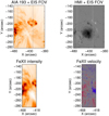 |
Fig. 2. FOVs of AIA, HMI and EIS. Top-left panel: AIA 193 image with the box showing the EIS field of view (reverse colour table). Top-right panel: HMI data with a range of ±2000 G. The white lines indicate the EIS field of view. Bottom-left panel: intensity of Fe XII (195.12 Å) in EIS (reverse colour table). Bottom-right panel: Doppler velocity of Fe XII with a range from −30 to +30 km s−1. The colours indicated red-shift (red) and blue-shift (blue). |
The high spatial resolution data from HRIEUV allowed us to explore this unusual upflow region further. Figure 3 shows a zoom in of the HRIEUV field of view with the Fe XII Doppler velocity shown as contours. The upflow region is located at the edge of small-scale loops and in the penumbra. Figure 3 also shows that these short loops are connected to small-scale positive polarity magnetic fragments. The umbra and penumbra have strong negative polarity field values. The rest of the coronal material surrounding the umbra is in the form of long loops or fibrils. The short loops associated with the upflows are extremely dynamic. Unfortunately, the EIS field of view does not show the full extent of these small loops, and we only saw the end of one loop.
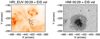 |
Fig. 3. Left panel: HRIEUV image (reverse colour table) with contours from the EIS Doppler velocity of the Fe XII emission lines. The contours shown are for velocities for −10 km s−1. Right panel: photospheric continuum data from HMI with the same EIS Doppler velocity contour. A movie (HRI_movie.mov) associated with this figure is available online. |
3.1. Investigating the activity around the active region using HRIEUV
To examine the activity levels in different areas of the active region, multiple artificial slits were placed along different structures, and space-time plots (or stack plots) were produced, which are shown in Fig. 4. In the figure, Slit 3 is the region where we found the upflow and the dynamic opposite polarity fragments. The bright parabolic-like tracks in Slit 1 and Slit 2 stack plots are basically EUV signatures of dynamic fibrils, which appear as small bright blobs moving back and forth with time (Mandal et al. 2023). These blobs are likely to be the tip of chromospheric fibrils that are shock driven phenomena (e.g. Hansteen et al. 2006). Slits 4 and 5 show propagating disturbances along long fan loops (e.g. Krishna Prasad et al. 2012). Slit 3, which lies within our region of interest, shows a different behaviour with time. Along this slit, there are multiple bright features that brighten and fade. However, there is no clear propagation or movement of these bright structures (i.e. there are no obvious bright parabolic tracks here). The different loops that appear and disappear can be seen clearly in the online movie associated with Fig. 3. We also note that Slit 3 has an upflow region associated with it, whereas the other slits do not.
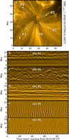 |
Fig. 4. Stack plots in different locations around the active region. Top panel a: HRIEUV image with artificial slits (white boxes) overlaid on it. Bottom panels b–f: Space-time plots derived using the artificial slits in panel a. The regions with Slits 1 and 2 behave like dynamic fibrils, while Slits 5 and 4 have propagating disturbances. Slit 3, which resides within the blue-shifted feature we noted earlier, shows multiple small bright features that change with time. An animated version of this figure is available online. |
To explore the dynamics further, we took a slice across the loops (see Fig. 5). We observed that loops brighten and fade on short timescales of only minutes. Such short timescales could also explain the photospheric abundance. The plasma was not confined in the corona long enough to reach coronal abundances.
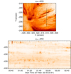 |
Fig. 5. Stack plot of the HRIEUV data across the small dynamic loops. Top panel: zoom in of the HRIEUV image focusing on the small-scale loops related to the upflows. A reverse colour table is used. Lower panel: stack plot with the y-axis at the position along the slit in arcsec across the loops to illustrate the dynamics. The x-axis shows time. The loops brighten and fade within only minutes. |
3.2. Dynamics and composition using EIS
Figure 6 shows the EIS intensity and Doppler velocity maps for Fe XI–XV. The boxes on the Fe XII maps highlight the two regions of strong Doppler velocity, one of which is red-shifted (R2), and the other is the blue-shifted region already discussed (R1). Upflow regions at the edges of active regions often have coronal composition. Measurements of elemental abundances above the umbra were found to indicate photospheric composition (Baker et al. 2021). In our analysis, the composition in the upflow region is also photospheric, with a FIP bias of 1.1. The downflow (red-shifted) region shows a coronal FIP bias of ≈2. The measurements of the non-thermal velocities (not shown here) are an indication of how turbulent the plasma is, suggesting that the largest non-thermal velocity is in the upflow region, with a much weaker one in the region of the downflows. The FIP bias values for these regions are also shown in Table 2, along with the observed intensities, calculated intensities, and differences between them for the Fe lines used in the DEM analysis. The latter gives an indication of the accuracy of the DEM and FIP bias calculation. For the measurements shown here, 85% of the line intensities were reproduced within ≈25% of the original intensity measurements.
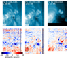 |
Fig. 6. EIS intensity (top) and Doppler velocity (bottom) maps as a function of increasing temperature (from left to right) for the raster used to measure the composition on 6 March 2022 23:26. The Fe XII 195.119 Å line here is deblended from the density sensitive 195.18 Å line. The data are resampled to an arcsec scale. The box (R3) on the Fe XI 188.216 Å intensity map shows where the composition measurement was made in the sunspot umbra. The boxes on the Fe XII 195.119 Å maps show the locations where the plasma composition measurements were made in the unusual blue-shifted upflow on the sunspot umbra (R1) and the red-shifted active region loops (R2). The Fe XV 284.160 Å image has been shifted upwards to account for the offset between the short- and long-wavelength detectors. |
3.3. Magnetic fields related to the upflow regions
Figure 7 shows a zoom in of the region containing the upflows with the magnetic field data overlaid. The upflows are at the edge of the series of small loops that connect the umbra to the positive polarity small magnetic fragments. These small magnetic fragments fluctuate (see the next paragraph on the magnetic field evolution), and the loops are extremely dynamic (see HRI_HMI movie). During the observing period, small loops were always in this region. They brightened and faded in timescales of minutes. Also during this time, the upflow region persisted. Its maximum blue-shifts in each raster are between −27 km s−1 and −19 km s−1.
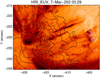 |
Fig. 7. HRIEUV image zoomed in on the region with the coronal upflows shown with a reverse colour table. The contours show the HMI magnetic field with the white colour showing positive polarity and black showing negative polarity (±2000 G). A movie (HRI_HMI.mov) associated with this figure is available online. |
Next we explore the magnetic field and continuum evolution of the negative spot and concentrate on where the upflows were observed. AR 12960 consisted of a concentrated leading negative polarity spot followed by more dispersed positive spots. Throughout its disc transit, the active region was seen to decay, as evidenced by the presence of an extended moat around the main negative polarity. Moat regions (see van Driel-Gesztelyi & Green 2015, and references therein), which are mostly seen around evolved and decaying spots, play a key role in transporting flux away from the active region and contributing to their decay. The evolution of the moat region is visible in the online movie accompanying this article (HMI-20220307e.mpeg). This moat region extends along the high-resolution observations of HRIEUV. The two left panels of Fig. 8 show the leading negative spot surrounded by a part of the moat region. Small magnetic features, called moving magnetic features (MMFs; Harvey & Harvey 1973), can be seen to move away from all sides of the spot. Towards the west, at the location of the upflow region, the negative polarity fragments cancel the flux of an elongated positive polarity, where we speculate the short dynamic loops are anchored in the penumbra end. The top-right panel of the figure illustrates the decrease of the positive polarity flux around 21:00 UT on 7 March. The positive flux has almost disappeared and, similarly, so has the connectivity represented by the short dynamic loops. We also analysed HMI continuum images (see the bottom-right panel of Fig. 8), whose evolution can be followed in the accompanying online movie (IC-20220307d.mpeg). Dark grains moving along the penumbral fibrils are noticeable only at the location of the upflows in the movie (see Sobotka & Puschmann 2022, who discussed grain motions along penumbral fibrils). As evident from both the magnetic field and continuum evolution, the region where the upflows are observed at the coronal level is also highly dynamic at the photospheric level, which could contribute to their formation.
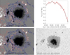 |
Fig. 8. Evolution of the magnetic field. Left panels: evolution of the moat region surrounding the leading negative spot between 00:07:56 UT and 02:52:56 UT on 7 March 2022. This range of time covers the HRIEUV high-resolution observation time. MMFs can be seen in both panels. The magnetic field values have been saturated above (below) 800 G (−800 G). The size of the panels is 250 × 200 pixels. We added three isocontours of the LOS field corresponding to ±30, ±100, and ±800 G, outlined in red (blue) style for the positive (negative) values. A movie with a similar field of view and similar saturation is associated with these panels. Magnetograms in this movie were taken every 3 min. Top-right panel: magnetic flux decrease of the elongated positive polarity to the west of the spot in the same time range as the left panels. The red line corresponds to one magnetic field measurement every 3 min, while the black line represents a smoothing every 4 points. This positive polarity is the site where the western footpoints of the short dynamic loops seen by HRIEUV could be located (see also Fig. 10). Bottom-right panel: HMI continuum image at 02:52:56 UT. A few dark grains can be seen along the penumbral filaments at the location of the upflow region. These grains are seen in motion in the movie associated with this panel. We also note the presence of light bridges in the umbra, which are typical of decaying sunspots. Two movies associated with this figure are available online. The first shows the magnetogram (HMI-20220307e.mpeg), and the second shows the continuum (IC-20220307d.mpeg). |
3.4. Magnetic field modelling
To understand what could be physically causing the photospheric abundance in the upflow region, we carried out a local magnetic field model of AR 12960. Figure 9 shows the coronal structure derived from our modelling for which we used the closest in time LOS HMI magnetogram to the start of HRIEUV observations as boundary a condition. The figure was constructed by superposing field lines computed using different linear-force-free field (LFFF) models, that is, ∇ × B = αB, where B is the magnetic field and α is a constant (see Mandrini et al. 2015, and references therein for a description of the model and its limitations). The free parameter of each of our models, α, was selected to better match the shape of the observed loops in AIA 171 Å (see the procedure discussed in Green 2002). For this comparison, the model was first transformed from the local frame to the observed frame, as discussed in Mandrini et al. (2015). This allowed a direct comparison of the computed coronal field configuration to the AIA image obtained at a similar time and shown as background in Fig. 9. Figure 10 shows a zoom concentrated on the western region of the leading sunspot. In this figure, a set of short field lines, in blue, has been computed starting from the integration in the sunspot penumbra where the eastern end of the short dynamic loops could be. These lines have their opposite footpoints in the elongated positive polarity located to the west of the spot, and they represent the observed short loops. We also computed a set of large-scale field lines with footpoints closer to the umbra. These lines extend farther out of our integration box and can be considered as “open” in our local model. Considering the location of their eastern footpoints, both sets of field lines (short and large-scale) could contain the upflowing plasma with the photospheric abundance we determined.
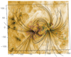 |
Fig. 9. Magnetic field model of AR 12960 on 7 March overlaid on an AIA 171 Å image with the intensity reversed. The axes in the panel are labelled in Megametres, with the origin set in the active region centre. The isocontours of the LOS field correspond to ±30, ±100, and ±800 G outlined in magenta (cyan) style for the positive (negative) values. Sets of computed field lines matching the global shape of the observed coronal loops are indicated with black lines. |
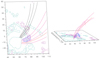 |
Fig. 10. Magnetic field models for the active region. Left panel: zoom of the magnetic field model of AR 12960 with sets of computed lines starting at integration in the umbral and penumbral region to the west of the preceding sunspot. The blue lines correspond to the short dynamic loops observed with HRIEUV. The red lines anchored in the umbra correspond to large-scale loops; these lines reach the border of the integration box. The set of black lines were added to show the change in connectivity. Right panel: same set of field lines shown in the left panel (except the black set) but from a different perspective. This image illustrates the relation between short- and large-scale structures. The height of the field lines has been arbitrarily multiplied by a factor of three for better visibility. The convention for isocontours and axes labels is the same as for Fig. 9. |
To explore if it is possible for the plasma in the large-scale lines shown in Fig. 10 to flow into the solar wind, we constructed a global potential-field source-surface (PFSS) model. Starting on 7 March 2022, Carrington Rotation (CR) 2255 contained the active region of interest. The corresponding HMI synoptic map is the boundary condition for our global PFSS model. We used the Finite Difference Iterative Potential-Field Solver (FDIPS) code developed by Tóth et al. (2011) 2, which solves the Laplace equation in an adaptive spherical grid. In this particular case, we used a grid with 360 grid points for longitude (spatial resolution of one), 180 for latitude (0.011 in the sine of latitude), and 150 grid points for the radial direction (spatial resolution of 0.01). We also set the source surface at a height of 2.5 R⊙, at which all magnetic field lines become radial. Figure 11 shows the extrapolation of a set of magnetic field lines covering AR 12960 and its neighbourhood. The red lines highlight open magnetic fields anchored in negative polarities, and the black lines show closed lines. The red lines anchored in the negative polarity sunspot of AR 12960 correspond to our large-scale lines reaching the integration box in the local model. The figure depicts three different viewpoints to understand the magnetic morphology around the active region. A pseudo-streamer is seen above AR 12960, the western open lines allow a clear path of the upflowing plasma into the solar wind.
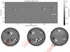 |
Fig. 11. PFSS model carried out for CR 2255. Top panel: corresponding HMI synoptic map. AR 12960 is located at a longitude of 340° and a latitude of −20°. Lower panels: three different points of view of the PFSS model illustrating the existence of a pseudo-streamer. The right view point corresponds to a solar disc centre located at 330° of longitude and 0° of latitude. The middle view point remains at the same latitude but sets the solar disc centre at a longitude of 360°. The left view point has the solar disc centre at a latitude of 50° and a longitude of 360°. The black lines correspond to closed field lines, and the red lines denote open field lines anchored in negative field polarities. The bar to the right of the top panel indicates the scale of the magnetic field values. |
We also tried to link the remote sensing observations of the active region to the Solar Orbiter in situ measurements in order to compare plasma composition features with the Solar Wind Analyzer/Heavy Ion Sensor (SWA/HIS) data (Owen et al. 2020). By utilising the Magnetic Connectivity Tool3 (‘MCT’) developed by Rouillard et al. (2020), we identified time periods of potential magnetic connection between AR 12960 and the Solar Orbiter spacecraft. In principle, such a predicted connection would allow outflowing solar wind plasma to be measured in situ by the SWA sensors in the following days. The slow solar wind emitted from AR 12960 on the beginning of 7 March arrives to the Solar Orbiter in the early hours of 9 March, assuming a radial propagation with constant speed from the source surface out to 0.5 AU. During 8 and 9 March, the MCT predicts an occasional magnetic connection between Solar Orbiter and the close vicinity of AR 12960. However, it also yields quite large uncertainties during the same time period, as indicated by two different predicted source regions in the utilised Air Force Data Assimilative Photospheric Flux Transport (ADAPT) model (Hickmann et al. 2015) that are separated by 60° in solar longitude. Additionally, in the Solar Orbiter in situ plasma data, we observed a clear signature of passing interplanetary coronal mass ejections (ICMEs) with two extended flux rope structures in the interplanetary magnetic field (IMF) between 8 March and mid 9 March, which is likely to limit the applicability of the MCT tool during this time period. The signature of the passing ICMEs during 8 and 9 March is also visible through increased Fe/O abundance ratios, up to about 0.5 in the SWA/HIS data (not shown here). Unfortunately, it was not possible to link the in situ solar wind data with the remote sensing observations in this case.
4. Discussion and conclusions
In this work, we analysed an active region (NOAA 12960) that was observed during the first Solar Orbiter perihelion. The joint observing campaign between Hinode and the Solar Orbiter allowed for spectroscopic analysis of coronal emission lines along with high time cadence and high spatial resolution observations in the corona from HRIEUV. We were particularly interested in the upflow area of the active region due to the potential of flows flowing from the active region into the slow solar wind.
Previous observations have shown upflows at the edges of active regions. The flows are persistent and long lasting. In this active region, we observed the strongest upflows close to the umbra in a region that is connected to small opposite polarity fragments. Our analysis shows that this region has a photospheric FIP bias instead of the coronal FIP bias that is usually seen in the upflow regions at the edges of active regions.
The FIP and anti-FIP effects were well observed in the Sun at different locations as well as in other stars. This effect is summarised well by Laming (2015). As mentioned in the introduction, the closed loop corona and slow solar wind show an enhanced abundance of elements with low FIP (< 10 eV) relative to the photosphere, whereas the high FIP elements (> 10 eV) do not change. However, the increase for the low FIP elements is not seen in coronal holes. One potential explanation for the different FIP biases observed is related to how forces associated with the reflection or refraction of Alfvèn waves in the chromosphere act on ions but not neutrals. This causes different fractionation in different locations for different elements, depending on the magnetic topology. The open magnetic field allows waves propagating from the photosphere to continue along the magnetic field with little resonance and hence little fractionation. In closed magnetic field lines, Laming (2015) suggests that resonant waves are excited by nanoflare reconnection creating enhanced fractionation of the plasma.
In the active region analysed in this work, the FIP bias was measured to be close to one, which indicates a photospheric composition. One possibility for this measurement is that the small-scale loops live for short periods of time (i.e. only a few minutes). They are highly dynamic and are also likely to be interacting with the large-scale loops that emanate from the umbra. As discussed in Baker et al. (2021), the umbra of a large sunspot has photospheric composition. In our case, the sunspot is smaller in size but also has photospheric abundances.
The physical cause of this upflow and composition is interesting. The magnetic modelling clearly shows small loops located next to the large-scale loops coming from the umbra in the small region of coronal upflow. However, the modelling does not show a clear opportunity for the type of interchange reconnection that was seen in Parenti et al. (2021), for example, which leads to mixed FIP biases being observed between the open and closed magnetic field interaction. The dynamics of the small loops that we studied were caused by the rapid cancellation of the small positive polarity magnetic flux. The loops are short-lived, giving little time for resonances of waves to develop; hence the FIP bias stays photospheric. In addition, the photosphere also shows movement of small grains at that same location.
In this paper, we have shown another – as well as different – source of coronal upflow in active regions. This is of particular interest because of the photospheric composition of the region. The slow solar wind can have a mix of compositions, and our results show a potential new source for photospheric composition in an active region. Our results emphasise the importance of small-scale magnetic fragments within an active region, as the fragments can have an impact on not only the dynamics of the plasma but also its composition.
Movies
Movie 1 associated with Fig. 3 (HMI-20220307e) Access here
Movie 2 associated with Fig. 4 (HRI_movie) Access here
Movie 3 associated with Fig. 7 (HRI_HMI) Access here
Movie 4 associated with Fig. 8 (IC-20220307d) Access here
The MCT is available as an online tool at http://connect-tool.irap.omp.eu/
Acknowledgments
The work of D.H.B. was performed under contract to the Naval Research Laboratory and was funded by the NASA Hinode program. S.P. acknowledges the funding by CNES through the MEDOC data and operations center. C.H.M. and G.C. acknowledge grants PICT-2020-SERIEA-03214, PIP 11220200100985, and UBACyT 20020170100611BA. G.C. is a member of the Carrera del Investigador Científico of the Consejo Nacional de Investigaciones Científicas y Técnicas (CONICET). C.H.M. is a Senior Researcher at CONICET. Hinode is a Japanese mission developed and launched by ISAS/JAXA, with NAOJ as domestic partner and NASA and STFC (UK) as international partners. It is operated by these agencies in cooperation with ESA and NSC (Norway). The SDO data are courtesy of NASA/SDO and the AIA, EVE, and HMI science teams. Solar Orbiter is a mission of international cooperation between ESA and NASA, operated by ESA. The EUI instrument was built by CSL, IAS, MPS, MSSL/UCL, PMOD/WRC, ROB, LCF/IO with funding from the Belgian Federal Science Policy Office (BELSPO/PRODEX) under contracts 4000134088, 4000112292, 4000134474, and 4000136424; the Centre National d’Études Spatiales (CNES); the UK Space Agency (UKSA); the Bundesministerium für Wirtschaft und Energie (BMWi) through the Deutsches Zentrum für Luft- und Raumfahrt (DLR); and the Swiss Space Office (SSO). A.C.S. was supported by NASA’s Heliophysics Supporting Research (HSR) and Heliophysics System Observatory Connect (HSOC) programs, and also by the NASA/MSFC Hinode Project.
References
- Abbo, L., Ofman, L., Antiochos, S. K., et al. 2016, Space Sci. Rev., 201, 55 [NASA ADS] [CrossRef] [Google Scholar]
- Baker, D., van Driel-Gesztelyi, L., Mandrini, C. H., Démoulin, P., & Murray, M. J. 2009, ApJ, 705, 926 [NASA ADS] [CrossRef] [Google Scholar]
- Baker, D., Stangalini, M., Valori, G., et al. 2021, ApJ, 907, 16 [Google Scholar]
- Berghmans, D., Auchère, F., Long, D. M., et al. 2021, A&A, 656, L4 [NASA ADS] [CrossRef] [EDP Sciences] [Google Scholar]
- Berghmans, D., Antolin, P., Auchère, F., et al. 2023, A&A, in press, https://doi.org/10.1051/0004-6361/202245586 (SO Nominal Mission Phase SI) [Google Scholar]
- Boutry, C., Buchlin, E., Vial, J. C., & Régnier, S. 2012, ApJ, 752, 13 [NASA ADS] [CrossRef] [Google Scholar]
- Brooks, D. H., & Warren, H. P. 2011, ApJ, 727, L13 [Google Scholar]
- Brooks, D. H., & Warren, H. P. 2012, ApJ, 760, L5 [NASA ADS] [CrossRef] [Google Scholar]
- Brooks, D. H., Ugarte-Urra, I., & Warren, H. P. 2015, Nat. Commun., 6, 5947 [Google Scholar]
- Brooks, D. H., Winebarger, A. R., Savage, S., et al. 2020, ApJ, 894, 144 [Google Scholar]
- Bryans, P., Young, P. R., & Doschek, G. A. 2010, ApJ, 715, 1012 [NASA ADS] [CrossRef] [Google Scholar]
- Culhane, J. L., Harra, L. K., James, A. M., et al. 2007, Sol. Phys., 243, 19 [Google Scholar]
- Culhane, J. L., Brooks, D. H., van Driel-Gesztelyi, L., et al. 2014, Sol. Phys., 289, 3799 [Google Scholar]
- Del Zanna, G. 2008, A&A, 481, L49 [NASA ADS] [CrossRef] [EDP Sciences] [Google Scholar]
- Del Zanna, G., Aulanier, G., Klein, K. L., & Török, T. 2011, A&A, 526, A137 [NASA ADS] [CrossRef] [EDP Sciences] [Google Scholar]
- Del Zanna, G., Dere, K. P., Young, P. R., & Landi, E. 2021, ApJ, 909, 38 [NASA ADS] [CrossRef] [Google Scholar]
- Démoulin, P., Henoux, J. C., Priest, E. R., & Mandrini, C. H. 1996, A&A, 308, 643 [Google Scholar]
- Dere, K. P., Landi, E., Mason, H. E., Monsignori Fossi, B. C., & Young, P. R. 1997, A&AS, 125, 149 [NASA ADS] [CrossRef] [EDP Sciences] [Google Scholar]
- Doschek, G. A., Warren, H. P., Mariska, J. T., et al. 2008, ApJ, 686, 1362 [NASA ADS] [CrossRef] [Google Scholar]
- Edwards, S. J., Parnell, C. E., Harra, L. K., Culhane, J. L., & Brooks, D. H. 2016, Sol. Phys., 291, 117 [Google Scholar]
- Feldman, U., & Widing, K. G. 2007, Space Sci. Rev., 130, 115 [CrossRef] [Google Scholar]
- Green, L. M., López fuentes, M. C., Mandrini, C. H., et al. 2002, Sol. Phys., 208, 43 [Google Scholar]
- Hansteen, V. H., De Pontieu, B., Rouppe van der Voort, L., van Noort, M., & Carlsson, M. 2006, ApJ, 647, L73 [Google Scholar]
- Harra, L. K., Sakao, T., Mandrini, C. H., et al. 2008, ApJ, 676, L147 [Google Scholar]
- Harvey, K., & Harvey, J. 1973, Sol. Phys., 28, 61 [Google Scholar]
- Hickmann, K. S., Godinez, H. C., Henney, C. J., & Arge, C. N. 2015, Sol. Phys., 290, 1105 [NASA ADS] [CrossRef] [Google Scholar]
- Kashyap, V., & Drake, J. J. 1998, ApJ, 503, 450 [Google Scholar]
- Kashyap, V., & Drake, J. J. 2000, Bull. Astron. Soc. India, 28, 475 [NASA ADS] [EDP Sciences] [Google Scholar]
- Kosugi, T., Matsuzaki, K., Sakao, T., et al. 2007, Sol. Phys., 243, 3 [Google Scholar]
- Krishna Prasad, S., Banerjee, D., & Singh, J. 2012, Sol. Phys., 281, 67 [NASA ADS] [Google Scholar]
- Laming, J. M. 2015, Liv. Rev. Sol. Phys., 12, 2 [Google Scholar]
- Lemen, J. R., Title, A. M., Akin, D. J., et al. 2012, Sol. Phys., 275, 17 [Google Scholar]
- Liewer, P. C., Neugebauer, M., & Zurbuchen, T. 2004, Sol. Phys., 223, 209 [NASA ADS] [CrossRef] [Google Scholar]
- Mampaey, B., Verbeeck, F., Stegen, K., et al. 2022, SolO/EUI Data Release 5.0 2022-04 [Google Scholar]
- Mandal, S., Peter, H., Chitta, L. P., et al. 2023, A&A, 670, L3 (SO Nominal Mission Phase SI) [NASA ADS] [CrossRef] [EDP Sciences] [Google Scholar]
- Mandrini, C. H., Nuevo, F. A., Vásquez, A. M., et al. 2014, Sol. Phys., 289, 4151 [NASA ADS] [CrossRef] [Google Scholar]
- Mandrini, C. H., Baker, D., Démoulin, P., et al. 2015, ApJ, 809, 73 [Google Scholar]
- Marsch, E., Tian, H., Sun, J., Curdt, W., & Wiegelmann, T. 2008, ApJ, 685, 1262 [NASA ADS] [CrossRef] [Google Scholar]
- McIntosh, S. W., Tian, H., Sechler, M., & De Pontieu, B. 2012, ApJ, 749, 60 [NASA ADS] [CrossRef] [Google Scholar]
- Müller, D., St. Cyr, O. C., Zouganelis, I., et al. 2020, A&A, 642, A1 [Google Scholar]
- Ofman, L., Wang, T. J., & Davila, J. M. 2012, ApJ, 754, 111 [NASA ADS] [CrossRef] [Google Scholar]
- Owen, C. J., Bruno, R., Livi, S., et al. 2020, A&A, 642, A16 [EDP Sciences] [Google Scholar]
- Parenti, S., Chifu, I., Del Zanna, G., et al. 2021, Space Sci. Rev., 217, 78 [NASA ADS] [CrossRef] [Google Scholar]
- Pesnell, W. D., Thompson, B. J., & Chamberlin, P. C. 2012, Sol. Phys., 275, 3 [Google Scholar]
- Peter, H. 2010, A&A, 521, A51 [NASA ADS] [CrossRef] [EDP Sciences] [Google Scholar]
- Rochus, P., Auchère, F., Berghmans, D., et al. 2020, A&A, 642, A8 [NASA ADS] [CrossRef] [EDP Sciences] [Google Scholar]
- Rouillard, A. P., Pinto, R. F., Vourlidas, A., et al. 2020, A&A, 642, A2 [NASA ADS] [CrossRef] [EDP Sciences] [Google Scholar]
- Sakao, T., Kano, R., Narukage, N., et al. 2007, Science, 318, 1585 [NASA ADS] [CrossRef] [Google Scholar]
- Scherrer, P. H., Schou, J., Bush, R. I., et al. 2012, Sol. Phys., 275, 207 [Google Scholar]
- Scott, P., Grevesse, N., Asplund, M., et al. 2015a, A&A, 573, A25 [NASA ADS] [CrossRef] [EDP Sciences] [Google Scholar]
- Scott, P., Asplund, M., Grevesse, N., Bergemann, M., & Sauval, A. J. 2015b, A&A, 573, A26 [NASA ADS] [CrossRef] [EDP Sciences] [Google Scholar]
- Sobotka, M., & Puschmann, K. G. 2022, A&A, 662, A13 [NASA ADS] [CrossRef] [EDP Sciences] [Google Scholar]
- Tian, H., McIntosh, S. W., De Pontieu, B., et al. 2011, ApJ, 738, 18 [NASA ADS] [CrossRef] [Google Scholar]
- Tian, H., McIntosh, S. W., Wang, T., et al. 2012, ApJ, 759, 144 [Google Scholar]
- Tian, H., Harra, L., Baker, D., Brooks, D. H., & Xia, L. 2021, Sol. Phys., 296, 47 [NASA ADS] [CrossRef] [Google Scholar]
- Tóth, G., van der Holst, B., & Huang, Z. 2011, ApJ, 732, 102 [CrossRef] [Google Scholar]
- van Driel-Gesztelyi, L., & Green, L. M. 2015, Liv. Rev. Sol. Phys., 12, 1 [Google Scholar]
- van Driel-Gesztelyi, L., Culhane, J. L., Baker, D., et al. 2012, Sol. Phys., 281, 237 [Google Scholar]
- Verwichte, E., Marsh, M., Foullon, C., et al. 2010, ApJ, 724, L194 [NASA ADS] [CrossRef] [Google Scholar]
- von Steiger, R., Schwadron, N. A., Fisk, L. A., et al. 2000, J. Geophys. Res., 105, 27217 [Google Scholar]
- Warren, H. P., Ugarte-Urra, I., Young, P. R., & Stenborg, G. 2011, ApJ, 727, 58 [NASA ADS] [CrossRef] [Google Scholar]
- Warren, H. P., Ugarte-Urra, I., & Landi, E. 2014, ApJS, 213, 11 [NASA ADS] [CrossRef] [Google Scholar]
- Young, P. R., O’Dwyer, B., & Mason, H. E. 2012, ApJ, 744, 14 [NASA ADS] [CrossRef] [Google Scholar]
- Zurbuchen, T. H., von Steiger, R., Gruesbeck, J., et al. 2012, Space Sci. Rev., 172, 41 [NASA ADS] [CrossRef] [Google Scholar]
All Tables
All Figures
|
Fig. 1. HRIEUV image of the full field of view. The three highlighted boxes show the location of the EIS field of view during the Solar Orbiter observing campaign, the EIS field of view for the composition raster on 6 March 2022 at 23:26 UT, and a zoom in of the dynamical loops used later in this work. The image is displayed in a reverse colour scale (i.e. red coloured patches indicate bright regions on the Sun). |
| In the text | |
|
Fig. 2. FOVs of AIA, HMI and EIS. Top-left panel: AIA 193 image with the box showing the EIS field of view (reverse colour table). Top-right panel: HMI data with a range of ±2000 G. The white lines indicate the EIS field of view. Bottom-left panel: intensity of Fe XII (195.12 Å) in EIS (reverse colour table). Bottom-right panel: Doppler velocity of Fe XII with a range from −30 to +30 km s−1. The colours indicated red-shift (red) and blue-shift (blue). |
| In the text | |
|
Fig. 3. Left panel: HRIEUV image (reverse colour table) with contours from the EIS Doppler velocity of the Fe XII emission lines. The contours shown are for velocities for −10 km s−1. Right panel: photospheric continuum data from HMI with the same EIS Doppler velocity contour. A movie (HRI_movie.mov) associated with this figure is available online. |
| In the text | |
|
Fig. 4. Stack plots in different locations around the active region. Top panel a: HRIEUV image with artificial slits (white boxes) overlaid on it. Bottom panels b–f: Space-time plots derived using the artificial slits in panel a. The regions with Slits 1 and 2 behave like dynamic fibrils, while Slits 5 and 4 have propagating disturbances. Slit 3, which resides within the blue-shifted feature we noted earlier, shows multiple small bright features that change with time. An animated version of this figure is available online. |
| In the text | |
|
Fig. 5. Stack plot of the HRIEUV data across the small dynamic loops. Top panel: zoom in of the HRIEUV image focusing on the small-scale loops related to the upflows. A reverse colour table is used. Lower panel: stack plot with the y-axis at the position along the slit in arcsec across the loops to illustrate the dynamics. The x-axis shows time. The loops brighten and fade within only minutes. |
| In the text | |
|
Fig. 6. EIS intensity (top) and Doppler velocity (bottom) maps as a function of increasing temperature (from left to right) for the raster used to measure the composition on 6 March 2022 23:26. The Fe XII 195.119 Å line here is deblended from the density sensitive 195.18 Å line. The data are resampled to an arcsec scale. The box (R3) on the Fe XI 188.216 Å intensity map shows where the composition measurement was made in the sunspot umbra. The boxes on the Fe XII 195.119 Å maps show the locations where the plasma composition measurements were made in the unusual blue-shifted upflow on the sunspot umbra (R1) and the red-shifted active region loops (R2). The Fe XV 284.160 Å image has been shifted upwards to account for the offset between the short- and long-wavelength detectors. |
| In the text | |
|
Fig. 7. HRIEUV image zoomed in on the region with the coronal upflows shown with a reverse colour table. The contours show the HMI magnetic field with the white colour showing positive polarity and black showing negative polarity (±2000 G). A movie (HRI_HMI.mov) associated with this figure is available online. |
| In the text | |
|
Fig. 8. Evolution of the magnetic field. Left panels: evolution of the moat region surrounding the leading negative spot between 00:07:56 UT and 02:52:56 UT on 7 March 2022. This range of time covers the HRIEUV high-resolution observation time. MMFs can be seen in both panels. The magnetic field values have been saturated above (below) 800 G (−800 G). The size of the panels is 250 × 200 pixels. We added three isocontours of the LOS field corresponding to ±30, ±100, and ±800 G, outlined in red (blue) style for the positive (negative) values. A movie with a similar field of view and similar saturation is associated with these panels. Magnetograms in this movie were taken every 3 min. Top-right panel: magnetic flux decrease of the elongated positive polarity to the west of the spot in the same time range as the left panels. The red line corresponds to one magnetic field measurement every 3 min, while the black line represents a smoothing every 4 points. This positive polarity is the site where the western footpoints of the short dynamic loops seen by HRIEUV could be located (see also Fig. 10). Bottom-right panel: HMI continuum image at 02:52:56 UT. A few dark grains can be seen along the penumbral filaments at the location of the upflow region. These grains are seen in motion in the movie associated with this panel. We also note the presence of light bridges in the umbra, which are typical of decaying sunspots. Two movies associated with this figure are available online. The first shows the magnetogram (HMI-20220307e.mpeg), and the second shows the continuum (IC-20220307d.mpeg). |
| In the text | |
|
Fig. 9. Magnetic field model of AR 12960 on 7 March overlaid on an AIA 171 Å image with the intensity reversed. The axes in the panel are labelled in Megametres, with the origin set in the active region centre. The isocontours of the LOS field correspond to ±30, ±100, and ±800 G outlined in magenta (cyan) style for the positive (negative) values. Sets of computed field lines matching the global shape of the observed coronal loops are indicated with black lines. |
| In the text | |
|
Fig. 10. Magnetic field models for the active region. Left panel: zoom of the magnetic field model of AR 12960 with sets of computed lines starting at integration in the umbral and penumbral region to the west of the preceding sunspot. The blue lines correspond to the short dynamic loops observed with HRIEUV. The red lines anchored in the umbra correspond to large-scale loops; these lines reach the border of the integration box. The set of black lines were added to show the change in connectivity. Right panel: same set of field lines shown in the left panel (except the black set) but from a different perspective. This image illustrates the relation between short- and large-scale structures. The height of the field lines has been arbitrarily multiplied by a factor of three for better visibility. The convention for isocontours and axes labels is the same as for Fig. 9. |
| In the text | |
|
Fig. 11. PFSS model carried out for CR 2255. Top panel: corresponding HMI synoptic map. AR 12960 is located at a longitude of 340° and a latitude of −20°. Lower panels: three different points of view of the PFSS model illustrating the existence of a pseudo-streamer. The right view point corresponds to a solar disc centre located at 330° of longitude and 0° of latitude. The middle view point remains at the same latitude but sets the solar disc centre at a longitude of 360°. The left view point has the solar disc centre at a latitude of 50° and a longitude of 360°. The black lines correspond to closed field lines, and the red lines denote open field lines anchored in negative field polarities. The bar to the right of the top panel indicates the scale of the magnetic field values. |
| In the text | |
Current usage metrics show cumulative count of Article Views (full-text article views including HTML views, PDF and ePub downloads, according to the available data) and Abstracts Views on Vision4Press platform.
Data correspond to usage on the plateform after 2015. The current usage metrics is available 48-96 hours after online publication and is updated daily on week days.
Initial download of the metrics may take a while.