| Issue |
A&A
Volume 675, July 2023
BeyondPlanck: end-to-end Bayesian analysis of Planck LFI
|
|
|---|---|---|
| Article Number | A8 | |
| Number of page(s) | 9 | |
| Section | Cosmology (including clusters of galaxies) | |
| DOI | https://doi.org/10.1051/0004-6361/202243138 | |
| Published online | 28 June 2023 | |
BEYONDPLANCK
VIII. Efficient sidelobe convolution and corrections through spin harmonics
1
Institute of Theoretical Astrophysics, University of Oslo, Blindern, Oslo, Norway
e-mail: mathew.galloway@astro.uio.no
2
Max-Planck-Institut für Astrophysik, Karl-Schwarzschild-Str. 1, 85741 Garching, Germany
3
Dipartimento di Fisica, Università degli Studi di Milano, Via Celoria, 16, Milano, Italy
4
INAF-IASF Milano, Via E. Bassini 15, Milano, Italy
5
INFN, Sezione di Milano, Via Celoria 16, Milano, Italy
6
INAF – Osservatorio Astronomico di Trieste, Via G.B. Tiepolo 11, Trieste, Italy
7
Planetek Hellas, Leoforos Kifisias 44, Marousi, 151 25
Greece
8
Department of Astrophysical Sciences, Princeton University, Princeton, NJ, 08544
USA
9
Jet Propulsion Laboratory, California Institute of Technology, 4800 Oak Grove Drive, Pasadena, CA, USA
10
Department of Physics, Gustaf Hällströmin katu 2, University of Helsinki, Helsinki, Finland
11
Helsinki Institute of Physics, University of Helsinki, Gustaf Hällströmin katu 2, Helsinki, Finland
12
Computational Cosmology Center, Lawrence Berkeley National Laboratory, Berkeley, CA, USA
13
Haverford College Astronomy Department, 370 Lancaster Avenue, Haverford, PA, USA
14
Dipartimento di Fisica, Università degli Studi di Trieste, Via A. Valerio 2, Trieste, Italy
Received:
17
January
2022
Accepted:
18
March
2022
We introduce a new formulation of the Conviqt convolution algorithm in terms of spin harmonics, and apply this to the problem of sidelobe correction for BEYONDPLANCK, the first end-to-end Bayesian Gibbs sampling framework for CMB analysis. We compare our implementation to the previous Planck LevelS implementation, and find good agreement between the two codes in terms of accuracy, but with a speed-up reaching a factor of 3–10, depending on the frequency bandlimits, lmax and mmax. The new algorithm is significantly simpler to implement and maintain, since all low-level calculations are handled through an external spherical harmonic transform library. We find that our mean sidelobe estimates for Planck LFI are in good agreement with previous efforts. Additionally, we present novel sidelobe rms maps that quantify the uncertainty in the sidelobe corrections due to variations in the sky model.
Key words: cosmic background radiation / cosmology: observations
© The Authors 2023
 Open Access article, published by EDP Sciences, under the terms of the Creative Commons Attribution License (https://creativecommons.org/licenses/by/4.0), which permits unrestricted use, distribution, and reproduction in any medium, provided the original work is properly cited.
This article is published in open access under the Subscribe to Open model. Subscribe to A&A to support open access publication.
1. Introduction
Among the most important systematic effects that must be accounted for when observing the cosmic microwave background (CMB) are stray light and sidelobes (e.g., Barnes et al. 2003; Planck Collaboration III 2014). These effects come from the non-zero response of the detector to areas of the sky outside the main beam, however that may be defined for each particular case. Because microwave telescopes typically work near their diffraction limit, the presence of a certain extent of sidelobe effects is inevitable. Furthermore, their structure can be complicated by many different physical effects, such as spurious optical reflections or manufacturing irregularities in the detectors or optical elements. These signal contributions can have far-reaching consequences on the observed signal, particularly at large angular scales, as they do not behave in the same sky-stationary manner as the main beam signal.
Sidelobe signals can produce many types of errors in CMB analysis pipelines and they represent a potent source of systematic contamination (e.g., Planck Collaboration III 2016; Watts et al. 2023). In particular, as the sidelobe response functions often are broadly distributed, this contamination can confuse important signals such as the CMB solar and orbital dipoles that are used for calibration. Sidelobes uncertainties are coupled directly with foreground emission from diffuse galactic components, producing a significant source of contamination. In some experiments a further contaminating signal can originate from a source not on the sky, such as ground pickup or radio-frequency (RF) noise. In all cases, sidelobe signals are detrimental to the quality of the final sky maps and parameter estimates, and a dedicated effort is required to remove them. The process of characterizing and correcting these spurious signals is therefore an important part of optimal CMB mapmaking, and it requires optimized algorithms to do so efficiently. One of the most important of these steps is to convolve a beam or sidelobe response function with a sky map or model to generate a re-observed map.
Full-sky convolution on the sphere is a problem that has been important in the CMB field since the earliest satellite measurements. Early experiments like COBE (Toral et al. 1989) either did not model the sidelobes or they used simple pixel-based convolution approaches that (even at low resolution) still required radially symmetric beam approximations (Wu et al. 2001), or limited the applications to large scales (Burigana et al. 2001).
Wandelt & Górski (2001) presented the first harmonic space convolution algorithm, often referred to as “total convolution”, which achieved a large performance gain over pixel-based methods, by as much as a factor of  . This breakthrough allowed for the calculation of these convolutions easily enough that they could be applied to each simulation, instead of requiring a dedicated study necessitating months of runtime.
Next, Prézeau & Reinecke (2010) developed the Conviqt approach, which was used both by several official Planck analysis pipelines (Planck Collaboration III 2016, Planck Collaboration Int. XLVI 2016, Planck Collaboration Int. LVII 2020) and to generate the Planck Full Focal Plane (FFP) simulations (Planck Collaboration XII 2016). This approach was an improvement over the state of the art, speeding up the computation of the Wigner recursion relationships used in the original harmonic space algorithm, as well as providing a standardized, user-friendly library, libconviqt, which could be incorporated into numerous pipelines.
In this paper, we introduce a new formulation of the Conviqt algorithm that is based on spherical harmonic transforms (SHTs), rather than directly computing the Wigner matrix elements. We are thus able to leverage the highly optimized libsharp SHT library to perform the bulk of the calculations (Reinecke & Seljebotn 2013). Although this new approach was not developed specifically for BEYONDPLANCK, this paper is the first to explicitly derive, discuss, and benchmark the method.
2. Sidelobes, libconviqt, and libsharp
2.1. Total convolution through spin harmonics
Based on a given sky map,  , and beam,
  , our task is to compute a quantity c(ϑ, φ, ψ) ∈ ℝ that represents the convolution of these two fields, with the beam oriented in polar coordinates (ϑ, φ)1 and rotated around its own central axis by ψ,
Here, slms denotes the spherical harmonic coefficients of the sky signal and blmb is the beam in the same representation. In this expression, care must been taken to distinguish between the sky and beam bandlimits, ms and mb, as the two indices will be treated separately in the following derivation.
A computationally efficient solution for this problem was derived by Prézeau & Reinecke (2010), who exploited fast recurrence relations for Wigner d matrix elements to evaluate Eq. (1) in harmonic space. In the following, we show that this equation can alternatively be expressed in terms of spin-harmonics. The resulting algebra is in principle identical to the recursion relations used by Prézeau & Reinecke (2010), but the euqations are simply repackaged in a format that is significantly easier to implement in practical computer code, since it may use existing and highly optimized spherical harmonic libraries, such as libsharp (Reinecke & Seljebotn 2013), to perform the computationally expensive parts.
As shown by Wandelt & Górski (2001), Eq. (1) can be evaluated efficiently in harmonic space as
![$$ \begin{aligned} {c(\vartheta , \varphi , \psi )}= \sum _{l,m_s,m_b} s_{lm_s} b^*_{lm_b} [D^{l}_{m_sm_b}(\varphi ,\vartheta ,\psi )]^*, \end{aligned} $$](/articles/aa/full_html/2023/07/aa43138-22/aa43138-22-eq5.gif)
where slms and blmb are the spherical harmonic coefficients of the signal and beam, respectively, and  is the Wigner D-matrix.
This may be expressed as (Goldberg et al. 1967)
where sYlm(ϑ, φ) is the spin-weighted spherical harmonic and the placement of the negative signs are an arbitrary historical convention. Inserting this expression into Eq. (2) yields:
where we have assumed that the beam is real-valued in position space and we have used the symmetry relations:
![$$ \begin{aligned} D^l_{-m_s,-m_b}(\vartheta ,\varphi )&=(-1)^{m_s+m_b}[D^{l}_{m_s,m_b}(\vartheta ,\varphi )]^*, \end{aligned} $$](/articles/aa/full_html/2023/07/aa43138-22/aa43138-22-eq9.gif)
Pulling the summation over mb in front of the other sums yields
The terms in this outer sum can be arranged in the form mb = 0, ±1, ±2, …. The contribution from mb = 0 can be interpreted as a spin-0 spherical harmonic transform of the quantity  , which can be easily computed by a library such as libsharp (Reinecke & Seljebotn 2013).
Since c(ϑ, φ, ψ) ∈ ℝ, we know that the contributions from the pairs mb = ±1, ±2, … must be complex conjugate with respect to each other, and their combined contribution is therefore
![$$ \begin{aligned} e^{im_b\psi }_{m_b}&S(\vartheta ,\varphi ) + e^{-im_b\psi }_{m_b}S^*(\vartheta ,\varphi ) = \\\nonumber&2\left[\cos (m_b\psi )\text{ Re}(_{m_b}S(\vartheta ,\varphi )) - \sin (m_b\psi )\text{ Im}(_{m_b}S(\vartheta ,\varphi ))\right], \end{aligned} $$](/articles/aa/full_html/2023/07/aa43138-22/aa43138-22-eq13.gif)
where we have defined
This is a spherical harmonic transform of a quantity with a spin mb, which can also be computed efficiently by libsharp.
In practice, the transforms in Eq. (9) are implemented by separating S into its gradient and curl (or E and B) coefficients, alm (Lewis 2005):

using the symmetry relations  and
and 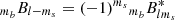 , and where the overall minus sign is a convention. Again making use of the symmetry relation in Eq. (6), this gives us:


To summarize, efficient evaluation of the convolution integral in Eq. (1) may be done through the following steps: Firstly, for each m = 0, …, mb, we pre-compute the spin spherical harmonic coefficients in Eqs. (11)–(12) and then compute the corresponding spin-mb SHT with an external library such as libsharp. This results in a three-dimensional data cube of the form c(ϑ, φ, mb). Then for each position on the sky, (ϑ, φ), we perform a Fourier transform to convert these coefficients to c(ϑ, φ, ψ), as given by Eq. (7).
In practice, the resulting c(ϑ, φ, ψ) data object is evaluated at a finite pixel resolution typically set to match the beam band limit. To obtain smooth estimates within this data object, a wide range of interpolation schemes may be employed, trading computational efficiency for accuracy. This issue is identical to what has been faced in previous approaches (Wandelt & Górski 2001; Prézeau & Reinecke 2010).
2.2. Comparison with libconviqt
To compare the results of this new total convolution approach with the older libconviqt approach of Prézeau & Reinecke (2010), we evaluated the convolution between the beam for one of the LFI 30 GHz receivers (28M) and a Commander 30 GHz sky model (Andersen et al. 2023; Svalheim et al. 2023) using both methods. The resulting convolution cubes were then observed using LFI’s scanning strategy for the first year of the Planck flight. The resulting map differences are shown in Fig. 1. The convolution cubes were also directly compared for accuracy, and found to agree with an integrated difference at the 10−8 level, indicative of differences at the level of numerical precision.
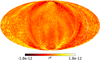 |
Fig. 1. Map level difference in temperature of the new SHT convolution algorithm compared to the old Conviqt approach, observed using the identical pointing of the first year of the 30 GHz Planck detectors. The differences are at the level of machine precision, indicating full agreement between the two algorithms. |
Figure 2 compares the runtime between the two approaches for a test configuration with an elliptical beam and a fixed sky model, and with mmax = 0 (using only the radially symmetric part of the beam) and mmax = 10, respectively. In both cases, the new implementation outperforms the old approach at all but the lowest values of lmax, where the data read time dominates. Additionally, for compatibility with the old libconviqt approach, this test was performed with an older version of libsharp, so we expect that the new algorithm scales even more favourably than this with the latest implementation. We note that this is a significant real-life advantage of the new approach: any improvement in SHT libraries, which typically are subject to intensive algorithm development and code maintenance, translates directly into a computational improvement for the convolution algorithm.
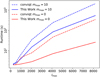 |
Fig. 2. Runtime comparison between the libconviqt approach and the new spin-SHT approach for the convolution of an elliptical Gaussian with a set of random sky al, ms. This work ties or outperforms the previous approach for all values of lmax from 256 to 8192 for both mmax values shown. We note the log scale on the y-axis. |
3. Sidelobe models
Figure 3 shows characteristic sidelobe response functions evaluated at a fixed frequency on the sky for a detector in each Planck LFI band. The sidelobe response for each detector within a single Planck band look visually quite similar, so only these representative ones are shown here. Each one is stored on disk as a set of alm’s with lmax = 512 and mmax = 100.
 |
Fig. 3. Maps of the sidelobe response on the sky from a representative detector at (left to right) 30 GHz, 44 GHz, and 70 GHz. The beam orientation is such that the main beam is pointed directly at the north pole in these maps. The intensities are normalized such that the main beams have unit power at l = 0. |
3.1. Main beam treatment
In the BEYONDPLANCK analysis, the sidelobe and main beam components of the sky response are separated, and the sidelobes are treated as a nuisance signal similar to the orbital dipole correction term, as can be seen in the BEYONDPLANCK global parametric model of the data:
![$$ \begin{aligned} \begin{aligned} d_{j,t}&= g_{j,t}\left[\mathsf P _{tp,j}\mathsf B _{pp^\prime ,j}\sum _{c} \mathsf M _{cj}(\beta _{p^\prime }, \Delta bp^{j})a^c_{p^\prime } + s^{\mathrm{orb} }_{j,t} + s^{\mathrm{fsl} }_{j,t}\right] \\&~\;+ s^{\mathrm{1hz} }_{j,t} + n^{\mathrm{corr} }_{j,t} + n^{\mathrm{w} }_{j,t}. \end{aligned} \end{aligned} $$](/articles/aa/full_html/2023/07/aa43138-22/aa43138-22-eq20.gif)
The other terms in this equation are discussed in detail in BeyondPlanck Collaboration (2023), but here the main beam signal is denoted as Bpp′, j and the sidelobe signal is extracted from the signal contribution and expressed as  . This distinction allows the sidelobes to be treated separately from the main beam in all respects. Treating the main beam using the Conviqt formalism of this paper would be possible, but the additional precision needed to model it accurately would require much higher values of lmax, and, therefore, greatly increased computational time and memory requirements.
In the BEYONDPLANCK analysis, the main beam is used (in conjunction with the sidelobes) to compute the full 4π dipole response, as detailed in Sect. 3.3. Additionally, a Gaussian main beam approximation is used during component separation to smooth the sky model to the appropriate beam resolution for each channel. During mapmaking, beam effects are ignored and the beam is assumed to be pointed at the center of each pixel.
3.2. Sidelobe normalization
We adopted a normalization of the sidelobes that differs slightly from the normalization used within the Planck LFI collaboration. The Planck 2018 LFI beam products leave a small portion (around 1%) of known missing power within the system unassigned due to uncertainties about to which component it should be assigned (Planck Collaboration IV 2016). In the current analysis, we adopted the same approximation as for Planck DR4 (Planck Collaboration Int. LVII 2020) and renormalized the beam transfer function such that this power would be distributed proportionally at each l; that is, we rescaled the beam transfer function Bl so that its full sky integral would be B0 = 1. This re-scaling is equivalent to assigning the unknown beam power uniformly over the entire beam. We note that this normalization is, in either case, always done before any higher-level analysis for both Planck 2018 and DR4; the only difference is whether the renormalization ought to be performed by external users through a deconvolution of a non-unity normalized main beam transfer function or not.
3.3. Orbital dipole and quadrupole sidelobe response
The treatment of the sidelobes is also important when generating orbital dipole and quadrupole estimates. Because Planck is calibrated primarily from the dipole measurements (Planck Collaboration I 2020; Planck Collaboration Int. LVII 2020; Gjerløw et al. 2023), the sidelobe’s contribution to the dipole can directly result in an absolute calibration error if not handled appropriately. While the CMB Solar dipole can easily be handled using the Conviqt approach described in Sect. 2.1, the orbital dipole is not sky-stationary and thus must be handled separately.
BEYONDPLANCK generates orbital dipole and quadrupole estimates directly from the Planck pointing information, using the satellite velocity data that has been stored at low resolution (one measurement per pointing period). With this information, it is possible to estimate the orbital dipole and quadrupole amplitude for each timestep, allowing the time-domain removal of the signal before it contaminates the final products with non-sky-stationary signal artifacts. Additionally, once this signal has been isolated from the raw data, it can be used as an aid in the calibration routines because of its highly predictable structure.
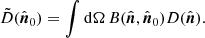
BEYONDPLANCK uses the same technique as Planck DR4 (see Appendix C of Planck Collaboration Int. LVII 2020) to generate the orbital dipole and quadrupole estimate. That is, we can express the signal  seen by a detector observing a fixed direction,
  , as the convolution of the dipole and quadrupole signal on the sky,
  , with the full 4π beam response,
  ,
,
Here it is useful to break the dipole signal up into three orthogonal components in the standard Cartesian coordinates (x, y, z) and we adopt the convention that the main beam points toward the north pole in our coordinate system.
The orbital CMB dipole and quadrupole can be expressed as a Doppler shift in each direction (Notari & Quartin 2015):
![$$ \begin{aligned} D(\hat{\boldsymbol{n}}) = T_0\left[ \beta \cdot \hat{\boldsymbol{n}}(1 + q\boldsymbol{\beta } \cdot \hat{\boldsymbol{n}}) \right], \end{aligned} $$](/articles/aa/full_html/2023/07/aa43138-22/aa43138-22-eq27.gif)
where β is the satellite velocity divided by the speed of light  ; T0 is the CMB temperature and q is the quadrupole factor dependent on the frequency ν, defined by
Inserting these expressions into Eq. (15), we obtain:
![$$ \begin{aligned} \begin{aligned} \tilde{D}&= T_0 \int \mathrm{d}\Omega _{\hat{\boldsymbol{n}}} B(\hat{\boldsymbol{n}}, \hat{\boldsymbol{n}}_0) \left[ x \ \beta _x + { y}\ \beta _{ y} + z\ \beta _z \right. \\&~\;+q\left(x^2\ \beta ^2_x + { y}^2\ \beta ^2_{ y} + z^2\ \beta ^2_z \right. \\&~\;+\left. \left. 2x{ y}\ \beta _x\beta _{ y} + 2xz\ \beta _x\beta _z + 2{ y}z\ \beta _{ y}\beta _z\right) \right], \end{aligned} \end{aligned} $$](/articles/aa/full_html/2023/07/aa43138-22/aa43138-22-eq30.gif)
where  is a unit direction vector that is also the integration variable and
  is the fixed direction of the satellite pointing for this timestep. We note that the geometric factors in this expression may be precomputed as
and, thus, we see that Eq. (17) may be written in the following form:
![$$ \begin{aligned} \tilde{D}&= T_0 \left[ S_x \ \beta _x + S_{ y}\ \beta _{ y} + S_z\ \beta _z \right. \nonumber \\&~\;+q\left(S_{xx}\ \beta ^2_x + S_{{ y}{ y}}\ \beta ^2_{ y} + S_{zz}\ \beta ^2_z \right. \nonumber \\&~\;+2S_{x{ y}} \left.\left.\beta _x\beta _{ y} + 2S_{xz}\ \beta _x\beta _z + 2S_{{ y}z}\ \beta _{ y}\beta _z\right) \right]. \end{aligned} $$](/articles/aa/full_html/2023/07/aa43138-22/aa43138-22-eq34.gif)
To compute  for an arbitrary beam orientation, we simply need to rotate the satellite pointing and velocity vectors into the coordinate system used to define S, and then we can evaluate Eq. (19) very quickly.
BEYONDPLANCK further accelerates this operation by computing this rotation for only one point in twenty (chosen so as to still fully sample the dipole) and using a spline to interpolate between them. This saves the cost of calculating a new rotation matrix at each step, and instead relies on the smoothness of the signal to ensure continuity. The algorithm treats the final few points of each pointing period that do not divide evenly into the subsampling factor separately. This allows for the use of regular bin widths, which greatly speeds up the splining routines, while the final few points are calculated using the slower rotation matrix technique.
4. Sidelobe estimates
4.1. Posterior mean corrections
Figure 4 shows the mean sidelobe signal estimates at each of the three LFI frequencies for the entire mission, co-added across each frequency and projected into sky coordinates, identically to the way the true sky signal is treated. Each map is averaged over 90 Gibbs samples produced in the main BEYONDPLANCK analysis (BeyondPlanck Collaboration 2023), after discarding burn-in and a thinning of the remaining chain by a factor of ten.
 |
Fig. 4. Maps of the sidelobes convolved with the sky at each of the three LFI frequencies. From top to bottom: 30 GHz, 44 GHz and 70 GHz. Left column: unpolarized sky signal, central column: Q polarization and right column: U. Note the difference in the colour scales required to see the same level of detail in all three channels. |
We note that these maps follow the traditional Planck LFI method of sidelobe correction by producing these signals in the time domain during TOD processing. These templates are therefore exactly correct for the maps produced by these pipeline runs, but will not precisely match up with analyses that use different data cuts, flagging or channel selection.
These results appear visually similar to the corresponding Planck DPC results presented in Fig. 7 of Planck Collaboration III (2016). The main difference is that the current results also include the CMB dipole, whereas the LFI 2015 DPC analysis showed the sidelobe pickup of dipole-subtracted maps. We see that the sidelobe signal is strongest at 30 GHz and that the dominant features in the co-added sky maps consist of a series of rings created by the interplay between the sidelobe pickup and bright Galactic plane features.
Figure 4 also clearly indicates that the overall level of sidelobe pickup at 44 GHz is significantly lower than for the 30 and 70 GHz channels. This is due to the particular location in the focal plane of two of the three 44 GHz feedhorns, which results in a significant under-illumination of both the primary and secondary reflectors of the Planck telescope for those two horns (see Fig. 4 of Sandri et al. 2010).
4.2. Error propagation
In addition to the posterior mean sidelobe maps, the BEYONDPLANCK pipeline outputs also provide an estimate of the sidelobe stability and statistical variation. Figure 5 shows the rms maps generated from the same sample of sidelobe signal estimates used in Fig. 4. Clear evidence of the scanning pattern can be seen, as expected. The sharp vertical lines visible in polarization (clearest in 30 GHz Q and U at the top, and 44 GHz U at the top and bottom) have been previously examined by the Planck team and they are caused by a chance alignment between the non-dense Planck scanning strategy and the shape of the HEALPix pixels. For an example of this effect, see Fig. 15 of Planck Collaboration VII (2014).
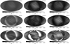 |
Fig. 5. Sidelobe rms maps at each of the three LFI frequencies. From top to bottom: 30 GHz, 44 GHz, and 70 GHz. Left column: unpolarized sky signal, central column: Q polarization and right column: U. Again note the different colour scales. |
These posterior rms maps cannot be considered true sidelobe error estimates, however, since they do not account for uncertainties in the sidelobe response itself. Rather, they only show the change in the estimated sidelobe signal due to sky model variations from component separation. Full sidelobe error propagation would require sampling over the physical parameters that determine the detectors’ sidelobe response on the sky. Sampling the full set of optical model parameters is likely to be infeasible due to excessive computational time, however, identifying a minimal parameter set that may account for the main potential variations in the sidelobe response functions, as well as precomputing response functions over a grid of such parameters, would result in physically motivated uncertainties for the sidelobe models. This approach will be developed for future applications such as the LiteBIRD mission (Hazumi et al. 2019).
5. Impact on frequency and component maps
To assess the importance of sidelobe corrections on frequency and component maps, we performed two runs of the Commander code, starting from the same input data as the main pipeline run and with the identical random seed 12345678. As a comparison, we removed the far sidelobe correction from one of these secondary pipeline executions, and we differentiated the results between these two pipelines. The random seed is required by the sampling approach of the BEYONDPLANCK pipeline to explore the posterior distribution of many of the sampled parameters; identical seeds will result in identical samples barring other differences.
Figure 6 shows the differences in the frequency maps between the two cases in temperature, where the effects are the most obvious. The only large-scale features that can clearly be seen are the small dipole differences (most clearly visible at 70 GHz). These are directly caused by the dipolar component seen in Fig. 4, since this contribution to the total sky signal that was in the sidelobe term is now unaccounted for. In previous analyses, these dipole contributions were handled through specific modeling of exactly these effects, but this test makes it explicitly clear that correct dipole measurements require accurate knowledge of the sidelobe pickup.
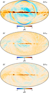 |
Fig. 6. Frequency map difference plots smoothed to one degree at (top to bottom) 30, 44, and 70 GHz, comparing two pipeline executions with the same seed, one of which has no sidelobe correction. |
Next, we see two more features in the difference maps that are more localized. The first of these are the ring structures that match the actual sidelobe map structures quite closely, which are, of course, the same rings from Fig. 4, and are not accounted for in the second pipeline run without sidelobe corrections. Additionally, there are some uniform residuals that are visible in the Galactic plane regions of the difference maps. These are caused by a calibration mismatch between the detectors at a single frequency. Since each of the detectors now sees a slightly different dipole signal on the sky, depending on its specific sidelobe response, their calibrations do not agree with one another, which causes signal residuals that are most visible in the plane where the signal amplitude is highest.
Figure 7 shows the differences in component maps from this same comparison, again in temperature. The CMB as well as the three low-frequency foreground components are estimated using the standard Commander3 technique described in Andersen et al. (2023). The AME component sees similar issues to the ones seen by the frequency maps above: the dipole is slightly incorrect, there are sidelobe-esque stripes, and the Galactic plane shows a strong residual. All of these effects have been seen directly in the frequency maps. The dipole difference seen here is precisely the one that contributes to the difference in calibration between the two different pipeline executions.
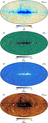 |
Fig. 7. Component map difference plots for (top to bottom) CMB, synchrotron, AME and freefree emission, comparing two pipeline executions with the same seed, one of which has no sidelobe correction. |
The other three components (synchrotron, CMB, and free-free) show relatively fewer structural differences. They have absorbed some of the sidelobe-like ring structures, but the primary difference can be seen most clearly in the Galactic plane. Here, we notice a large residual caused by the inaccurate model of the Galactic emission being altered slightly by the gain and calibration differences between the two runs. As the Galactic emission is significantly brighter than the rest of the sky, small changes in calibration produce large errors such as the ones seen here.
Finally, in Fig. 8, we show the correlated noise map difference at 30 GHz between the two runs. We see that some of the missing sidelobe signal has been accommodated by the correlated noise component. These structures mirror the strongest sidelobe-like signals in the 30 GHz difference map in the top panel of Fig. 6. The fact that ncorr can accommodate some sidelobe residuals is, in fact, helpful, as it allows for some leeway in the final sidelobe model, in the sense that small uncertainties and artifacts that are inconsistent between different frequency channels will be mostly absorbed into the correlated noise component, rather than in the sky maps. The differences that we see in the maps, however, indicate that this process is not perfect, as some of the spurious signal still makes it to the final maps without a perfect sidelobe model. For a real-world example of these issues, we refer the interested reader to the ongoing BEYONDPLANCK re-analysis of the WMAP data, for which far sidelobe contamination appears to be a dominant problem (Watts et al. 2023).
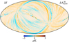 |
Fig. 8. Difference in correlated noise, projected into the map domain at 30 GHz comparing two pipeline executions with the same seed, one of which has no sidelobe correction. |
The residual errors seen in Figs. 6 and 7 are also present in the BEYONDPLANCK analysis, albeit at much lower levels. We know that our knowledge and modelling of the sidelobes are imperfect, as they are based on limited measurements of the physical LFI sidelobes and some of the power is unaccounted for. Future applications that aim for a robust measurement of primordial B-modes (constraining the tensor-to-scalar ratio r ≤ 0.01), will be required to marginalize over the sidelobe uncertainties in some manner, either directly via a Gibbs sampling of a subset of the instrument parameters or by parameterizing and fitting sidelobe error estimates. We do not believe that the sidelobe contribution causes significant errors in the LFI sample sets produced by BEYONDPLANCK, as it is unlikely to be more than a 10% error on the sidelobe estimates of Fig. 4. At 30 GHz, this corresponds to at most a 0.05% error in our temperature maps and a 1% error in polarization. We do expect, however, that as instrumental sensitivities improve, especially in polarization, this sidelobe term will need to be modeled very accurately, and the corresponding uncertainties must be propagated properly, for instance, using methods similar to those presented in this paper.
6. Summary and conclusions
This paper presents a formulation of the Conviqt algorithm in terms of spin-weighted spherical harmonics. This algorithm has already been already implemented in the latest versions of the libconviqt library and it has now also been re-implemented directly into Commander, where it is used for sidelobe corrections for the BEYONDPLANCK analysis framework. Based on the Monte Carlo samples produced in that analysis, we have presented novel posterior mean and standard deviation maps for each of the three Planck LFI frequency bands.
The full-sky sidelobe treatment techniques presented here are easily generalizable to other experiments, and can be tuned to match the required spatial characteristics of other instruments simply by adjusting the spherical harmonic bandpass parameters, lmax and mmax, of the sidelobe description. The only requirement for using the code with a new instrument is a HEALPix-compatible description of the sidelobe response function per detector. The more accurate this characterization of the instrument is, the closer the sidelobe estimation will get to approximating the true sidelobe contamination in the timestream.
We note that the approach presented here is less useful for ground- or balloon-based experiments where the dominant sidelobe pickup contains radiation from an environmental source. This pickup is not sky-synchronous, and, thus, it cannot be modeled purely as a beam-sky convolution, but instead must include additional contributions from, for example, telescope baffles, ground pickup, or clouds. For these types of experiments, other techniques such as aggressive baffling are likely to be better suited.
We also stress that the current implementation only supports sidelobe error propagation for sky model uncertainties – and not the uncertainties in the actual sidelobe response function itself, which are very likely to dominate the total sidelobe error budget. Future works should therefore aim to introduce parametric models for the sidelobe response itself, and sample (or at least marginalize) over the corresponding free parameters, as these are typically among the most important unknowns for many experiments.
Finally, we note that future CMB experiments such as LiteBIRD, targeting low B-mode limits, may need to consider more complex ways of handling sidelobes and beams. The ultimate solution in this respect is 4π beam convolution for every single timestep, which could be achieved using a similar framework to the approach discussed here. This would remove the sidelobes as a nuisance signal from the data model of Eq. (13) and instead incorporate them directly into the beam term, Bpp′, j. This approach should be feasible for a relatively low-resolution experiment such as LiteBIRD and will be further investigated in a subsequent study.
In this paper, ϑ and φ are the co-latitude and longitude of a location on the sphere, i.e., they have the same meaning as in the HEALPix context (Górski et al. 2005).
Acknowledgments
We thank Prof. Pedro Ferreira and Dr. Charles Lawrence for useful suggestions, comments and discussions. We also thank the entire Planck and WMAP teams for invaluable support and discussions, and for their dedicated efforts through several decades without which this work would not be possible. The current work has received funding from the European Union’s Horizon 2020 research and innovation programme under grant agreement numbers 776282 (COMPET-4; BEYONDPLANCK), 772253 (ERC; BITS2COSMOLOGY), and 819478 (ERC; COSMOGLOBE). In addition, the collaboration acknowledges support from ESA; ASI and INAF (Italy); NASA and DoE (USA); Tekes, Academy of Finland (grant no. 295113), CSC, and Magnus Ehrnrooth foundation (Finland); RCN (Norway; grant nos. 263011, 274990); and PRACE (EU).
References
- Andersen, K. J., Aurlien, R., Banerji, R., et al. 2023, A&A, 675, A13 (BeyondPlanck SI) [NASA ADS] [CrossRef] [EDP Sciences] [Google Scholar]
- Barnes, C., Hill, R. S., Hinshaw, G., et al. 2003, ApJS, 148, 51 [NASA ADS] [CrossRef] [Google Scholar]
- BeyondPlanck Collaboration (Andersen, K. J., et al.) 2023, A&A, 675, A1 (BeyondPlanck SI) [Google Scholar]
- Burigana, C., Maino, D., Górski, K. M., et al. 2001, A&A, 373, 345 [NASA ADS] [CrossRef] [EDP Sciences] [Google Scholar]
- Gjerløw, E., Ihle, H. T., Galeotta, S., et al. 2023, A&A, 675, A7 (BeyondPlanck SI) [NASA ADS] [CrossRef] [EDP Sciences] [Google Scholar]
- Goldberg, J. N., Macfarlane, A. J., Newman, E. T., Rohrlich, F., & Sudarshan, E. C. G. 1967, J. Math. Phys., 8, 2155 [NASA ADS] [CrossRef] [Google Scholar]
- Górski, K. M., Hivon, E., Banday, A. J., et al. 2005, ApJ, 622, 759 [Google Scholar]
- Hazumi, M., Ade, P., Akiba, Y., et al. 2019, J. Low Temperature Phys., 194, 443 [NASA ADS] [CrossRef] [Google Scholar]
- Lewis, A. 2005, Phys. Rev. D, 71, 083008 [Google Scholar]
- Notari, A., & Quartin, M. 2015, J. Cosmol. Astropart. Phys., 2015, 047 [CrossRef] [Google Scholar]
- Planck Collaboration III. 2014, A&A, 571, A3 [NASA ADS] [CrossRef] [EDP Sciences] [Google Scholar]
- Planck Collaboration VII. 2014, A&A, 571, A7 [NASA ADS] [CrossRef] [EDP Sciences] [Google Scholar]
- Planck Collaboration III. 2016, A&A, 594, A3 [NASA ADS] [CrossRef] [EDP Sciences] [Google Scholar]
- Planck Collaboration IV. 2016, A&A, 594, A4 [NASA ADS] [CrossRef] [EDP Sciences] [Google Scholar]
- Planck Collaboration XII. 2016, A&A, 594, A12 [NASA ADS] [CrossRef] [EDP Sciences] [Google Scholar]
- Planck Collaboration I. 2020, A&A, 641, A1 [NASA ADS] [CrossRef] [EDP Sciences] [Google Scholar]
- Planck Collaboration Int. XLVI. 2016, A&A, 596, A107 [NASA ADS] [CrossRef] [EDP Sciences] [Google Scholar]
- Planck Collaboration Int. LVII. 2020, A&A, 643, A42 [NASA ADS] [CrossRef] [EDP Sciences] [Google Scholar]
- Prézeau, G., & Reinecke, M. 2010, ApJS, 190, 267 [CrossRef] [Google Scholar]
- Reinecke, M., & Seljebotn, D. S. 2013, A&A, 554, A112 [NASA ADS] [CrossRef] [EDP Sciences] [Google Scholar]
- Sandri, M., Villa, F., Bersanelli, M., et al. 2010, A&A, 520, A7 [NASA ADS] [CrossRef] [EDP Sciences] [Google Scholar]
- Svalheim, T. L., Andersen, K. J., Aurlien, R., et al. 2023, A&A, 675, A14 (BeyondPlanck SI) [NASA ADS] [CrossRef] [EDP Sciences] [Google Scholar]
- Toral, M., Ratliff, R., Lecha, M., et al. 1989, Antennas and Propagation, IEEE Transactions on AP-37, 171 [CrossRef] [Google Scholar]
- Wandelt, B. D., & Górski, K. M. 2001, Phys. Rev. D, 63, 123002 [NASA ADS] [CrossRef] [Google Scholar]
- Watts, D. J., Galloway, M., Ihle, H. T., et al. 2023, A&A, 675, A16 (BeyondPlanck SI) [NASA ADS] [CrossRef] [EDP Sciences] [Google Scholar]
- Wu, J. H. P., Balbi, A., Borrill, J., et al. 2001, ApJS, 132, 1 [NASA ADS] [CrossRef] [Google Scholar]
All Figures
|
Fig. 1. Map level difference in temperature of the new SHT convolution algorithm compared to the old Conviqt approach, observed using the identical pointing of the first year of the 30 GHz Planck detectors. The differences are at the level of machine precision, indicating full agreement between the two algorithms. |
| In the text | |
|
Fig. 2. Runtime comparison between the libconviqt approach and the new spin-SHT approach for the convolution of an elliptical Gaussian with a set of random sky al, ms. This work ties or outperforms the previous approach for all values of lmax from 256 to 8192 for both mmax values shown. We note the log scale on the y-axis. |
| In the text | |
|
Fig. 3. Maps of the sidelobe response on the sky from a representative detector at (left to right) 30 GHz, 44 GHz, and 70 GHz. The beam orientation is such that the main beam is pointed directly at the north pole in these maps. The intensities are normalized such that the main beams have unit power at l = 0. |
| In the text | |
|
Fig. 4. Maps of the sidelobes convolved with the sky at each of the three LFI frequencies. From top to bottom: 30 GHz, 44 GHz and 70 GHz. Left column: unpolarized sky signal, central column: Q polarization and right column: U. Note the difference in the colour scales required to see the same level of detail in all three channels. |
| In the text | |
|
Fig. 5. Sidelobe rms maps at each of the three LFI frequencies. From top to bottom: 30 GHz, 44 GHz, and 70 GHz. Left column: unpolarized sky signal, central column: Q polarization and right column: U. Again note the different colour scales. |
| In the text | |
|
Fig. 6. Frequency map difference plots smoothed to one degree at (top to bottom) 30, 44, and 70 GHz, comparing two pipeline executions with the same seed, one of which has no sidelobe correction. |
| In the text | |
|
Fig. 7. Component map difference plots for (top to bottom) CMB, synchrotron, AME and freefree emission, comparing two pipeline executions with the same seed, one of which has no sidelobe correction. |
| In the text | |
|
Fig. 8. Difference in correlated noise, projected into the map domain at 30 GHz comparing two pipeline executions with the same seed, one of which has no sidelobe correction. |
| In the text | |
Current usage metrics show cumulative count of Article Views (full-text article views including HTML views, PDF and ePub downloads, according to the available data) and Abstracts Views on Vision4Press platform.
Data correspond to usage on the plateform after 2015. The current usage metrics is available 48-96 hours after online publication and is updated daily on week days.
Initial download of the metrics may take a while.