| Issue |
A&A
Volume 675, July 2023
|
|
|---|---|---|
| Article Number | A161 | |
| Number of page(s) | 15 | |
| Section | Numerical methods and codes | |
| DOI | https://doi.org/10.1051/0004-6361/201936851 | |
| Published online | 14 July 2023 | |
A group finder algorithm optimised for the study of local galaxy environments
Sub-department of Astrophysics, Department of Physics, University of Oxford, Denys Wilkinson Building, Keble Road, Oxford OX1 3RH, UK
e-mail: mark.graham@physics.ox.ac.uk
Received:
6
October
2019
Accepted:
2
October
2020
Context. The majority of galaxy group catalogues available in the literature use the popular friends-of-friends algorithm which links galaxies using a linking length. One potential drawback to this approach is that clusters of points can be linked with thin bridges which may not be desirable. In order to study galaxy groups, it is important to obtain realistic group structures.
Aim. Here we present a new simple group finder algorithm, TD-ENCLOSER, that finds the group that encloses a target galaxy of interest.
Methods. TD-ENCLOSER is based on the kernel density estimation method which treats each galaxy, represented by a zero-dimensional particle, as a two-dimensional circular Gaussian. The algorithm assigns galaxies to peaks in the density field in order of density in descending order (‘top down’) so that galaxy groups ‘grow’ around the density peaks. Outliers in under-dense regions are prevented from joining groups by a specified hard threshold, while outliers at the group edges are clipped below a soft (blurred) interior density level.
Results. The group assignments are largely insensitive to all free parameter variations apart from the hard density threshold and the kernel standard deviation, although this is a known feature of density-based group finder algorithms and it operates with a computing speed that increases linearly with the size of the input sample. In preparation for a companion paper, we also present a simple algorithm to select unique representative groups when duplicates occur.
Conclusions. TD-ENCLOSER is tested on a mock galaxy catalogue using a smoothing scale of 0.3 Mpc and is found to be able to recover the input group distribution with sufficient accuracy to be applied to observed galaxy distributions.
Key words: galaxies: clusters: general / galaxies: groups: general / methods: numerical
© ESO 2023
1. Introduction
It has been known since the first large-scale galaxy surveys that galaxies are not randomly distributed throughout the Universe, but they are preferentially found in groups and clusters. This structure traces the underlying dark matter distribution which cannot be observed directly. Moreover, many galaxy properties depend on the local environment, including the morphology and colour (Blanton et al. 2005; Blanton & Moustakas 2009). Therefore, it is of great interest to produce accurate and reliable group catalogues of nearby galaxies with which to study the properties of galaxies as a function of the environment. Only with the advent of large spectroscopic surveys has it been possible to obtain accurate positions of galaxies using spectroscopic redshifts, which provide a much greater accuracy than photometric redshifts. While the first spectroscopic galaxy survey (CfA1 Redshift Survey; Huchra & Geller 1982; Geller & Huchra 1983) only used a single slit to obtain the redshift, more recent surveys have used multi-slit or fibre-optic spectrographs to observe hundreds of thousands of galaxies with spectroscopy. Notable examples are the Two Degree Field Galaxy Redshift Survey (2dFGRS; Colless et al. 2001), the Galaxy And Mass Assembly survey (GAMA; Driver et al. 2009, 2011), and the Sloan Digital Sky Survey (see York et al. 2000 for a technical summary, Gunn et al. 2006 for a summary of the SDSS telescope, Smee et al. 2013 for a description of the spectrographs, and Blanton et al. 2017 for a summary of SDSS-IV). Collectively, these surveys have provided the basis for studying galaxy environments across huge samples.
The availability of such large datasets allows the opportunity to produce galaxy group catalogues. Many catalogues have been produced by various research teams using data from one or more of these surveys. Although some catalogues have been based purely on data from the 2dFGRS (Merchán & Zandivarez 2002; Eke et al. 2004; Yang et al. 2005) or the GAMA survey (G3Cv7, Robotham et al. 2011), the most productive survey for group catalogues has been the SDSS. Most significant data releases have been complemented by a group catalogue based on the spectroscopic sample, including DR2 (Miller et al. 2005), DR3 (Merchán & Zandivarez 2005), DR4 (Yang et al. 2007, updated to DR7), DR5 (Tago et al. 2008), DR7 (Tago et al. 2010; Muñoz-Cuartas & Müller 2012), DR8 (Tempel et al. 2012), DR10, (Tempel et al. 2014) and DR12 (Tempel et al. 2017). There are many other catalogues available that are based on surveys, including for example the 6dFGS Galaxy Survey Final Redshift Release Catalogue (zmedian = 0.053; Jones et al. 2009) and the 2MASS Redshift Survey (2MRS) Catalogue (z90th = 0.05; Huchra et al. 2012)1.
The power of these catalogues lies in their scope for studying galaxy properties across large samples to obtain powerful statistical results. However, they are almost always based on the friends-of-friends (FoF) method to assign galaxies to groups (Huchra & Geller 1982; Davis et al. 1985). This simple method uses a linking metric to assign particles to halos and, as such, is a frequent choice for assigning galaxies to halos in dark matter simulations (Eke et al. 2004; Tempel et al. 2016; see Knebe et al. 2013 for a review). The linking metric is usually defined to be a constant fraction of the mean particle separation. For magnitude-limited surveys, such as the SDSS spectroscopic survey, the linking length varies with z to account for the change in the luminosity function with z (Huchra & Geller 1982). One potential issue with the FoF method is that groups can end up being joined by thin bridges, which may not be desirable (or even harmful). Yang et al. (2005) combined the FoF method with an iterative procedure that first estimates the location, mass, and radius of dark matter halos based on the galaxy distribution, before assigning galaxies to those halos and recomputing the halos. Miller et al. (2005) used a spherical aperture and information about the galaxy colours to identify clusters based on the probability of obtaining the observed galaxy distribution randomly.
Another independent method for estimating the underlying probability density function of some discrete data is the kernel-density estimation (KDE) method (Parzen 1962). The premise behind this approach is that by replacing particles, representing galaxies, of zero size by kernels of non-zero size, a continuous probability density function can be obtained across the coordinate space. To find clumps or groups in the particle distribution, all one needs to do is locate local maxima in the density function. There are a number of algorithms which assign particles to groups based on the density field, although the details of the method can vary somewhat between them. However, there are no group catalogues currently available that are based on redshift surveys and use the KDE method. See Knebe et al. (2013) for a complete review of group-finder algorithms used in galaxy simulations.
Our ultimate goal is to study the environment of galaxies in the SDSS-IV Mapping Nearby Galaxies at Apache Point Observatory (MaNGA) survey (Bundy et al. 2015) in as much detail as possible. To this end, we have paid great attention to obtaining an accurate catalogue of galaxies and galaxy groups. A key advantage of the sample of galaxies observed by the MaNGA survey is that it is small enough that the neighbours of MaNGA galaxies can be assessed visually. We take the opportunity to develop an algorithm that assigns galaxies to groups based on the underlying galaxy distribution, with the intention of identifying groups that match what one might conclude from looking at the galaxy distribution by eye.
This paper is split as follows. We first discuss previous group finder algorithms that use the KDE method (Sect. 2.1) before introducing our top-down approach to KDE-based clustering (Sect. 2.2). In Sect. 2.3, we briefly describe the MaNGA survey (Bundy et al. 2015) which provides the first use case for our new group-finder algorithm, TD-ENCLOSER2, presented in Sect. 3, which adapts features of previous algorithms and is suitable for sample sizes of up to ∼105 particles. We focus on providing a simple routine that provides a careful treatment of small groups and cropping outliers from large groups. We use the ‘hill-climbing’ method but only consider directions where a galaxy is known to exist. We also adapt parameters from the HOP method of Eisenstein & Hut (1998, hereafter EH98). We then test our algorithm on a mock galaxy catalogue to demonstrate its operation and effectiveness (Sect. 4).
In Graham et al. (2019a, Paper II), we use TD-ENCLOSER to find the nearest neighbours to MaNGA galaxies. The set of neighbours that we find depends on the MaNGA galaxy, and if MaNGA galaxies are local to each other, then the same intrinsic groups may be found multiple times but with slight differences between each set. Ultimately we want to construct a group catalogue for MaNGA galaxies where each MaNGA galaxy lives in a well-defined environment. This requires us to select unique environments for each MaNGA galaxy, which we achieve in Sect. 5. In Graham et al. (2019b, Paper III), we use this catalogue to conduct a large study of galaxy angular momentum and environment, with a few specific examples shown in Graham et al. (2019c, Paper IV).
Throughout this work, we adopt standard values for the cosmological parameters, close to the latest measured values (Planck Collaboration XIII 2016). We take the value of the Hubble constant, H0, to be 70 km s−1 Mpc−1 and assume a flat cosmology where ΩM, Ωk and ΩΛ are 0.3, 0 and 0.7 respectively.
2. KDE-based clustering
2.1. Previous KDE-based group finder algorithms
There are many algorithms present in the literature that use a kernel density estimator to group particles into clusters. Many of these were optimised for N-body dark matter simulations and hence deal with 𝒪(106) particles. The first to be developed was DENMAX (Bertschinger & Gelb 1991; Gelb & Bertschinger 1994) which uses an interpolation of the particle distribution to define a regular rectangular grid. Particles slide from their original locations towards a nearby dense grid cell with a force that is proportional to the local gradient, so that the particles follow a fluid equation. All particles that settle at the same peak are considered to be part of the same halo. Particles at the edges are clipped using an energy constraint evaluated by comparing a particle’s kinetic and potential energy at different timestamps. Spline Kernel Interpolative Denmax (SKID; Weinberg et al. 1997) is an updated version of DENMAX that employs a spline kernel interpolation with a variable kernel size, rather than a regular grid of uniform kernel size. The densities are only measured at the particle locations with particles moving in the same way as DENMAX towards density peaks. The HOP method (EH98) is inspired by SKID in that densities are only calculated at particle locations. However, instead of particles following the density field via a fluid equation, particles ‘hop’ to the densest neighbour within the nearest Nhop neighbours. Particles hop until they reach the densest particle and all particles that hop to the same particle are assigned to the same halo. A set of six parameters, not including the kernel bandwidth, are used to merge groups and clip outliers.
DENCLUE (Hinneburg & Keim 1998; Hinneburg & Gabriel 2007) is another KDE-based group finder algorithm. From a given particle, the algorithm climbs hills defined by the density field and assigns all particles that climb to the same hill to the same cluster. This method has the advantage of many density-based methods in that there is a unique result regardless of the order in which particles are considered. DENCLUE 2.0 (Hinneburg & Gabriel 2007) includes a variable step size to reduce the number of iterations by considering the local gradients, without compromising on accuracy. It also has a noise threshold which is used to discount local maxima which fail to reach this threshold. However, the algorithm does not set a minimum threshold for particles to be considered as members of a cluster and so a cluster can have members with density ≈0.
If limitations due to computing power or sample size were not an issue, then the precise and formal way to find groups would be to start from a particular galaxy and find the direction of maximal gradient in the density field. After moving a certain step size in that direction, the search would be repeated until the galaxy reaches a point where all gradients are negative. A helpful picture to have in mind is if the field were overturned so that peaks became valleys, then the galaxy would roll down in the direction of the steepest downwards slope, similar to a rain drop, before stopping at the bottom of the valley where all gradients are positive. We note that a similar method already exists and is known as ‘mean-shifting’ or ‘mode-seeking’ (for example Cheng 1995; see Carreira-Perpiñán 2015 for a review). In this method, a kernel is placed over a point and is shifted towards the direction where the density, set by the number of points, increases within the kernel defined by the mean-shift vector. While the ‘rain drop’ method would be the most rigorous solution to this problem, there are two drawbacks to implementing it computationally.
Firstly, the step size should be sensitive to the gradient so that a steeper gradient encourages a larger step size as in Hinneburg & Gabriel (2007). This can be fairly straightforward to implement based on the equations of motion in a potential for example. However, this will be inefficient for points which are far away from the peak or valley as the gradient will be small. The second obstacle is optimising the search for the direction of steepest gradient. Once the particle has initially found this direction, the search can be limited to ϕ ± Δϕ, where ϕ is the current direction of the steepest gradient and Δϕ is the field of view or equivalently the width of an arc. While this works in principle, the path to the top of the peak, or bottom of the valley, has the potential to be much longer than the distance travelled as the crow flies, especially if the topology is complex.
One option to simplify this is to roll down from peaks in the density and tag all particles that are met along the way. Here, the search stops at the foot of the hill where all gradients are positive. This approach requires prior knowledge of the location of the peaks but can, in theory, be more efficient than the method described above. Instead of moving from multiple points to a single location, this method moves outwards from a single location assigning particles to the peak along the way. This ‘hill-down’ approach was first applied in HD-DENCLUE by Xie et al. (2007) with the intention of finding groups of connected points in medical imaging data (see also Xie et al. 2010). In their approach, the data are finely gridded and all points on the grid are added to the cluster with each successive step down the hill. The edge or foot of the cluster is defined where the absolute value of the gradient falls below a predefined noise threshold. While this method works well for millions of particles (as is the case for imaging data), it becomes inefficient for smaller samples of a few hundred particles because all directions need to be searched from the point of view of the peak.
A similar approach was taken by Springel et al. (2001) who combined the FoF method with a ‘top-down’ method that can identify the background density field and substructure in a dark matter simulation. Their algorithm, called SUBFIND, sorts particles by their density and then ‘rebuilds’ the particle distribution by adding them to halos in order of decreasing density. Particles are only assigned to one subhalo so that they do not contribute to the mass of the parent halo, but Springel et al. (2001) find that this does not affect the parent halo a great deal as the substructure is usually at a scale that is small compared to the parent halo.
2.2. A top-down approach to KDE-based clustering
All of these algorithms have been optimised for millions of particles and hence are appropriate for producing group catalogues based on the dark matter distribution. However, we are interested in simply grouping galaxies together and obtaining directly observable relations and are not concerned with the dark matter distribution. As we are only focussing on the neighbours local to a specific sample of galaxies, that is the MaNGA galaxies, we do not need to consider large numbers of galaxies. Moreover, we would like to be able to detect all group sizes from two upwards. We would also like to be able to differentiate nearby peaks rather than merge them, which can happen with the HOP method for example (see Fig. 1 of EH98).
Our approach is to combine a ‘top-down’ method with a hill climbing method so that it is efficient for sample sizes of a few hundred to a few thousand particles. To keep our algorithm as simple as possible, we only consider straight lines between points while ignoring the surface topology. By considering galaxies in order of their density from highest to lowest, we identify the peaks before attracting galaxies towards those peaks. Hence, rather than sliding or hopping from a particular galaxy, we take a ‘top-down’ approach where we move out from regions of high density to regions of low density.
2.3. The MaNGA survey
Before describing TD-ENCLOSER in detail, we briefly summarise the MaNGA survey (Bundy et al. 2015) which provides the first use case for TD-ENCLOSER. MaNGA is an ambitious project designed to observe at least 10 000 galaxies with integral field spectroscopy over a six-year period. MaNGA is based at the dedicated SDSS telescope (Gunn et al. 2006; see Fukugita et al. 1996; Gunn et al. 1998 and Doi et al. 2010 for details about the photometry and camera) and is currently operating as part of SDSS-IV (Blanton et al. 2017). MaNGA uses the BOSS spectrographs which provide a spectral resolution R ∼ 2000 across the visible wavelength range (Smee et al. 2013). The survey employs a suite of 17 state-of-the-art integral field units (IFUs) ranging between 12″ and 32″ in diameter and each containing between 19 and 127 individual fibres each of which are 2″ in diameter (Drory et al. 2015; Law et al. 2015). The IFUs are plugged into plates which have been drilled with holes each corresponding to one of the 17 galaxies which are to be observed in the field of view. To fill in the gaps between fibres, a dithering scheme is used where the observations are repeated after each plate is moved by a distance slightly smaller than the fibre diameter in a triangular pattern so that three exposures are taken in total. For further details, see Yan et al. (2016a) about the survey design, execution, and initial data quality and Yan et al. (2016b) about the calibration technique for MaNGA.
Galaxies are sampled between z = 0.01 and z = 0.15 with a peak at about z = 0.03. A key feature of the selection criteria is that the sample has a flat distribution in stellar mass (Wake et al. 2017). The most luminous massive galaxies are observed at the higher redshifts within the range so that a minimum spatial resolution in terms of effective radius (Re) can be maintained. MaNGA is split into Primary, Secondary and Coloured enhanced samples (Wake et al. 2017). The observing targets for the primary and secondary samples require that 80% of the galaxies are observed with IFUs out to 1.5 and 2.5 Re respectively, with a minimum of 5 radial bins in both cases. As a result, the secondary sample is observed at a lower spatial resolution than the primary sample. The colour-enhanced sample is included to fill in the gaps in the colour distribution at fixed stellar mass and comprises of green valley galaxies as well as low mass red galaxies and high mass blue galaxies.
The raw data is reduced by the Data Reduction Pipeline (DRP; Law et al. 2016) and a suite of derived data products are produced by the Data Analysis Pipeline (DAP; see Westfall et al. 2019 for an overview and Belfiore et al. 2019 for details about continuum subtraction and emission line modelling). Both the reduced data and derived data products have been publicly released as part of DR15 (Aguado et al. 2019). A tool called ‘Marvin’ was released as part of DR15 that provides access to MaNGA data via a web App, a Python package of tools, and an API (Cherinka et al. 2019).
3. Description of TD-ENCLOSER
3.1. Definition of algorithm parameters
The algorithm we present here is similar to SUBFIND in that it considers galaxies by their density in decreasing order, but its function is an adaptation of the HOP method of EH98. EH98 solved two key problems regarding the separation of halos from their surroundings as well as the merging of groups by introducing six tunable parameters. Despite the added complexity, they showed that the result was insensitive to all but one of those parameters. We adopt four of these parameters and adapt three of them to our specific requirements. Another similarity between our algorithm and the one of EH98 is that we make three passes of the data, although the manner in which our passes operate differ.
Here we give details of the parameters that we adopt from EH98. They used δ to denote density but we use ρ instead as δ can also represent a difference. Firstly, we define ρouter as the minimum density required for a galaxy to be considered as part of a group. By setting this parameter, EH98 prevent particles in underdense regions from joining groups. We retain this functionality of ρouter in this work. This is the only parameter found by EH98 to have a significant impact on the final group distribution. Next, we define ρsaddle as a second contour level which, if ρsaddle ≠ ρouter, can be used to separate two peaks which are joined by a bridge where ρ ≥ ρouter (for example separating A and B from C in Fig. 1 of EH98). It could also be used to join two peaks which are separated by a local minimum where ρ ≥ ρsaddle (for example A and B in Fig. 1 of EH98). We use ρsaddle to exclude outliers from groups based on the density of one of their local neighbours.
Next, we adopt Nmerge. In EH98, this parameter is used to merge two nearby groups. If a particle and one of its nearest Nmerge neighbours are in different groups, then a boundary pair is defined between the particle and the densest of the Nmerge nearest neighbours. If the density of the boundary pair, defined to be the mean of the density of the two particles, is greater or equal to ρsaddle, then the two groups are merged. We use Nmerge and ρsaddle in a similar way to eject galaxies which lie far enough below ρsaddle. Specifically, we eject galaxies if the mean between their density and the maximum density of their Nmerge − 1 neighbours is less than ρsaddle. Hence, this decision is determined by the local galaxy distribution and ρsaddle is effectively a blurred boundary (see Sect. 3.2.5).
Finally, we adopt ρpeak. In EH98, if the density ρ of a peak is such that ρouter ≤ ρ < ρpeak, then the peak is only considered as part of a subgroup and is attached to a larger group with ρ > ρpeak. Here, we would like to detect small groups which may not have the density required to reach ρpeak. However, we do use ρpeak to decide whether to disconnect outliers from groups using ρsaddle and Nmerge. The final parameter is the kernel size σker although this parameter is general to all KDE-based methods and is not specific to EH98.
3.2. Algorithm methodology
In what follows, we explain the methodology behind TD-ENCLOSER, referring to the pseudocode given in Algorithm 1 by line number (for example line 1) and the one-dimensional visualisation shown in Fig. 1. In Algorithm 1, we only give the minimum amount of information required to implement the algorithm, leaving finer details to the text. To allow the reader to follow the decision making process, we have provided in Table 1 values for position along the x-axis and ρ (height) for each example galaxy in Fig. 1, as well as the group assignments at each pass. In our discussion, we use the default parameters which we introduce fully in Sect. 3.3. These are: σker = 0.3 Mpc, ρouter = 1.6, ρsaddle = 4, ρpeak = 4.8 and Nmerge = 4. Here, σker is defined in comoving coordinates. Finally, we use one-based indexing in Algorithm 1, so that x[1] is the first element of the array x.
 |
Fig. 1. One-dimensional visualisation of the group finder algorithm TD-ENCLOSER introduced in this section. The points in the three panels are identical and each point represents a galaxy. Galaxies belonging to the same group as coloured accordingly. The contour levels from bottom up are ρouter (solid), ρsaddle (dashed) and ρpeak (dotted). The outcome of the first pass is shown in the first panel, where galaxies are assigned to groups based only on the contour morphology, shown as the grey curve. In the second pass, outliers are disconnected from their groups based on the density of their Nmerge − 1 neighbours and are tagged as isolated. In the third pass, each ejected galaxy is assigned to a new group. All galaxies which were not clipped in the second pass are shown as faint to indicate that they are considered to be absent in the third pass. |
3.2.1. Setting up the grid
The first step is to construct a two-dimensional coarse grid (Cg) that covers the extent of the galaxy distribution (line 2). Given our inability to measure the distance to individual galaxies within a group, we ignore the dimension along the line of sight and assume that all galaxies are in the same plane. We are able to make this assumption because we apply the algorithm to the sample constructed in Paper II. The galaxies in this sample either have a spectroscopic redshift, or if this is not available, have only a photometric redshift. Galaxies with the latter are only deemed local to a MaNGA galaxy if their stellar mass estimated from the absolute r-band luminosity satisfies the completeness limit in stellar mass assuming they are at the redshift of the MaNGA galaxy (see Sect. 3.3.2. of Paper II).
The spacing between grid elements is a compromise between resolution and computational power. To set the spacing, we assume that we only need a box 20 by 20 Mpc in size centred on the target galaxy (although there is no requirement that the box should be square). The spacing needs to be at the very least smaller than the kernel size which by default is 0.3 Mpc. However, it needs to be a small fraction of σker because the density field should be independent of the position of the grid on the sky. If the spacing is equal to σker, then the result will differ dramatically if the grid becomes offset by σker/2 for example. We find that if the spacing is about 0.2σker, then the contour morphology of the density field remains unchanged regardless of any offset. For simplicity, we choose the grid size to be 3012 giving a spacing of 20/300 ≈ 0.0666 Mpc. We choose 301 rather than 300 to ensure that a grid element is placed at the centre where the target galaxy lives.
3.2.2. Calculating the density field
We calculate the density field by placing two-dimensional circular Gaussians,
![$$ \begin{aligned} \hat{f}(x,{ y}) = \exp \Bigg [ \frac{1}{2} [x-\boldsymbol{X},{ y}-\boldsymbol{Y}]^T\cdot \Sigma ^{-1}\cdot (x-\boldsymbol{X},{ y}-{Y}) \Bigg ]{,} \end{aligned} $$](/articles/aa/full_html/2023/07/aa36851-19/aa36851-19-eq1.gif)
and (X, Y) are the grid coordinates (line 3). The contribution from each kernel at each grid element is added to the density field (line 4). We do not use an adaptive kernel as
this would produce unwanted substructure in dense groups (where the kernel is smaller to allow greater resolution) or group together galaxies which are isolated (because the kernel size increases in areas of lower density). The radial profile of the kernel does not have an effect on the end result and hence we choose to use a Gaussian kernel. We estimate the density field on a grid rather than the galaxy positions themselves to maintain a constant resolution across the field. We perform a two-dimensional interpolation of the density field3 (line 5), which allows us to calculate the density field at any location within the extent of the grid.
As with many group finder algorithms, there are potential edge effects being close to the boundary of the density field. It may be the case that the density at galaxies close to the edge will be underestimated and so the algorithm may potentially miss groups at the boundary, leading to inconsistent clustering. However, as long as the boundary is at least twice the expected maximum group radius from a particular galaxy, then these effects will not affect the clustering near to the target galaxy.
3.2.3. Checking for isolation
Before running the main body of TD-ENCLOSER, we check to see if the target galaxy is isolated (line 6). If so, then the target galaxy cannot be part of a group and so there is no need to proceed. Hence, TD-ENCLOSER terminates at this point and the computing time is reduced. This would happen if the target galaxy were galaxy 25 in Fig. 1. If ρ ≥ ρouter for the target galaxy, then TD-ENCLOSER proceeds as described below (line 7).
3.2.4. Finding peaks in the first pass
The first step in the first pass is to obtain the density at each galaxy by evaluating the spline interpolation at each galaxy location (line 8). We then automatically assign all isolated galaxies to be in groups of one member each, in essence removing them from the dataset (line 9). For each of the N remaining galaxies with ρ ≥ ρouter (line 10), we track which peak it belongs to as well as the position and density of the central galaxy (line 11). Before proceeding, we sort the N galaxies by their density in descending order, so that we consider the galaxies at the peak densities first (Rank = 1, 2,...) before adding nearby galaxies to the peaks (line 12). We then assign the galaxy at the densest peak to be the central galaxy of Group 1, as this is the only possible outcome for this galaxy (line 13). In our example, we assign galaxy 13 (Rank = 1) of density ρ13 to be the central galaxy of Group 1. In this discussion, we use the term ‘peak’ to describe a local maximum in the density field and the term ‘group’ to refer to the galaxies that lie at a particular peak. There is a one-to-one correspondence between them, that is to say Group 1 lies at peak 1.
We now enter a loop which loops over each of the remaining N − 1 galaxies where ρouter ≤ ρ < ρ13 (line 15). For each galaxy, we loop over all existing peaks (line 16) in order of increasing distance from the galaxy (line 17). We assume that a galaxy will not be able to join a more distant peak than the tenth nearest peak and so if there are more than 10 peaks, we only consider the nearest 10 (line 18). The first galaxy we encounter in the loop in our example is galaxy 12 (Rank = 2). To decide whether or not to assign galaxy 12 to Group 1, which is the only existing group at this point, we check if the connecting line between galaxies 12 and 13 increases monotonically. Our assumption is that if it does increase monotonically in ρ, then galaxies 12 and 13 belong to the same group. However, we do require the whole length of the line to increase monotonically for the following reason. The local maxima in the density field will almost certainly not be at the location of any galaxy. However, we do not know the density field at ‘every’ location within the grid and so we do not know the precise locations of each local maxima. Instead, we only have knowledge of the galaxy that is closest to each local maxima by virtue of their high density ρ. Since we do not know in which direction the true local maxima lies with respect to the nearest galaxy, we have to treat the galaxy as if it is at the precise location of the maxima. This means that when we move along the connecting line between two galaxies from low to high density, for example from galaxy 12 to galaxy 13, we stop when we reach the density of the upper galaxy (e.g. ρ13) for the first time.
We describe this check for monotonic increase in Algorithm 2. First, we obtain the density ρ at 101 equally spaced intervals along the line, where the spacing is equivalent to 1% of the length of the line (lines 1-5 of Algorithm 2). We then iterate over each element starting from the low density end, that is the location of the galaxy of which we are deciding whether or not to assign to the peak (line 6). For each iteration, we calculate the difference between the element and the next one (lines 7). If the difference does not drop below ϵ = −0.1, then the gradient of the line at the element is positive and the algorithm moves on to the next element. We allow the gradient to go slightly negative (a difference of ϵ = −0.1) to essentially account for noise in the density field. After some tests, we realised that some galaxies were being cut off from the peak even though the gradient was essentially flat to within 10%. This could happen if a density contour happened to lie in parallel with the direction of the connecting line for example. We do not consider ϵ as a free parameter as it merely represents the uncertainty in the gradient. If the difference between each element does not fall below ϵ up until ρcap is reached, then we consider the two galaxies to be connected and part of the same peak (lines 9-10). On the other hand, if the difference does drop below ϵ, then the two galaxies are not connected and the main body of TD-ENCLOSER proceeds. In the following text, we represent these two outcomes with either MonotonicIncrease(xb, yb, xa, ya, spline = s, ρcap = ρa, ϵ = −0.1) = True or MonotonicIncrease(xb, yb, xa, ya, spline = s, ρcap = ρa, ϵ = −0.1) = False respectively, where xb and yb are the coordinates for galaxy b (the low density galaxy).
In our example, we find that for galaxies 12 (Rank = 2) and 13 (Rank = 1), MonotonicIncrease(x12, y12, x13, y13,spline = s, ρcap = ρ13, ϵ = −0.1) = True (line 19). The same is true for galaxy 11 (Rank = 3) and hence galaxies 12 and 11 are assigned to Group 1. However, MonotonicIncrease(x18, y18, x13, y13, spline = s, ρcap = ρ13, ϵ = −0.1) = False (line 23) and hence galaxy 18 (Rank = 4) cannot be part of the same density peak as galaxy 13. Galaxy 18 is then designated as the central galaxy of Group 2 (line 24). We repeat this step until all galaxies above ρouter are assigned to peaks (line 15).
3.2.5. Ejecting outliers in the second pass
Since the only requirement for assigning a galaxy to a peak in the first pass is that the connecting line between the galaxy and the peak increases monotonically up until a predetermined level, galaxies are assigned to peaks regardless of their distance from the peak. Hence, there may be outliers at the ‘foot’ of the peak. Hence, we use a second pass to decide whether or not to eject those outliers. For each galaxy, we check if the density of the central galaxy of its enclosing group has reached ρpeak (Groups 1 and 2 in our example) and if the density of the galaxy satisfies ρouter ≤ ρ < ρsaddle (line 26). For each of these galaxies (line 25), we use the density of one of the nearest Nmerge − 1 neighbours to decide if the galaxy should be removed from the group. Specifically, we take the maximum density from the nearest Nmerge − 1 neighbours (line 28) and consider if the mean of this density and the density of the galaxy in question is less than ρsaddle (line 29). If so, then the galaxy is clipped from the peak (line 30). Hence, ρsaddle is not a rigid boundary but is in fact blurred according to the local galaxy distribution. By setting ρpeak > ρsaddle, we ensure that the second pass does not affect groups which just reach ρsaddle and hence only groups with dense peaks will be clipped. For example, if ρpeak = ρsaddle, then Group 3 would be clipped. However, as the peak only just reaches ρsaddle, only the central three galaxies would remain unclipped and hence Group 3 would be split up even though it is a clearly defined peak.
3.2.6. Cleaning up in the third pass
Once the second pass is completed, we use a third pass to attempt to group together the galaxies that were ejected during the second pass. If we do not have a ‘clean up’ step, then we are left with many isolated galaxies in potentially dense environments above ρouter. We keep the method of the third pass identical to that of the first pass, but with three key differences. Firstly, we wish to prevent these galaxies from being reassigned to their original groups. Hence, we restrict the available neighbours to only those galaxies which have been ejected from groups in the second pass (line 31). Secondly, we lift the cap from the first pass that prevents galaxies on opposite sides of a peak from missing each other (line 38). In this case, we have the opposite situation to the first pass where we do not want outliers forming very broad but low density peaks which encompass other (higher density) peaks. Hence, it is necessary to relax this rule here and require that the connecting line increases along its full length. Finally, we decrease the magnitude of the noise threshold by a factor of 10 to give ϵ = −0.01 so that galaxies cannot form groups over long distances.
In our one-dimensional example, the first galaxy to be considered in the third pass is galaxy 21. As far as this galaxy is concerned, there are no other peaks and hence it becomes the central galaxy of a new group (line 33). Galaxy 9 is the next to be considered. If we evaluate MonotonicIncrease(x9, y9, x21, y21, spline = s, ρcap = ρ21, ϵ = −0.01) = True, we find that TD-ENCLOSER considers these two galaxies as members of the same group. However, galaxies 9 and 21 are clearly not connected, as galaxies 10–20 form two groups that lie between them (see right panel of Fig. 1). Hence this is why the cap that is present in the first pass needs to be lifted in the third pass. To recap, if we consider the one dimensional density profile between two galaxies on opposite sides of a peak in the density field, there will be a change in the sign of the gradient as we move from the lower density galaxy to the higher density galaxy, even if they are very close. Hence, the condition of monotonic increase will not be satisfied here and so these galaxies will not be assigned to the same group. This is not desirable in the first pass and so we place a cap at the density of the higher of the two galaxies. However, in this pass, we do care whether galaxies are on the same side of a peak or not. Hence, we lift the cap by setting ρcap = 0: MonotonicIncrease(x9, y9, x21, y21, spline = s, ρcap = 0, ϵ = −0.01) = False (line 42). Thus, galaxy 9 becomes an isolated galaxy where ρ > ρouter (line 38).
Finally, MonotonicIncrease(x22, y22, x21, y21, spline = s, ρcap = 0, ϵ = −0.01) = True (line 40). These two galaxies make up a galaxy pair where the separation is (marginally) larger than σker. This is indeed possible, but in practice, we find that the separation between a pair of galaxies is rarely larger than about 1.3σker.
3.3. Specifying default parameter values
Now we have described TD-ENCLOSER, we describe our best choices for the five free parameters. A common choice for the bandwidth, σker, is a ‘rule-of-thumb’ estimation known as Scott’s rule4 (Scott 1992). However, this choice depends on the number of data points which in our case is not a constant, as it varies every time we define the box of 20 × 20 Mpc around each given galaxy. Furthermore, we wish to have a physically motivated value for σker. To make a simple estimation, we generate a mock galaxy catalogue and apply a smoothing kernel with width σker = 0.1, 0.3, 0.5 Mpc. We then overlay the contours of the smoothed density field for each σker and deduce which values best matches the discrete galaxy distribution. For small values (σker ∼ 0.1 Mpc), we find that the contours vary with a high spatial frequency, enclosing a handful of galaxies at most, so galaxies struggle to form groups. If large groups do form, then unphysical substructure appears. For large values (σker ∼ 0.5 Mpc), the small scale topology becomes washed out and groups which are clearly distinct from each other merge to form larger groups which are not likely to be physically bound. We settle on a value of σker = 0.3 Mpc.
We follow EH98 by defining the three contour levels in terms of ρouter. ρouter must be greater than one (in order to exclude isolated galaxies) and less than two (so that galaxy pairs are not missed)5 To set ρouter, we consider a pair of galaxies separated by a distance D, one of which is the target galaxy. If D = σker, then the total density at the target galaxy is very close to 1.66, regardless of the kernel size. Hence, we set ρouter = 1.6 so that we detect pairs of galaxies which are closer than the kernel size. This assumes that the pair is in isolation which is an unrealistic scenario. However, a Gaussian with amplitude 1 at a distance D = 3σker = 0.9 Mpc measures only ∼0.01 at D = 0 and hence will only contribute about that much to the density at the pair7
Having defined the two parameters that will affect the group assignments the most, we use the default recommendations suggested by EH98 for the remaining three parameters. These are: ρsaddle = 2.5ρouter, ρpeak = 3ρouter and Nmerge = 4. EH98 recommend ρpeak = 2 − 3ρouter as it reduces the number of prolate groups recovered. The code for TD-ENCLOSER can be found online8.
4. Testing TD-ENCLOSER performance
4.1. Creating a mock catalogue
TD-ENCLOSER has four free parameters compared with HOP’s six parameters (not including σker), but unlike other density-based algorithms, our result does depend on the order in which particles are considered. We perform similar tests to EH98 to show how our results depend on our choice of parameters. Rather than use a particular distribution of galaxies, we randomly generate a mock galaxy catalogue within a box 100 Mpc across. To make our test as simple as possible, we assume each mock galaxy has the same mass x. With this assumption, we use a Schechter function to sample the group membership9 (see the top left panel in Fig. 2). To scale the Schechter function, we choose a maximum group size of 30 members. We arrive at this number by roughly comparing with the group catalogue of Tempel et al. (2017, their Table 2). We then define our mass function nS(𝒩) as:

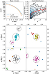 |
Fig. 2. Top left: mass function which defines our mock catalogue. The blue curve is Eq. (2) and the orange curve is the final mass distribution. At each value of 𝒩, the orange curve is the number of galaxies contained within the maximum integer number of groups with size 𝒩 allowed by the blue curve (see text). Top right: radial size of groups as a function of group membership. The black points are the mock galaxies and are bound by the dashed black lines. The value of the black solid line at 𝒩 = 2 is equal to σker: only pairs where the two galaxies are closer than about this value are grouped as pairs by TD-ENCLOSER (at 𝒩 = 2). We overlay 88357 groups with richness between 2 and 30 members from the Tempel et al. (2017) catalogue as a blue contour map. The median group radius for each group richness for the Tempel et al. (2017) catalogue is shown in red. Bottom: we show the four largest groups in the mock catalogue. Around each group of five or more members, the maximum radius is shown as a dashed circle. Each group is identified by a colour and marker. |
where α = −1.35, 𝒩 is the group membership, and A is a scale factor. We choose our break 𝒩0 to be 15 as it is simply half the maximum allowed group size. We use a scale factor A ≈ 282.510 so that nS(30) = 30 such that a group of 30 members has a mass of 30 in units of x. However, the statement nS(𝒩) = 𝒩 is only true for 𝒩 = 30 due to the shape of the function. As we require integer numbers of groups with membership 𝒩, we take the number of groups with membership 𝒩 as ⌊nS(𝒩)/𝒩⌋ where ⌊⌋ denotes floor.
To populate the box, we generate (xgrp, ygrp) coordinates for each group from a random uniform distribution within the limits of the box. We do not attempt to replicate the large scale structure of the cosmic web, as we are merely interested in assessing how the algorithm performs in a number of simple topologies. For each group with 𝒩mem > 1, we assign a radius  where fr is randomly chosen from a uniform distribution with range [ − 0.3, 0.3] (see the top right panel of Fig. 2). We choose 7 as an empirical factor so that roughly 50% of galaxy pairs are separated by 0.3 Mpc or less (so as to be picked up by TD-ENCLOSER). Clearly this simple prescription assumes that the area of a group is proportional to its membership. However, we compare this with the median group radius (r200) for galaxy groups in the Tempel et al. (2017) catalogue and find that our expression matches quite well with this. At the lower memberships, the Tempel et al. (2017) group radii distribution at fixed 𝒩 is more skewed towards larger radii than our randomly generated group radii. For each group, we randomly sample relative (xgal, ygal) coordinates for 𝒩 galaxies uniformly between [ − r, r]. When 𝒩 is large, this will naturally lead to a distribution which is peaked at the group centre. When 𝒩 is small, the groups will be less concentrated. If we had instead sampled the relative galaxy coordinates from a random Gaussian distribution, we would not expect a significant difference in the output. The final coordinate for a given galaxy is then (xgrp + xgal, ygrp + ygal).
The mock catalogue we have described is not intended to be a realistic representation of the cosmic web. Therefore, it comes attached with a strong caveat that the number of isolated galaxies in the catalogue is not calibrated to either observations or theory. Here we have assumed there is a constant occupation fraction of the dark matter halos such that the galaxy mass function is a simple scaling of the halo mass function. However, the occupation fraction is likely to vary significantly, especially at the low-mass end. This implies that the total fraction of isolated galaxies in the mock catalogue is much smaller than the fraction of isolated galaxies in reality and so it may be easier to find groups in the mock than in observations.
Generating a realistic mock catalogue would require a simulation, which would be far from trivial to do. The mock catalogue we have generated here is not intended to be a realistic simulation but rather a simple test case which contains crude approximations for galaxy groups. The purpose of this test is to determine how well TD-ENCLOSER performs when we know the true galaxy group assignments and so are able to carry out a comparison.
In the lower panel of Fig. 2, we show the four largest groups in our mock catalogue. Each group with five or more members is enclosed by a circle with a radius equal to the maximum radius allowed for each group. This panel explains why we do not necessarily recover the input distribution exactly. Firstly, as the coordinates of both galaxies and groups are randomly chosen, it is likely that some groups will overlap and become a single group, or even some isolated galaxies might lie embedded within another group. TD-ENCLOSER does not know the true input distribution. Furthermore, we have programmed TD-ENCLOSER to sensibly clip outliers and so some galaxies from large groups may be detached from their original groups.
Nevertheless, it is still useful to compare the mass function of the input with the mass function determined using the default parameters, even if individual galaxies are not in similar groups in both. As shown in Fig. 3, the ‘recovered’ mass function is not too dissimilar from the input mass function. The discrepancies are due to the reasons outlined above. In particular, the total mass contained within individual galaxies is more in the ‘recovered’ mass function compared to the input mass function, while the mass contained within galaxy pairs is less in the ‘recovered’ mass function compared to the input mass function. This is because our radial size prescription was calibrated such that approximately half of all galaxy pairs lie have a separation smaller than 0.3 Mpc (see top right panel of Fig. 2). Hence, we expect fewer galaxy pairs and more isolated galaxies in the ‘recovered’ distribution according to our prescription.
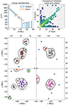 |
Fig. 3. Top left: mass function of the mock catalogue (described by a Schechter function) is shown in orange and the mass function of the groups found by TD-ENCLOSER is shown in blue. Top right: galaxy-wise comparison of the richness of their enclosing groups between the input and output catalogues. The colour in each cell represents the number of galaxies in that cell, where yellow or purple indicates a larger or smaller number respectively. Bottom: same as the bottom panel of Fig. 2, except that galaxies are coloured according to the groups which they have been assigned by TD-ENCLOSER. The contours are ρouter (black), 2.5ρouter = ρsaddle (dark grey) and 4ρouter (light grey). Isolated galaxies are shown as blue circles and galaxy pairs are shown as orange circles. The colours continue in sequence and the marker indicates the group size in multiples of 10: circles are between 1 and 10, squares are between 11 and 20, diamonds are between 21 and 30 and triangles are between 31 and 40. |
4.2. Testing parameter sensitivity
In order to check how the group assignments depend on each parameter, we vary the parameters σker, ρsaddle, ρpeak and Nmerge in turn and rerun TD-ENCLOSER on the mock catalogue. We do not perturb the values by a large amount because there are restrictions on each parameter, but also because we already have a good idea about what the default values should be. For example, we have already found σker = 0.3 Mpc gives the most faithful representation of the true galaxy distribution. We know from EH98 that ρouter does have a significant effect on the result and hence we do not vary this parameter at all. We could vary this parameter about 1.6 which may help improve the mass reconstruction, but we choose to keep it fixed to keep the degrees of freedom to a minimum. We could also vary σker with a finer granularity to find a more precise value that results in an improved group reconstruction. However we have chosen to limit our precision to 0.3 ± 0.05 Mpc for simplicity. Moreover, we have assumed a constant kernel width for all galaxies, whereas there would be a dependence on the stellar mass. We consider this level of precision to be consistent with this assumption. For the other three parameters, there are stricter constraints. ρsaddle cannot be equal to ρouter if it is to clip outliers effectively and in practice it should be at least 2ρouter. ρpeak must not be equal (or even very close) to ρsaddle regardless of the value of ρsaddle as this will split groups unnecessarily. We suggest that ρpeak − ρsaddle ≥ 0.25ρouter as a minimum separation. Finally, Nmerge must be greater than or equal to two, as at least two galaxies are required to calculate a mean. In the following test, we keep to these limits so that TD-ENCLOSER can operate as desired. If the results depend only weakly on each parameter, we can be confident in our ability to effectively assign galaxies to groups.
4.2.1. Test results
The results of our test are shown in Fig. 4, where for each panel, we change one parameter keeping all others the same. To indicate which parameter we are varying, we use the notation [vary(P)] where P is the parameter that is not set to the default value. If all parameters are set to the default values, then we use the shorthand [default]. Rather than show the mass function as in Fig. 3, we take the difference between the input group richness 𝒩 and the perturbed parameters (𝒩[vary(P)]) for each mock galaxy and compute the histogram for all mock galaxies. We are comparing the input from Fig. 2 with the output with Fig. 3 using different values for the free parameters. To give a complete picture, we could replace the x and y axis in the top-right panel of Fig. 3 with 𝒩[input] and 𝒩[vary(P)] respectively. However, this would give us twelve panels to present, three for each parameter. Instead, we show the difference in the richness distribution with varying parameters. The result is Fig. 4 where each panel corresponds to a parameter and each panel contains three histograms corresponding to each value we choose.
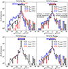 |
Fig. 4. Histograms illustrating how the group membership depends on the free parameters of TD-ENCLOSER. In each panel, three histograms are shown each corresponding to a particular set of parameter values. In each case, all but one of the values are set to the default. The parameter which is varied is indicated in the legend. The black histogram is the same in all panels, as this corresponds to the default values for all the parameters. In each panel, the x-axis is the difference between the richness of the group a particular galaxy belongs to in the recovered distribution using the chosen value for each parameter, and the richness of the group that the galaxy belongs to in the input catalogue. Finally, we indicate the inner 95% of each distribution with arrows coloured according to the corresponding histogram. |
We go through each panel of Fig. 4 in turn. Each histogram can be interpreted in the following way: if a single galaxy is near a group of 20 galaxies in the input mock catalogue, then when σker = 0.4, it becomes part of a new group of 21 members. In this case, ![$ \mathcal{N}^{[\mathrm{vary}(\sigma_{\mathrm{ker}})]}=\mathcal{N}^{[\mathrm{input}]}+1 $](/articles/aa/full_html/2023/07/aa36851-19/aa36851-19-eq4.gif) for 20 galaxies and
for 20 galaxies and ![$ \mathcal{N}^{[\mathrm{vary}(\sigma_{\mathrm{ker}})]}=\mathcal{N}^{[\mathrm{input}]}+20 $](/articles/aa/full_html/2023/07/aa36851-19/aa36851-19-eq5.gif) for one galaxy.
for one galaxy.
4.2.2. Varying σker
We select σker = 0.2, 0.3 and 0.4 Mpc. Of these three choices, we find that the distribution corresponding to σker = 0.3 Mpc is most balanced around zero. For this value of σker, we find that ∼61 % of galaxies lie in equally sized groups in the input group catalogue and in the output from TD-ENCLOSER. Comparing σker = 0.3 with σker = 0.2, we find that setting σker = 0.2 Mpc generally results in galaxies forming smaller groups in the first pass compared to σker = 0.3 Mpc. A small fraction of galaxies (∼1%) join larger groups due to the fact that by using a smaller kernel, some groups that would have reached ρpeak when σker = 0.3 would not have reached ρpeak when σker = 0.2. Hence, these groups would not have been clipped in the second pass with σker = 0.2 and therefore the galaxies which were clipped when σker = 0.3 have appeared to join a larger group, even though the kernel size has decreased. However, this occurrence is rare because ρpeak is close to ρsaddle. Conversely, setting σker = 0.4 Mpc results in more galaxies residing in larger groups compared to the default choice. Here, about 2% of galaxies join smaller groups because they are clipped when σker = 0.4 but not when σker = 0.3, and hence belong to a smaller group even though the kernel size has increased. The result is most sensitive to this parameter out of the four parameters as evidenced by the lower height of each peak at ![$ \mathcal{N}^{[\mathrm{vary}(\sigma_{\mathrm{ker}})]}-\mathcal{N}^{[\mathrm{input}]}=0 $](/articles/aa/full_html/2023/07/aa36851-19/aa36851-19-eq6.gif) (indicating no change) and the broad distribution.
(indicating no change) and the broad distribution.
4.2.3. Varying ρsaddle
We select ρsaddle = 3.6, 4.0 and 4.4. A value of ρsaddle = 3.6 tends to increase group sizes (and reduce the number of groups) as some galaxies are less likely to be clipped in the second pass than when ρsaddle = 4. This makes sense conceptually as all groups above ρpeak essentially grow and absorb nearby groups. A very small fraction of galaxies move to smaller groups which occurs when a small group is split up and one part joins a nearby large group and the other part then forms a small group. In total, 95% of galaxies change group membership by less than 3. Choosing a value of ρsaddle = 4.4 means that galaxies are more likely to be clipped from their original groups. Again, 95% of galaxies change group membership by less than 3.
4.2.4. Varying ρpeak
We select ρpeak = 4.4, 4.8 and 5.2. As seen in the third panel of Fig. 4, this is the parameter that the group membership is the least sensitive to. This is because varying ρpeak only changes which groups are clipped in the second pass and does not have any bearing on how much those groups are clipped. By lowering ρpeak, more groups are clipped. If ρpeak is increased compared to the default value, then fewer groups are clipped. In total, 95% of galaxies do not change group membership at all.
4.2.5. Varying Nmerge
We select Nmerge = 2, 4 and 8. Using Nmerge = 2, galaxies at the fringe of ρsaddle are more likely to be clipped during the second pass compared with Nmerge = 4. Hence, groups are more likely to be split up into a large subgroup and one or more smaller subgroups (extended blue tail in the fourth panel). Using Nmerge = 6 means that galaxies are less likely to be clipped (extended red tail in the fourth panel). Because this parameter is only relevant in the second pass, and then only when a group reaches ρpeak, the sensitivity of the result on Nmerge is less than that of σker and ρsaddle and only slightly more than ρpeak. This can be seen as 95% of galaxies change membership by 4 or less when Nmerge = 2, and by 1 or zero when Nmerge = 6.
4.3. TD-ENCLOSER running speed
Finally, in Fig. 5, we assess the speed of TD-ENCLOSER. As TD-ENCLOSER is designed to only consider the local environment close to a ‘target’ galaxy, it is not optimised for large sample sizes. We find that the elapsed time depends linearly on the sample size, taking approximately 5 seconds to iterate through 1000 galaxies using a 3 GHz CPU with 8 GB of RAM. We check to see if the speed varies with different choices in the parameters (not shown). We find that for N ≳ 100, where N is the number of galaxies in a fixed square window of sides 100 Mpc, choosing parameters that reduce the number of galaxies to consider in the second and third passes decreases the performance time. Of these, choosing a lower clipping threshold (ρsaddle) gives the largest reduction in speed because fewer galaxies are clipped. Choosing a larger Nmerge also reduces the number of galaxies to be clipped. Finally, by choosing a higher ρpeak, fewer groups are clipped in the second pass, although the improvement is minor overall.
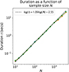 |
Fig. 5. Duration of a TD-ENCLOSER run as a function of sample size. All runs are performed within a box of 100 Mpc2. Three different runs are shown in orange, blue and green. The dashed line is the connecting line between the points at N = 100 and N = 1000 and is given in the legend. |
Choosing values that increases the number of galaxies to be considered after the first pass increases the time taken. The most significant increase is seen with ρsaddle, where an increase of 10% in ρsaddle results in a 10% increase in calculation time. Decreasing Nmerge by a factor of two compared to the default value only results in a 5% increase in performance time, and there is almost no change with ρpeak. ρsaddle produces the biggest changes overall to performance time.
5. Accounting for group multiplicity
As described in Sect. 3.2.1, TD-ENCLOSER defines a set of neighbours for each given galaxy: these neighbours fall within a box of 20 × 20 comoving Mpc and within a certain δz (corresponding to between ±300 km s−1 and ±3000 km s−1), centred on the given galaxy. In the ideal case of two nearby galaxies with exactly the same redshift, the set of neighbours would cover exactly the same δz , and so the two 2D density grids built at line 4 of Algorithm 1 would have the same values at the same RA-Dec positions. In the real world, two galaxies belonging to the same group will not have the same exact redshift, especially because of redshift space distortions, and so the set of neighbours entering in the boxes around the two galaxies might differ because the δz selection will be centred at slightly different z. This will possibly cause the algorithm to find slightly different groups using the two sets of neighbours, although the true underling galaxy distribution is the same. We refer to this issue as ‘group multiplicity’, that is when a galaxy might apparently belong to two slightly different groups if the set of neighbours is slightly different.
Take the following example: Suppose that a given galaxy group contains four MaNGA galaxies, [M1, M2, M3, M4], where each MaNGA galaxy (such as M1 with redshift z1) plays host to its own set of neighbours (M1 would host S1). Each set of neighbours is found by running TD-ENCLOSER with the target galaxy as one of the MaNGA galaxies. To avoid ambiguity, the term ‘set’ in this context does not refer to the set of galaxies from which the groups are found, but rather refers to the set of neighbours found by TD-ENCLOSER. Hence, we find four sets of galaxies. In the case that each MaNGA galaxy has the same redshift, so that z1 = z2 = z3 = z4, the sets will be identical, and so we can randomly select one of the sets to represent all four. However, we may be presented with a case where z1 ≠ z2 ≠ z3 ≠ z4 and so the four set of galaxies may not be equal. In fact, it is possible that not all four MaNGA galaxies will appear in all four sets. In another example, a MaNGA galaxy can appear on the outskirts of a large cluster with hundreds of member galaxies, but can also appear as a small group. In these cases, we need to choose a subset to represent the intrinsic groups so that each MaNGA galaxy appears only once in our catalogue. In other words, given a suite of sets that share MaNGA galaxies, we need to choose a subset of those sets that satisfies the constraint that no two sets in the subset share any MaNGA galaxies. We then treat these final sets as groups.
We achieve this aim using the following steps. Step 1: We select N1 MaNGA galaxies which are contained within set S1. Step 2: We select N2 sets that contain at least one of the MaNGA galaxies belonging to set S1. N2 may be larger than N1. Step 3: We select N3 MaNGA galaxies that are found in the N2 set identified in step 2. Step 4: If N3 > N1, then we repeat steps 1.−3. selecting the set of N3 MaNGA galaxies which are found in set N2. If N3 = N1, we move onto step 5. Step 5: We select all sets that are larger than half the maximum richness, 𝒩max, of the final sets. This step ensures we are likely to select duplicates or variations of the same large group, deselecting nearby small groups and isolated galaxies that are otherwise connected to the large group. Step 6: Of the subset of sets that satisfy 𝒩 > 𝒩max/2, we calculate the median redshift of the host galaxies in the subset. Step 7: We select the set SM which encloses the MaNGA galaxy with the median redshift and assign this set to the final selection. If there are more than one MaNGA galaxies at the median redshift, we randomly select one. Step 8: We remove all sets which contain the same MaNGA galaxies as set SM from our final selection. Step 9: If there are remaining sets that do not share any MaNGA galaxies in common with set SM, we randomly select non-unique galaxies within the remaining sets11, and repeat step 8. Step 10: We repeat step 9. until all MaNGA galaxies are assigned to one set only.
We illustrate this selector algorithm in Fig. 6. We start with set S1 and find that it hosts five MaNGA galaxies (step 1.). We then check all other sets and find five more sets that contain at least one of these five MaNGA galaxies (step 2.). Two of these (sets S5 and S6) contain MaNGA galaxies that are not found in set S1, and so we search for all sets that contain these new MaNGA galaxies (step 3.). We find four new sets that do not contain any of the original five MaNGA galaxies, but are linked to set S1 by a chain of MaNGA galaxies (step 4.). As we do not find any more sets containing these new MaNGA galaxies, the tree stops growing here.
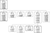 |
Fig. 6. Finding unique groups. Here we show an example where 10 galaxy sets are connected by a network of MaNGA galaxies. For each set, we give the richness 𝒩 and the redshift of the ‘host’ MaNGA galaxy. The starting set is set S1, and its member galaxies are emphasised in bold. The final representative sets selected by the selector are sets S1, S9 and S10 which are indicated by thick borders. These three sets do not share any MaNGA galaxies, but may share SDSS galaxies not observed with MaNGA (see text). This example has many possible solutions (see the text for details). |
Following step 4. above, we select all sets that are richer than half the maximum richness. In this example, set S5 is the richest set with 56 members, and so we select sets S1, S5, S6, S8 and S10. Of these five sets, we select the set with the median redshift, which in this case is set S10 (steps 6. and 7.). This is the first set to make the final selection. We deselect all sets that share at least one MaNGA galaxy in common with set S10, namely sets S5, S7 and S8 (step 8.). We randomly select one of the remaining sets, which happens to be set S1 (step 9.). The only remaining set that does not share any MaNGA galaxies in common with set S1 is set S9, and so the final selection contains sets S1, S9 and S10 (step 10.). We could also select sets S2, S3, S4, S6, S9 in step 9., in which case the final selection would be slightly different.
There are a few alternative ways we could use to select the representative set(s). For example, we could take the largest set found as that is most likely to contain all of the MaNGA galaxies. However, that may bias us towards larger groups. We could also randomly select the representative set from all possible sets, but that may select a small set instead of a larger set just by chance. For a large group with many MaNGA galaxies, we may miss a substantial fraction of the group if we were to select MaNGA galaxies at the extreme velocities. Therefore, by choosing a set based on the median redshift of the MaNGA galaxies, we expect the cylinder to encompass the ‘true’ velocity extent of the group.
The group selector algorithm only solves for unique MaNGA galaxies. We do not solve for MaNGA and SDSS galaxies, or in other words, we do not find sets which do not share any galaxies, MaNGA or SDSS, because there may be no solutions to that problem. The final sets chosen in the above example have a total membership of 76 galaxies, but two SDSS galaxies are members of two of the sets, meaning that the total number of unique galaxies (MaNGA and SDSS) is 74 (see groups 2755, 4375 and 4379 in the catalogue from Paper II). We are making the assumption that by selecting sets which do not share MaNGA galaxies, we are minimising the duplicity of SDSS galaxies. To optimise the process, we could add an extra constraint that the final sets should share the minimum number of SDSS (non-MaNGA) galaxies possible. However, we would not be able to eliminate the duplicity completely, and we would add an extra layer of complexity to the process. Taking the catalogue as a whole, it is not totally unbiased since there are some duplicate galaxies (see Sect. 4.4 of Paper II).
Finally, in steps 7. and 9., we use a random selection to select a MaNGA galaxy. We could in both cases select the MaNGA galaxy with the highest ρ. This would remove the non-deterministic element of the group selector algorithm, and would prevent some sets ever being chosen. If we wanted to repeat the analysis in Paper III with a slightly different final group selection, this algorithm as is would allow that, whereas if we were to choose based on the highest ρ, we would always return the same groups. In practice, our redshift precision is to 4 significant figures, so the chances of two MaNGA galaxies sharing a redshift in a small group with only a handful of galaxies is small. The random step is only likely needed where there are tens of MaNGA galaxies in close proximity where maybe two or three have the same redshift.
It is possible that some MaNGA galaxies will not make it into the final selection, depending on the exact galaxy configuration in three dimensional space. If we take our earlier example of four MaNGA galaxies, but split them into three sets of [M1, M2, M3] and one set of [M2, M3, M4], then according to our random selection, M4 is likely to be excluded. To illustrate this point further, we take an example from the galaxy groups given in Paper II. In Fig. 7, we show the MaNGA galaxies from three overlapping groups. As we only consider MaNGA galaxies, we do not show the galaxies which are not in MaNGA. In our final catalogue, we require that each MaNGA galaxy belongs to only one group. Hence, we apply our selector algorithm to randomly select one of these groups. The galaxies which belong to the group which is selected are highlighted with a black border. The two groups which are not selected are shown in blue and red. Of the MaNGA galaxies that belong to the blue group, only one is not part of the final selected group. Likewise, of the two MaNGA galaxies that belong to the red group, only one of them does not belong to the final group. Of the three groups shown, the two large groups have an equal chance of being selected, while the red group with only two galaxies has no chance of being selected (because of step. 5). As a result, two MaNGA galaxies are not assigned to any groups in the final selection. We find that out of 4028 MaNGA galaxies that lie in sets with a median redshift z ≤ 0.08, 137 (∼3.4%) are not included in the final catalogue due to similar scenarios as the one shown in Fig. 7. The reason for this is that TD-ENCLOSER tends to assign these galaxies to small groups or to the fringes of larger groups, and so when the group multiplicity is accounted for, they do not make it into the final ‘complete’ group catalogue in Paper II.
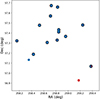 |
Fig. 7. Example of group multiplicity. We plot the RA-Dec distribution of three galaxy groups which share at least one MaNGA galaxy with one of the other of the three groups. There are two large groups, one indicated with a blue marker, and the other with a black empty circle. There is also a small group indicated with a red marker (lower right). There is one MaNGA galaxy that belongs to all three groups. The group selector algorithm has selected the group of galaxies indicated with the black empty marker. The mean redshift of these galaxies is 0.028. |
We note that the motivation for developing this algorithm to address the multiplicity (steps 1–10 in this section) is in no way related to any functionality of TD-ENCLOSER. Instead, it is designed to address the inherent uncertainty in the sample constructed in Paper II.
6. Conclusions
In Sect. 3, we introduced a new group finder algorithm (TD-ENCLOSER) which has some features in common with the HOP method of EH98 (see Algorithm 1), but is based on an entirely different method. Its main function is to assign galaxies to regions of high density, before clipping outliers and forming new groups from those outliers (Fig. 1). TD-ENCLOSER is different to most other group-finder algorithms in that it is used to discover which group encloses a particular galaxy of interest. It is not designed to produce large group catalogues of hundreds of thousands of galaxies but can be used to obtain the local galaxy distribution. It works on the simple assumption that the gradient along a one-dimensional straight line between two points encodes the local two-dimensional topology. If the gradient of the connecting line between a galaxy and a nearby peak does not fall below a small noise threshold ϵ, and if the galaxy is in a sufficiently dense environment, then we assign the galaxy to that peak. If the galaxy satisfies the threshold to be in a group but is sufficiently far enough from the peak to be near the outskirts, it is ejected from the peak after which it seeks to join a new, smaller group. As with any algorithm, there will inevitably be anomalies, especially when the contour topology is complex. However, we have shown in this work that TD-ENCLOSER performs reliably enough to be used on real life cases. As such, we have applied TD-ENCLOSER to thousands of galaxies (see Paper II for an overview and Paper IV for a few key examples).
In Sect. 4, we tested TD-ENCLOSER on a mock catalogue of galaxies using a Schechter mass function (Schechter 1976) to define the group membership (Fig. 2). While we did not aim to reproduce exactly the input distribution, we found that we could match the input mass function with reasonable accuracy (top left panel of Fig. 3). The reason for the discrepancy is that many pairs are broken up (by design) and a small percentage of individual galaxies can dramatically change their group membership (top right panel of Fig. 3). We found that of the four parameters where we have some freedom to choose the default values, TD-ENCLOSER is reasonably insensitive to all but one of them (Fig. 4). Again, individual galaxies can change group membership dramatically depending on the choice of parameters, but the fraction of galaxies with large changes in group membership is small. The highest sensitivity is towards σker, which is a known feature of KDE methods. We checked the speed of operation and found that it increases linearly with the sample size (Fig. 5). The parameter that introduces the most variation is ρsaddle where a variation of 10% results in a similar change in performance time.
In preparation for the task of constructing the group catalogue in Paper II, we have developed a simple procedure to select one or more representative groups of a set of duplicates linked by MaNGA galaxies (see Sect. 5). We select representative sets using knowledge about the group size while incorporating a random selection to ensure we are not biased towards any particular sets.
A comprehensive list of galaxy group catalogues can be found here: https://go.nasa.gov/30Mz1PI.
The name TD-ENCLOSER encapsulates the general idea behind our algorithm in that it considers galaxies by their density in descending order, or in other words, top-down (TD). ENCLOSER refers to the fact that the algorithm finds the group that encloses a particular galaxy. As the algorithm was developed with a specific astronomical application in mind, we give it an unofficial acronym in the spirit of so many other acronyms in astronomy: Top Down-EfficieNt loCaL neighbOur SEarcheR.
Consider four sets: [M1, M2, M3], [M1], [M2] and [M3]. If we randomly select by set, then the set containing three MaNGA galaxies has only a 25% chance of being selected. If we choose by MaNGA galaxy and select its enclosing set, then the set containing three MaNGA galaxies has a 50% chance of being selected. We choose to select using the latter method in step 9.
Acknowledgments
We thank the anonymous referee for their detailed and constructive comments which led to the significant improvement of this manuscript. Funding for the Sloan Digital Sky Survey IV has been provided by the Alfred P. Sloan Foundation, the U.S. Department of Energy Office of Science, and the Participating Institutions. SDSS acknowledges support and resources from the Center for High-Performance Computing at the University of Utah. The SDSS website is www.sdss.org. SDSS is managed by the Astrophysical Research Consortium for the Participating Institutions of the SDSS Collaboration including the Brazilian Participation Group, the Carnegie Institution for Science, Carnegie Mellon University, the Chilean Participation Group, the French Participation Group, Harvard-Smithsonian Center for Astrophysics, Instituto de Astrofísica de Canarias, The Johns Hopkins University, Kavli Institute for the Physics and Mathematics of the Universe (IPMU)/University of Tokyo, Lawrence Berkeley National Laboratory, Leibniz Institut für Astrophysik Potsdam (AIP), Max-Planck-Institut für Astronomie (MPIA Heidelberg), Max-Planck-Institut für Astrophysik (MPA Garching), Max-Planck-Institut für Extraterrestrische Physik (MPE), National Astronomical Observatories of China, New Mexico State University, New York University, University of Notre Dame, Observatório Nacional/MCTI, The Ohio State University, Pennsylvania State University, Shanghai Astronomical Observatory, United Kingdom Participation Group, Universidad Nacional Autónoma de México, University of Arizona, University of Colorado Boulder, University of Oxford, University of Portsmouth, University of Utah, University of Virginia, University of Washington, University of Wisconsin, Vanderbilt University, and Yale University. This publication makes use of data products from the Two Micron All Sky Survey, which is a joint project of the University of Massachusetts and the Infrared Processing and Analysis Center/California Institute of Technology, funded by the National Aeronautics and Space Administration and the National Science Foundation.
References
- Aguado, D. S., Ahumada, R., Almeida, A., et al. 2019, ApJS, 240, 23 [Google Scholar]
- Belfiore, F., Westfall, K. B., Schaefer, A., et al. 2019, AJ, 158, 160 [CrossRef] [Google Scholar]
- Bertschinger, E., & Gelb, J. M. 1991, Comput. Phys., 5, 164 [NASA ADS] [CrossRef] [Google Scholar]
- Blanton, M. R., & Moustakas, J. 2009, ARA&A, 47, 159 [Google Scholar]
- Blanton, M. R., Eisenstein, D., Hogg, D. W., Schlegel, D. J., & Brinkmann, J. 2005, ApJ, 629, 143 [Google Scholar]
- Blanton, M. R., Bershady, M. A., Abolfathi, B., et al. 2017, AJ, 154, 28 [Google Scholar]
- Bundy, K., Bershady, M. A., Law, D. R., et al. 2015, ApJ, 798, 7 [Google Scholar]
- Carreira-Perpiñán, M. 2015, ArXiv e-prints [arXiv:1503.00687] [Google Scholar]
- Cheng, Y. 1995, IEEE Trans. Pattern Anal. Mach. Intell., 17, 790 [CrossRef] [Google Scholar]
- Cherinka, B., Andrews, B. H., Sánchez-Gallego, J., et al. 2019, AJ, 158, 74 [CrossRef] [Google Scholar]
- Colless, M., Dalton, G., Maddox, S., et al. 2001, MNRAS, 328, 1039 [Google Scholar]
- Davis, M., Efstathiou, G., Frenk, C. S., & White, S. D. M. 1985, ApJ, 292, 371 [Google Scholar]
- Doi, M., Tanaka, M., Fukugita, M., et al. 2010, AJ, 139, 1628 [NASA ADS] [CrossRef] [Google Scholar]
- Driver, S. P., Norberg, P., Baldry, I. K., et al. 2009, Astron. Geophys., 50, 5.12 [NASA ADS] [CrossRef] [Google Scholar]
- Driver, S. P., Hill, D. T., Kelvin, L. S., et al. 2011, MNRAS, 413, 971 [Google Scholar]
- Drory, N., MacDonald, N., Bershady, M. A., et al. 2015, AJ, 149, 77 [CrossRef] [Google Scholar]
- Eisenstein, D. J., & Hut, P. 1998, ApJ, 498, 137 [NASA ADS] [CrossRef] [Google Scholar]
- Eke, V. R., Baugh, C. M., Cole, S., et al. 2004, MNRAS, 348, 866 [NASA ADS] [CrossRef] [Google Scholar]
- Fukugita, M., Ichikawa, T., Gunn, J. E., et al. 1996, AJ, 111, 1748 [Google Scholar]
- Gelb, J. M., & Bertschinger, E. 1994, ApJ, 436, 467 [NASA ADS] [CrossRef] [Google Scholar]
- Geller, M. J., & Huchra, J. P. 1983, ApJS, 52, 61 [NASA ADS] [CrossRef] [Google Scholar]
- Graham, M. T., Cappellari, M., Bershady, M. A., & Drory, N. 2019a, A&A, submitted [arXiv:1910.05136] [Google Scholar]
- Graham, M. T., Cappellari, M., Bershady, M. A., & Drory, N. 2019b, A&A, submitted [arXiv:1910.05139] [Google Scholar]
- Graham, M. T., Cappellari, M., Bershady, M. A., & Drory, N. 2019c, A&A, submitted [arXiv:1911.06103] [Google Scholar]
- Gunn, J. E., Carr, M., Rockosi, C., et al. 1998, AJ, 116, 3040 [NASA ADS] [CrossRef] [Google Scholar]
- Gunn, J. E., Siegmund, W. A., Mannery, E. J., et al. 2006, AJ, 131, 2332 [NASA ADS] [CrossRef] [Google Scholar]
- Hinneburg, A., & Gabriel, H. H. 2007, in Advances in Intelligent Data Analysis VII, eds. M. R. Berthold, J. Shawe-Taylor, & N. Lavrač (Berlin, Heidelberg: Springer), 70 [Google Scholar]
- Hinneburg, A., & Keim, D. A. 1998, KDD, 98, 58 [Google Scholar]
- Huchra, J. P., & Geller, M. J. 1982, ApJ, 257, 423 [NASA ADS] [CrossRef] [Google Scholar]
- Huchra, J. P., Macri, L. M., Masters, K. L., et al. 2012, ApJS, 199, 26 [Google Scholar]
- Jones, D. H., Read, M. A., Saunders, W., et al. 2009, MNRAS, 399, 683 [Google Scholar]
- Knebe, A., Pearce, F. R., Lux, H., et al. 2013, MNRAS, 435, 1618 [NASA ADS] [CrossRef] [Google Scholar]
- Law, D. R., Yan, R., Bershady, M. A., et al. 2015, AJ, 150, 19 [CrossRef] [Google Scholar]
- Law, D. R., Cherinka, B., Yan, R., et al. 2016, AJ, 152, 83 [Google Scholar]
- Merchán, M., & Zandivarez, A. 2002, MNRAS, 335, 216 [CrossRef] [Google Scholar]
- Merchán, M. E., & Zandivarez, A. 2005, ApJ, 630, 759 [CrossRef] [Google Scholar]
- Miller, C. J., Nichol, R. C., Reichart, D., et al. 2005, AJ, 130, 968 [Google Scholar]
- Muñoz-Cuartas, J. C., & Müller, V. 2012, MNRAS, 423, 1583 [CrossRef] [Google Scholar]
- Parzen, E. 1962, Ann. Math. Stat., 33, 1065 [Google Scholar]
- Planck Collaboration XIII. 2016, A&A, 594, A13 [NASA ADS] [CrossRef] [EDP Sciences] [Google Scholar]
- Robotham, A. S. G., Norberg, P., Driver, S. P., et al. 2011, MNRAS, 416, 2640 [NASA ADS] [CrossRef] [Google Scholar]
- Schechter, P. 1976, ApJ, 203, 297 [Google Scholar]
- Scott, D. W. 1992, Multivariate Density Estimation (Wiley) [Google Scholar]
- Smee, S. A., Gunn, J. E., Uomoto, A., et al. 2013, AJ, 146, 32 [Google Scholar]
- Springel, V., White, S. D. M., Tormen, G., & Kauffmann, G. 2001, MNRAS, 328, 726 [Google Scholar]
- Tago, E., Einasto, J., Saar, E., et al. 2008, A&A, 479, 927 [NASA ADS] [CrossRef] [EDP Sciences] [Google Scholar]
- Tago, E., Saar, E., Tempel, E., et al. 2010, A&A, 514, A102 [NASA ADS] [CrossRef] [EDP Sciences] [Google Scholar]
- Tempel, E., Tago, E., & Liivamägi, L. J. 2012, A&A, 540, A106 [CrossRef] [EDP Sciences] [Google Scholar]
- Tempel, E., Tamm, A., Gramann, M., et al. 2014, A&A, 566, A1 [NASA ADS] [CrossRef] [EDP Sciences] [Google Scholar]
- Tempel, E., Kipper, R., Tamm, A., et al. 2016, A&A, 588, A14 [NASA ADS] [CrossRef] [EDP Sciences] [Google Scholar]
- Tempel, E., Tuvikene, T., Kipper, R., & Libeskind, N. I. 2017, A&A, 602, A100 [NASA ADS] [CrossRef] [EDP Sciences] [Google Scholar]
- Wake, D. A., Bundy, K., Diamond-Stanic, A. M., et al. 2017, AJ, 154, 86 [Google Scholar]
- Weinberg, D. H., Hernquist, L., & Katz, N. 1997, ApJ, 477, 8 [NASA ADS] [CrossRef] [Google Scholar]
- Westfall, K. B., Cappellari, M., Bershady, M. A., et al. 2019, AJ, 158, 231 [Google Scholar]
- Xie, C., Chang, J., & Song, Y. 2007, in Proceedings of the 2nd International Conference on Scalable Information Systems, 60 [Google Scholar]
- Xie, C., Song, Y., & Liu, Z. 2010, J. Inf. Comput. Sci., 7, 135 [Google Scholar]
- Yan, R., Bundy, K., Law, D. R., et al. 2016a, AJ, 152, 197 [Google Scholar]
- Yan, R., Tremonti, C., Bershady, M. A., et al. 2016b, AJ, 151, 8 [Google Scholar]
- Yang, X., Mo, H. J., van den Bosch, F. C., & Jing, Y. P. 2005, MNRAS, 356, 1293 [Google Scholar]
- Yang, X., Mo, H. J., van den Bosch, F. C., et al. 2007, ApJ, 671, 153 [Google Scholar]
- York, D. G., Adelman, J., Anderson, Jr., J. E., et al. 2000, AJ, 120, 1579 [NASA ADS] [CrossRef] [Google Scholar]
All Tables
All Figures
|
Fig. 1. One-dimensional visualisation of the group finder algorithm TD-ENCLOSER introduced in this section. The points in the three panels are identical and each point represents a galaxy. Galaxies belonging to the same group as coloured accordingly. The contour levels from bottom up are ρouter (solid), ρsaddle (dashed) and ρpeak (dotted). The outcome of the first pass is shown in the first panel, where galaxies are assigned to groups based only on the contour morphology, shown as the grey curve. In the second pass, outliers are disconnected from their groups based on the density of their Nmerge − 1 neighbours and are tagged as isolated. In the third pass, each ejected galaxy is assigned to a new group. All galaxies which were not clipped in the second pass are shown as faint to indicate that they are considered to be absent in the third pass. |
| In the text | |
|
Fig. 2. Top left: mass function which defines our mock catalogue. The blue curve is Eq. (2) and the orange curve is the final mass distribution. At each value of 𝒩, the orange curve is the number of galaxies contained within the maximum integer number of groups with size 𝒩 allowed by the blue curve (see text). Top right: radial size of groups as a function of group membership. The black points are the mock galaxies and are bound by the dashed black lines. The value of the black solid line at 𝒩 = 2 is equal to σker: only pairs where the two galaxies are closer than about this value are grouped as pairs by TD-ENCLOSER (at 𝒩 = 2). We overlay 88357 groups with richness between 2 and 30 members from the Tempel et al. (2017) catalogue as a blue contour map. The median group radius for each group richness for the Tempel et al. (2017) catalogue is shown in red. Bottom: we show the four largest groups in the mock catalogue. Around each group of five or more members, the maximum radius is shown as a dashed circle. Each group is identified by a colour and marker. |
| In the text | |
|
Fig. 3. Top left: mass function of the mock catalogue (described by a Schechter function) is shown in orange and the mass function of the groups found by TD-ENCLOSER is shown in blue. Top right: galaxy-wise comparison of the richness of their enclosing groups between the input and output catalogues. The colour in each cell represents the number of galaxies in that cell, where yellow or purple indicates a larger or smaller number respectively. Bottom: same as the bottom panel of Fig. 2, except that galaxies are coloured according to the groups which they have been assigned by TD-ENCLOSER. The contours are ρouter (black), 2.5ρouter = ρsaddle (dark grey) and 4ρouter (light grey). Isolated galaxies are shown as blue circles and galaxy pairs are shown as orange circles. The colours continue in sequence and the marker indicates the group size in multiples of 10: circles are between 1 and 10, squares are between 11 and 20, diamonds are between 21 and 30 and triangles are between 31 and 40. |
| In the text | |
|
Fig. 4. Histograms illustrating how the group membership depends on the free parameters of TD-ENCLOSER. In each panel, three histograms are shown each corresponding to a particular set of parameter values. In each case, all but one of the values are set to the default. The parameter which is varied is indicated in the legend. The black histogram is the same in all panels, as this corresponds to the default values for all the parameters. In each panel, the x-axis is the difference between the richness of the group a particular galaxy belongs to in the recovered distribution using the chosen value for each parameter, and the richness of the group that the galaxy belongs to in the input catalogue. Finally, we indicate the inner 95% of each distribution with arrows coloured according to the corresponding histogram. |
| In the text | |
|
Fig. 5. Duration of a TD-ENCLOSER run as a function of sample size. All runs are performed within a box of 100 Mpc2. Three different runs are shown in orange, blue and green. The dashed line is the connecting line between the points at N = 100 and N = 1000 and is given in the legend. |
| In the text | |
|
Fig. 6. Finding unique groups. Here we show an example where 10 galaxy sets are connected by a network of MaNGA galaxies. For each set, we give the richness 𝒩 and the redshift of the ‘host’ MaNGA galaxy. The starting set is set S1, and its member galaxies are emphasised in bold. The final representative sets selected by the selector are sets S1, S9 and S10 which are indicated by thick borders. These three sets do not share any MaNGA galaxies, but may share SDSS galaxies not observed with MaNGA (see text). This example has many possible solutions (see the text for details). |
| In the text | |
|
Fig. 7. Example of group multiplicity. We plot the RA-Dec distribution of three galaxy groups which share at least one MaNGA galaxy with one of the other of the three groups. There are two large groups, one indicated with a blue marker, and the other with a black empty circle. There is also a small group indicated with a red marker (lower right). There is one MaNGA galaxy that belongs to all three groups. The group selector algorithm has selected the group of galaxies indicated with the black empty marker. The mean redshift of these galaxies is 0.028. |
| In the text | |
Current usage metrics show cumulative count of Article Views (full-text article views including HTML views, PDF and ePub downloads, according to the available data) and Abstracts Views on Vision4Press platform.
Data correspond to usage on the plateform after 2015. The current usage metrics is available 48-96 hours after online publication and is updated daily on week days.
Initial download of the metrics may take a while.