| Issue |
A&A
Volume 673, May 2023
|
|
|---|---|---|
| Article Number | A63 | |
| Number of page(s) | 15 | |
| Section | Extragalactic astronomy | |
| DOI | https://doi.org/10.1051/0004-6361/202345962 | |
| Published online | 05 May 2023 | |
Non-parametric galaxy morphology from stellar and nebular emission with the CALIFA sample⋆
1
Sterrenkundig Observatorium Universiteit Gent, Krijgslaan 281 S9, 9000 Gent, Belgium
e-mail: This email address is being protected from spambots. You need JavaScript enabled to view it.
2
Osservatorio Astrofisico di Arcetri, Largo Enrico Fermi 5, 50125 Firenze, Italy
3
Kavli Institute for Cosmology, University of Cambridge, Madingley Road, Cambridge CB3 0HA, UK
4
Cavendish Laboratory – Astrophysics Group, University of Cambridge, 19 JJ Thomson Avenue, Cambridge CB3 0HE, UK
Received:
20
January
2023
Accepted:
2
March
2023
Abstract
Aims. We present a non-parametric morphology analysis of the stellar continuum and nebular emission lines for a sample of local galaxies. We explore the dependence of the various morphological parameters on wavelength and morphological type. Our goal is to quantify the difference in morphology between the stellar and nebular components.
Methods. We derived the non-parametric morphological indicators of 364 galaxies from the Calar Alto Legacy Integral Field Area (CALIFA) Survey. To calculate those indicators, we applied the StatMorph package on the high-quality integral field spectroscopic data cubes, as well as to the most prominent nebular emission-line maps, namely [O III]λ5007, Hα, and [N II]λ6583.
Results. We show that the physical size of galaxies, M20 index, and concentration have a strong gradient from blue to red optical wavelengths. We find that the light distribution of the nebular emission is less concentrated than the stellar continuum. A comparison between the non-parametric indicators and the galaxy physical properties revealed a very strong correlation of the concentration with the specific star formation rate and morphological type. Furthermore, we explore how the galaxy inclination affects our results. We find that edge-on galaxies show a more rapid change in physical size and concentration with increasing wavelength due to the increase in the optical free path.
Conclusions. We conclude that the apparent morphology of galaxies originates from the pure stellar distribution, but the morphology of the interstellar medium presents differences with respect to the morphology of the stellar component. Our analysis also highlights the importance of dust attenuation and galaxy inclination in the measurement of non-parametric morphological indicators, especially in the wavelength range 4000−5000 Å.
Key words: galaxies: structure / galaxies: spiral / galaxies: elliptical and lenticular, cD / galaxies: ISM
Data are only available at the CDS via anonymous ftp to cdsarc.cds.unistra.fr (130.79.128.5) or via https://cdsarc.cds.unistra.fr/viz-bin/cat/J/A+A/673/A63
© The Authors 2023
 Open Access article, published by EDP Sciences, under the terms of the Creative Commons Attribution License (https://creativecommons.org/licenses/by/4.0), which permits unrestricted use, distribution, and reproduction in any medium, provided the original work is properly cited.
This article is published in open access under the Subscribe to Open model. This email address is being protected from spambots. You need JavaScript enabled to view it. to support open access publication.
1. Introduction
One of the fundamental characteristics that we use to describe galaxies is their morphology, which can provide important clues about their formation and secular evolution. For example, processes such as in situ star formation or merging events can be traced by quantifying the structure and morphology of a galaxy (Conselice 2014). The simplest method of classifying galaxies is through a visual inspection of their apparent morphology (de Vaucouleurs 1959; Sandage 2005; Lintott et al. 2011). In that case galaxies can be segregated into four broad populations: ellipticals, lenticulars, spirals, and irregulars. Of course, each galaxy group can be further divided into sub-groups, for instance spirals can be with or without a bar structure. Usually a numerical value is assigned to each class of galaxy (Hubble stage T) ranging from −5 to +10, with negative numbers corresponding to ellipticals and lenticulars (early types) and positive numbers to spirals and irregulars (late types).
A more quantitative technique to measure galaxy structure is by fitting the surface brightness distribution of galaxies with a general Sérsic (1963) profile (Peng et al. 2010; Simard et al. 2011), described by three free parameters: the Sérsic index n, the effective radius enclosing half of the light within a galaxy (Re), and the effective surface brightness (μe). From the Sérsic index, it is possible to characterise if a galaxy is disk-like (n < 2) or bulge-dominated (n ≥ 2). Many studies have investigated the dependence of galaxy structure on wavelength by fitting Sérsic profiles in various optical and near-infrared (NIR) broad-band images (e.g. La Barbera et al. 2010; Kelvin et al. 2012; Häußler et al. 2013; Vulcani et al. 2014). Despite the discrete nature of broad-band photometry, those studies found a smooth transition of the structural parameters with wavelength for the early-type galaxies, and a more intense change for the late types. The reported trends can be attributed to the stellar population age and metallicity gradients, as well as dust attenuation effects. Lastly, this method was applied in the far-infrared Herschel bands by Mosenkov et al. (2019), who found a modest dependence of the Sérsic index on wavelength.
Another method to quantify galaxy morphology is by making use of non-parametric indicators. There are two commonly used sets of non-parametric properties: the Gini–M20 indices (Abraham et al. 2003; Lotz et al. 2004) and the concentration–asymmetry–smoothness (CAS) system (Conselice 2003). The advantages of measuring those indicators is (1) that they do not impose any functional form on a galaxy’s surface brightness distribution, and (2) that they can be applied to any galaxy image, regardless of wavelength or redshift. Therefore, measuring these parameters is ideal to capture the underlying morphology of the different galaxy components.
Previous studies have mainly focussed on the stellar distribution and the application of non-parametric indicators on optical and NIR galaxy images (Lotz et al. 2006; Huertas-Company et al. 2009; Holwerda et al. 2014; Conselice et al. 2009; Conselice 2014; Psychogyios et al. 2016; Rodriguez-Gomez et al. 2019). Other applications include the measurement of galaxy structure from HI maps (Holwerda et al. 2011; Gebek et al. 2023) and CO data (Davis et al. 2022). Muñoz-Mateos et al. (2009) extended the study of non-parametric morphology to the dust component in the far-infrared (FIR) regime, using the Spitzer MIPS 70 and 160 μm images. Baes et al. (2020) presented, for the first time, a multi-wavelength study of the non-parametric morphology of nine nearby spiral galaxies, in order to consistently measure the variation of galaxy structure in the UV-submm wavelength range.
The application of non-parametric morphological parameters to broad-band images only allows to recover the average properties of galaxies in a specific waveband, missing significant fraction of the nuanced information of the different stellar populations and interstellar medium (ISM). Indeed, the ISM is a very complex environment where the fundamental physical processes transpire within galaxies as a consequence of cosmologic evolution. An important asset towards that goal is deciphering the spectrum of a galaxy. A single spectrum contains information not only of the age of stellar populations, but also of the star formation rate (SFR), stellar and gas-phase metallicity, dust content, and chemical abundances. Furthermore, a spectrum can reveal physical processes that shape the ISM such as shocks from massive stellar winds, feedback from an active galactic nucleus (AGN), the strength of the stellar radiation field, and gas collisions due to merging events (see review by Kewley et al. 2019).
In recent years, the advancement of Integral Field Spectroscopy (IFS) has enabled the formation of large surveys of galaxies, in particular ATLAS3D (Cappellari et al. 2011), Calar Alto Legacy Integral Field Area (CALIFA; Sánchez et al. 2012, 2016; Walcher et al. 2014), Mapping Nearby Galaxies at Apache Point Observatory (MaNGA; Bundy et al. 2015) and Sydney-AAO Multi-object Integral field (SAMI; Bryant et al. 2015) Galaxy survey. Those surveys not only increased the sample sizes and wavelength coverage of the Integral Field Units (IFUs), but also improved in spatial resolution (although the field of view still remains quite small). An interesting aspect of the available, spatially resolved spectra, that has remained fairly unexplored, is the variability of galaxy morphology as a function of wavelength.
As previously stated, most morphology indicator studies have been based on broad-band images containing a mix of stellar continuum emission and gas line emission. By using IFU data we can mask the disturbing contribution of nebular line emission, and calculate the morphological indicators from the pure stellar emission only. In particular the wavelength dependence of these pure stellar emission indicators is an interesting thing to study, as different aspects contribute to it: stellar population gradients and gradients in dust attenuation. Conversely, we can also isolate the nebular line emission and study (for the first time systematically) the morphology of the ionised gas and compare that to the morphology of the stellar emission.
The goal of this paper is to extract the non-parametric morphological statistics from IFU frames, corresponding to the stellar continuum and to different spectral features in the optical regime, for a large number of galaxies. The CALIFA (Sánchez et al. 2012, 2016; Walcher et al. 2014) survey perfectly suits that goal. The CALIFA survey was designed to obtain spatially resolved spectra for about 600 nearby galaxies. The advantages of the CALIFA IFU data are many, but here we lay the most important ones for our study: (1) it has a large field of view which covers the outskirts of galaxies; and (2) it includes galaxies of all Hubble types (ellipticals, lenticulars, spirals, and irregulars) and stellar masses (∼109 to 1012 M⊙) (Walcher et al. 2014).
A layout of the paper is given here: Sect. 2 presents the data and the galaxy sample. In Sect. 3 we describe our methodology to calculate the non-parametric morphology indicators from the IFS data cubes, and in Sect. 4 we present the results of our analysis. Finally, in Sect. 5 we try to interpret the results and in Sect. 6 we summarise the conclusions of this study.
2. Data and sample
We obtained the publicly available data cubes from the third and final data release (DR3) of the CALIFA survey (Sánchez et al. 2012, 2016; Walcher et al. 2014). The CALIFA galaxies were observed with two different spectral gratings, the V500 (3745–7500 Å) with a full-width at half maximum (FWHM) spectral resolution of ∼6 Å, and the V1200 (3400–4840 Å) with 2.3 Å. Due to the higher spectral resolution of the V1200 grating more observational time was required, therefore not all galaxies were observed in that setup. For those galaxies that were observed in both spectral gratings, a combined data cube was produced called COMBO in order to reduce any vignetting effects on the original data. The COMBO cubes by design have the same spectral resolution as the V500 and cover the 3700–7300 Å wavelength range, with a spatial sampling of 1 arcsec/spaxel. Each COMBO data cube contains 1900 wavelength elements, and information on the 1-σ uncertainty of each pixel. For the observing strategy, data reduction and calibration, we refer to Sánchez et al. (2012, 2016), Husemann et al. (2013), and García-Benito et al. (2015).
Concerning our working sample, we selected only those galaxies with the COMBO data cube, so that all galaxies have a common wavelength coverage. The final sample contains 364 galaxies, with a redshift range of 0.005 < z < 0.03, and stellar mass range of 108.7 − 1011.5 M⊙. Out of those galaxies: 52 are of E type, 47 are of S0 and S0a types, 62 are Sa and Sab, 62 are Sb, 62 are Sbc, 60 are Sc and Scd, and 19 are of Sd type. Throughout the manuscript we categorised the galaxies into three main morphological groups: E–S0a (99 galaxies), Sa–Sb (124), and Sbc–Sd (141). 35% of the galaxies in our sample have an inclination larger than 80°, while 6% of the galaxies are experiencing a merging event. Finally, Lacerda et al. (2020) identified the galaxies in the CALIFA survey that may host an active galactic nucleus (AGN). By cross-matching their sample with ours, we find that 12 galaxies harbour an AGN (3.3% of the sample). Out of these 12 galaxies, 11 are classified as Type-II AGN, and only one is a Type-I AGN candidate. We decided not to exclude the AGN galaxies, since we want to explore if their morphological characteristics differ from those of normal galaxies.
The SFRs and stellar masses were retrieved from Sánchez et al. (2017). Sánchez et al. (2017) estimated the integrated SFRs of the CALIFA sample by applying the Kennicutt (1998) calibration on the Hα luminosity maps. Furthermore, Sánchez et al. (2017) estimated the stellar masses by spatially binning the CALIFA data cubes to reach a S/N of 50, and by fitting a stellar population model to each one of those new spaxels. Then, the best-fit model within each spatial bin was used to derive the stellar-mass densities, and the integrated stellar masses of the CALIFA galaxies. A Salpeter initial mass function (IMF; Salpeter 1955) was adopted for the derivation of both the SFR and Mstar.
Figure 1 displays the relationship between the SFR and Mstar. Galaxies are colour coded according to their morphological classification. A tight relation between the Mstar and the current SFR exists for the majority of late-type spirals (blue points), establishing the star-forming sequence of galaxies (e.g. Brinchmann et al. 2004; Noeske et al. 2007; Elbaz et al. 2007; Whitaker et al. 2012; Speagle et al. 2014; Tomczak et al. 2016). Elliptical and lenticular galaxies (red points) are clustered just below the star-forming sequence, indicative of the cessation of star-formation activity in those systems. The early-type spirals (green points) fall somewhere in between those two sequences, having a larger scatter. AGN-host galaxies (golden stars) have lower SFRs compared to non-AGN star-forming galaxies of the same stellar mass, in agreement with previous studies (e.g. Silverman et al. 2008; Mullaney et al. 2015; Sánchez et al. 2018; Lacerda et al. 2020). From this plot we can see that the galaxies in the CALIFA sample cover a representative volume of this parameter space relative to galaxies in the Local Universe.
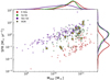 |
Fig. 1. Scatter plot of the relation between SFR versus stellar mass. Galaxies are colour-coded according to their morphological type, and divided into three broad morphological groups as indicated in the legend of the figure. AGN galaxies are marked with golden stars. The normalised distributions of each galaxy population are shown on the top and right sides of the figure. |
3. Method of analysis
There are six main morphological properties that we consider in this study, namely the half-light radius (Rhalf), the Gini and M20 statistics, the concentration (C), the asymmetry (A), and the smoothness (S) parameters. We give a brief definition for each one of these parameters.
The half-light radius is often used to characterise the physical size of a given galaxy. It is defined as the elliptical aperture of the isophote that contains half of the emitted light in a particular wavelength. It has been shown that the size of a galaxy varies with wavelength (e.g. Kelvin et al. 2012; Vulcani et al. 2014; Baes et al. 2020). The change in size may be related to the presence of different stellar or dust components, hence revealing information of the internal structure of galaxies.
Lotz et al. (2004, 2008a) measured the Gini–M20 statistics and introduced a new method to segregate galaxies according to their morphological type and merging status. The Gini coefficient is a quantity traditionally used in economics to measure wealth inequality. However, Abraham et al. (2003) introduced the Gini coefficient and applied it to galaxy images. The Gini index indicates the spread in the pixel values within a predefined aperture. In other words, the Gini index provides an estimate of the concentration of light in the brightest pixels in galaxies with an arbitrary shape. The Gini index is defined as:
 (1)
(1)
where  is the mean flux over the pixel values, fi is the flux of the ith pixel, and k is the total number of pixels assigned to a galaxy. First, the k pixel values are sorted from minimum to maximum. Then, the pixels are divided equally into 50% bright and 50% faint values. When the Gini index is calculated for the bright (faint) pixels it takes positive (negative) values. The final value of the Gini index is calculated by summing up the difference between the brightest and faintest pixels, the second brightest and second faintest pixels, etc, and by dividing the sum by
  . The final range of the Gini index is between 0 and 1. When Gini = 0 then a galaxy has a uniform flux distribution. Conversely, Gini = 1 if the light of the galaxy is concentrated in just few pixels.
Similarly, M20 is another measure of concentration in galaxies, but it is more sensitive to the brightest regions outside the centre of the galaxy. In particular, M20 represents the logarithm of the second moment of the brightest 20% of a galaxy relative to the total second-order central moment, Mtot. The Mtot is calculated through:
![Mathematical equation: $$ \begin{aligned} {M}_{\rm tot} = \sum _{i=1}^{k} {M}_i = \sum _{i=1}^{k} f_i \left[\left(x_i-x_c\right)^2+\left({ y}_i-{ y}_c\right)^2\right], \end{aligned} $$](/articles/aa/full_html/2023/05/aa45962-23/aa45962-23-eq4.gif) (2)
(2)
where fi is the flux of pixel (xi, yi) and (xc, yc) are the coordinates of the galaxy’s centre. M20 is given then by:
 (3)
(3)
where ftot is the total flux of the pixels.
In general, M20 is a suitable parameter to infer the structural properties of galaxies such as spiral arms, bars, rings, tidal perturbations, and multiple nuclei (Lotz et al. 2004; Holwerda et al. 2014).
The CAS system can be used to quantify consistently and objectively the morphological parameters of galaxies. Conselice (2003) argued that the CAS system has the potential of being used as an alternate classification scheme for galaxies, one that is more tightly connected to the physical properties. As its name suggests, the concentration index measures the concentration of the light distribution in galaxies. It is defined as:
 (4)
(4)
with R20 and R80 being the elliptical radii of the isophotes that contain 20% and 80% of the light, respectively. A reasonable correlation has already been found for the concentration of the light distribution with Hubble stage (Morgan 1958, 1959; Okamura et al. 1984; Bershady et al. 2000), bulge-to-disk ratio (Conselice 2003), and supermassive black hole mass (Aswathy & Ravikumar 2018).
The asymmetry index is simply measured by subtracting the galaxy image frame, rotated by 180°, from the original image.
 (5)
(5)
where Abgr is the mean asymmetry value of the background, fij are the pixel fluxes of the original image, and  are the pixel fluxes of the rotated image.
It has been shown that the asymmetry index of star-forming galaxies at optical wavelengths correlates reasonably well with optical broad-band colour (Conselice et al. 2000; Conselice 2003). However, the primary use of this indicator is tracing galaxy mergers and interactions, which often cause strong asymmetries.
Lastly, the smoothness index is obtained by subtracting a smoothed version of the galaxy image frame from the original image. A boxcar of a certain width (0.25 the Petrosian radius) is used to smooth the galaxy’s original image (Lotz et al. 2004). Smoothness is defined as:
 (6)
(6)
where Sbgr is the mean smoothness of the background, fij are the pixel fluxes of the original image, and  are the pixel fluxes of the smoothed image.
Galaxies that have large smoothness values have a more clumpy appearance. That is why the smoothness index is also referred to as the clumpiness index. In principal, this indicator is ideal to segregate between quiescent early-type galaxies and actively star-forming late-type galaxies. Yet, the smoothness index is weakly correlated with SFR (Conselice 2003).
We use the python package StatMorph (Rodriguez-Gomez et al. 2019) to measure the morphological statistics of the CALIFA galaxies. StatMorph was build upon the previous studies by Lotz et al. (2004, 2006, 2008a,b) for calculating the Gini–M20 statistics, and the CAS system indices (Conselice et al. 2000) of a given image. Specifically, we apply StatMorph on each frame included in a CALIFA IFS data cube to retrieve the aforementioned morphological parameters. Of course, the IFU frames contain information on various nebular emission lines as well as absorption features by the stellar continuum. We are interested in measuring if there is a change in morphological structure for different nebular emission lines, and compare with the morphology of the stellar continuum.
In order to retrieve the morphological parameters of emission lines it is imperative to subtract the stellar continuum and integrate the frames belonging to each emission line. Zibetti et al. (2017) provided data cubes with the maps of 25 continuum-subtracted emission lines. To decouple the emission lines from the stellar continuum, the data cubes were preprocessed with an adaptive-kernel smoothing algorithm (see Zibetti 2009; Zibetti et al. 2009, 2017, for more details). The standard pPXF+GANDALF fitting procedure (Cappellari & Emsellem 2004; Sarzi et al. 2006) was then applied to the smoothed cubes. We note that the adaptive smoothing applied to the CALIFA cubes results in a degradation of the spatial resolution at low surface brightness. However, for the adopted detection threshold in this work, the smoothing does not result in a substantial loss of resolution relative to the native PSF of the CALIFA data cubes in most of the cases. In our analysis, we take into account the corresponding noise maps included in the CALIFA IFS and continuum-subtracted emission line data cubes. Figure 2 presents an optical gri broad-band image from SDSS and the individual continuum-subtracted emission line maps of [O III]λ5007, Hα, and [N II]λ6583, of four CALIFA galaxies in our sample. Each galaxy was randomly selected from their corresponding morphological group. It is already evident from this plot that the morphology of the nebular component has some differences with respect to the stellar body of the galaxies.
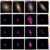 |
Fig. 2. Individual emission-line maps of four galaxies in our sample. Each galaxy was randomly selected from its corresponding morphological group. We also show an AGN host galaxy (fourth column). For each galaxy, we show an optical image from SDSS (top row), and the continuum-subtracted emission-line maps of [O III]λ5007, Hα, and [N II]λ6583. The emission-line maps are in units of normalised flux density. |
For each galaxy we created a segmentation map (Lotz et al. 2004) based on a frame that traces the stellar continuum emission with a detection threshold of 1-σ noise level. The segmentation map is later used for the analysis of all wavelength frames (1900 in total), of a particular galaxy. Regarding the individual nebular emission maps, we calculated the morphological statistics for a range of detection thresholds of their corresponding segmentation map (0.50−3.50σ noise level). From those measurements, we estimated the median and the 16th–84th percentile range of the morphological properties. In our analysis, we use the morphological statistics based on the segmentation map with a detection threshold of 2.50. We provide the uncertainties on the non-parametric morphological properties of the nebular emission maps by quoting the calculated 16th–84th percentile range. We also introduce a minimum error of 5% to account for both underlying systematic effects on the production of the continuum subtracted maps and the measurement of the non-parametric indices.
After applying StatMorph to the CALIFA data cubes, we performed a quality check on the results. In StatMorph there is a flagging system. When flag == 0 the measurements can be trusted, while flag == 1 indicates a problematic measurement. Furthermore, if the mean signal-to-noise ratio (S/N) is lower than 2.5, then the measurements cannot be trusted (Lotz et al. 2006). In the case of the main CALIFA data cubes, most of the frames, if not all, pass those two criteria. There are few problematic frames at the wavelength edges of each data cube that fail both criteria, and therefore we exclude those frames from any statistical calculation. Lastly, in the case of the individual emission lines, we excluded 37 galaxies from the statistical analysis in Sects. 4.2 and 5.3, because StatMorph raised a flag == 1. The majority of those 37 galaxies are E–S0a types (27 galaxies), which are expected not to have strong nebular emission lines. Indeed, a closer inspection of the individual emission line maps of the flagged galaxies revealed that most spaxels have a very low S/N (less than 2.5).
4. Results
In this section, we show the trends of galaxy morphological properties with wavelength. However, our main focus lies in the morphology of the nebular component of a galaxy, and how it differs from the morphology measured from the stellar component. We first consider trends in the morphological parameters as function of wavelength (Sect. 4.1). Later on, we explore the M20–Gini relation of the stellar continuum and of various individual spectral features (Sect. 4.2).
4.1. Morphological parameters vs. wavelength
In Fig. 3 we show the spectral dependence of the main six morphological parameters retrieved by applying Statmorph to the CALIFA data cubes. The following quantities are displayed from top to bottom: the ratio between the half-light size measured in each wavelength over the half-light size measured at 5000 Å, the Gini index, M20, concentration (C), asymmetry (A), and smoothness (S). Galaxies are stacked according to their morphological type, and sorted with increasing SFR per galaxy population. The most prominent spectral features are indicated with the vertical solid lines. In Fig. 4 we show the median trends of each morphological index as a function of rest-frame wavelength. We proceed to discuss the results shown in Fig. 3, panel-by-panel.
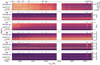 |
Fig. 3. Non-parametric morphological properties as a function of rest-frame wavelength. In this plot we show the results of Statmorph applied on the IFU data of 364 CALIFA galaxies. From top to bottom we present the wavelength dependence of log Rhalf(λ)/Rhalf, 5000 Å, Gini, M20, C, A, and S. The galaxy spectra are stacked according to their morphological type, and they are sorted with increasing SFR per galaxy population. The horizontal dotted lines show the borders between the three galaxy populations. The vertical solid lines indicate the central wavelength of the most prominent spectral features. The white rectangle centred around 5500 Å masks the area of the telluric features in the spectrum. The spectra were binned in wavelength to smooth out the noise. |
ℛ = log Rhalf(λ)/Rhalf, 5000 Å. Instead of displaying the absolute size of galaxies alone, it is often more informative to present the size ratio measured at two different wavelengths. The reasoning is that a ratio such as ℛ can be seen as a conventional colour gradient. We chose to normalise all spectra at 5000 Å due to the flattening of the spectrum beyond that wavelength. Focussing at the top panel of Fig. 3 and the corresponding median trends in Fig. 4, we clearly notice the dependence of galaxy size on wavelength. In all cases, a decreasing gradient can be seen from short to longer wavelengths, in agreement with the results of Kelvin et al. (2012) and Vulcani et al. (2014). All galaxies appear to be more extended (ℛ > 0) at blue wavelengths (< 4500 Å), with their size decreasing as we move towards redder wavelengths, and then remaining roughly constant (> 5000 Å). The change in size with wavelength seems to be more drastic for the late-type galaxies compared to the early types. The observed gradient traces the emission of the various stellar populations. The younger, more extended, stellar disk at shorter wavelengths, and the older, more compact, stellar bulge in the longer wavelengths.
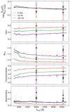 |
Fig. 4. Median trends of the non-parametric morphological properties as a function of rest-frame wavelength. We bin the galaxies according to their morphological type. The coloured markers represent the median values of the non-parametric morphological properties for each galaxy group, as measured from the emission line maps of [O III]λ5007 and Hα. The error bars represent the 16th–84th percentile range. The smoothness index was omitted from this plot due to the small number of wavelength elements with reliable measurement. |
Gini index. In Fig. 3b we show the Gini index as function of wavelength. Qualitatively the Gini index of E–S0a and for many Sa-type galaxies is larger than the Gini index of Sb and Sbc–Sd galaxies. This is the expected behaviour since higher Gini values indicate that the light distribution is concentrated in few pixels, which is true for the early-type galaxies. There is a subtle but non-negligible increasing gradient of Gini with wavelength for Sb and Sbc–Sd galaxies (see also the corresponding median trends in Fig. 4), suggesting that late-type spirals appear less extended at longer optical wavelengths. On average, the Gini index remains roughly constant with wavelength for most galaxies (E–S0a: 0.57; Sa–Sb: 0.53; Sbc–Sd: 0.48).
M20 index. The strongest variation with wavelength is seen for the M20 index in Fig. 3c and middle panel of Fig. 4. Early- and late-type spirals take very large M20 values at the bluest wavelengths (< 4500 Å) followed by a decreasing trend towards redder wavelengths. On the other hand, E–S0a have the lowest values among the different galaxy types and remain roughly constant as a function of wavelength. This means that early-type galaxies are more concentrated across the entire optical wavelength regime, while late-type galaxies are more (less) extended at shorter (longer) wavelengths. In other words, the spiral structure is more prominent at short wavelengths. In addition, Hβ, [O III]λ5007, Hα, and [N II]λ6583 feature prominently in this panel. In late-type galaxies, M20 is always higher for the aforementioned spectral features than for the continuum, regardless of their wavelength range. This is an interesting finding since it is an indication of the differences between the morphology of the stellar continuum and the nebular component of the ISM.
Concentration. The concentration index shares a lot of similarities with both the Gini and M20 statistics. In fact, it has been shown that C anti-correlates with M20 and correlates with Gini (Abraham et al. 2003; Baes et al. 2020). Indeed, in Fig. 3d we notice that for the spiral galaxies C increases with wavelength. Sbc–Sd galaxies are more extended (C < 2.7) at the shortest wavelengths (< 4500 Å), and appear more compact (C > 2.8) with increasing wavelength. E–S0a galaxies are in general more compact with a small relative change in concentration at all optical wavelengths. Similarly to M20, spectral features are visible but they are less pronounced. We note here that M20 is much more sensitive to the morphology of emission lines than the other non-parametric morphological indices.
Asymmetry. In Fig. 3e we illustrate the trends of the asymmetry parameter with wavelength. The asymmetry parameter of each galaxy remains roughly constant across the wavelength range (as it is also seen for the corresponding median trend in Fig. 4). Most, if not all, E–S0a galaxies are more symmetric than the late-type galaxies. This is the expected behaviour as late-type galaxies are actively star-forming, resulting in a very complex internal structure with significant asymmetric features (Hambleton et al. 2011). For spiral galaxies, the emission lines in panel e and in particular Hβ, [O III]λ5007, and Hα display high asymmetry values. Notwithstanding, a lot of the asymmetry signal at the wavelengths corresponding to the most prominent emission lines is due to a kinematic effect caused by the rotation, rather than by structure. The blueshift and redshift that affects the approaching and receding side of the galaxy results in a very strong 180°-asymmetry when looking at individual wavelength frames (i.e. not looking at the emission maps). The flux distribution is only weakly asymmetric once integrate and remove the Doppler shift. In general, the accuracy of the measurement of the A is sensitive to the spatial resolution and S/N (Lotz et al. 2004; Pović et al. 2015). The asymmetry parameter can be reliably measured when S/N > 50. The spatial resolution is crucial too, since objects will appear more symmetric when they are poorly resolved (Conselice et al. 2000).
Smoothness. Smoothness is the least reliable parameter in our analysis. Similarly to asymmetry, the smoothness parameter is prone to noise effects especially for ground-based observations (Lotz et al. 2004; Pović et al. 2015). It also requires a sufficient image resolution (i.e. lower than 1000 pc Lotz et al. 2004), in order to detect if a disk is clumpy or smooth and unfortunately the CALIFA survey does not provide the required spatial resolution (on average 1055 pc). Many of the wavelength elements of the smoothness index return either values very close to zero or values that are entirely unreliable. In the bottom panel of Fig. 3, we only show the smoothness values with a reliable measurement, while we chose to omit the median trends of smoothness from Fig. 4. From the bottom panel of Fig. 3, one can notice that all galaxies appear to be smooth across the wavelength range with Sa galaxies to be more clumpy-like. Interestingly, for the higher S/N dataframes such as the Hα emission line and the surrounding pixels, we are able to detect that the Sb and Sbc–Sd galaxies have more clumpy ISM, since Hα emission originates primarily from star-forming regions. For the rest of the analysis we are not going to discuss S due to the poor image resolution, and because we are using the continuum-subtracted emission line maps which are smoothed with a kernel function, smearing out any resolved clumpy regions.
In Fig. 4, we also show the median values of each galaxy group and for each non-parametric morphological index, as measured from the emission line maps of [O III]λ5007 and Hα. We immediately notice the significant differences between the morphology of the ionised ISM and the stellar continuum emission. In general, the median values of the emission lines for each morphological property and galaxy group, broadly follow the median trends of the corresponding stellar continuum emission, that is E–S0a galaxies appear to be more concentrated and symmetric than Sbc–Sd galaxies. The median values of Gini, M20, and concentration as measured from the nebular lines imply that the morphology of the ionised ISM is less concentrated than the stellar continuum, while from the asymmetry parameter we notice that the nebular morphology is more asymmetric compared to the one of the stellar body. A more detailed analysis of these results follows in Sects. 4.2 and 5.
Once more, we would like to note here that both A and S suffer from large uncertainties and biases for the reasons discussed above. Hence, the results presented in Figs. 3e,f and the bottom panel of Fig. 4 must be interpreted with caution.
4.2. Non-parametric morphology of individual emission line maps – The M20–Gini relation
In this section we present the non-parametric morphological parameters measured for three of the most prominent spectral features in Fig. 3, namely, the [O III]λ5007, Hα, and [N II]λ6583 emission lines. We are interested comparing the parameters of the individual emission lines with the corresponding morphology, measured from the stellar continuum.
We start by focussing on the relation between the Gini index and M20. For each galaxy we derive the non-parametric indicators of the stellar continuum and its corresponding uncertainties, by calculating the median and the 16th–84th percentile range from the non-parametric morphology spectra.
We remind the reader that we excluded 37 galaxies from the statistical analysis of this subsection, because StatMorph raised a flag == 1. After we exclude the flagged galaxies from our sample, we end up with: 72 E–S0a, 116 Sa–Sb, and 139 Sbc–Sd. Out of these galaxies: 12 host an AGN, 122 are edge-on, and 19 are experiencing a merging event.
We plot the M20–Gini relation in Fig. 5. The M20–Gini relation is primarily used to separate galaxies into early or late-type galaxies, as well as to detect mergers. The solid and dashed black lines in each panel of Fig. 5 were defined by Lotz et al. (2008a) to classify galaxies according to their morphology. Galaxies above the solid black line are considered as merger candidates. The area above the dashed black line is usually occupied by early-type galaxies, whereas late-type galaxies are located in the region below the dashed black line.
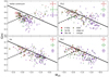 |
Fig. 5. M20–Gini relation for the CALIFA galaxies. Each panel shows the scatter plot of the M20–Gini relation for the stellar continuum and three different spectral features. The solid and dashed black lines are defined in Lotz et al. (2008a). The solid black line roughly separates galaxies between isolated and mergers, whereas the dashed black line divides galaxies into early and late types. Each point represents a galaxy, colour-coded according to their morphological group. AGNs are marked with a golden star. All galaxies with an inclination greater than 80° are marked with a horizontal bar, while all mergers are indicated with a triangle. The average uncertainties of each galaxy group are shown in the top-right corner of each panel. |
According to the morphological parameters measured from the stellar continuum we retrieve a pretty clear separation between E–S0a/Sa–Sb galaxies and Sbc–Sd. Indeed, the more compact objects such as the early types have a more concentrated light distribution (high Gini and low M20 values) than the late-type spiral-galaxies. The 10 out of the 19 classified mergers in our sample fall to the region above the solid black line. We also notice that 24 out of the 122 edge-on galaxies in our sample are located, erroneously, to the same area as the mergers. It has been reported before that edge-on galaxies, as well as bursty galaxies, can contaminate the M20–Gini plane (Bignone et al. 2017). Furthermore, the morphological statistics of AGN galaxies do not show any different characteristics compared to normal galaxies. Therefore, the AGN morphology seems to be determined mainly from the stellar component of their host galaxy. Of course a larger sample of AGNs of different types and with a significant variety of AGN fractions, is required for a proper statistical and morphological analysis.
Looking now at the M20–Gini relation for the individual spectral lines we notice that the Sbc–Sd galaxies appear to be more extended. This means that the nebular and diffuse gas emission is more extended compared to the stellar component. Many of the early-type spiral galaxies, Sa–Sb, now fall bellow the dashed black line and appear to have an equally extended nebular emission as the Sbc–Sd galaxies1. Conversely, E–S0a galaxies remain roughly in the same locus, albeit with increased scatter. Regarding the AGNs, they do not follow any specific trend with the morphology measured from the nebular lines. Furthermore, all nebular lines seem to be in agreement with each other, as expected since their emission originates from the same regions within the galaxies.
Figure 6 illustrates better the change in the M20–Gini plane between the stellar continuum emission and the nebular component. In all three cases, the majority of late-type galaxies are located in the top-left quadrant. Only in the case of [O III], the Sa–Sb galaxies appear to remain as concentrated as their stellar continuum, albeit with an increased scatter. On average, the M20 and Gini index calculated from the nebular emission maps are ∼0.3 dex higher and ∼0.03 dex lower from the corresponding M20 and Gini index of the stellar component. Once again, M20 appears to be more sensitive to the nebular emission. The reason is that M20 traces the brightest regions outside the centre of the galaxy. The larger the value of M20, the further away the brightest pixels are from the centre of the galaxy. In other words, the distribution of the nebular emission in late-type galaxies is more extended than their stellar disk. This effect can contaminate measurements of non-parametric indices based on broad-band images. Contrarily, the nebular component of the E–S0a galaxies, when present, appears to be as compact as the stellar emission.
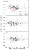 |
Fig. 6. Change in the M20–Gini relation from the stellar to the nebular components. Each point represents a galaxy, colour-coded according to their morphological group. AGNs are marked with a golden star. All galaxies with an inclination greater than 80° are marked with a horizontal bar, while mergers are indicated with a triangle. |
5. Discussion
In this section we discuss the results of our analysis. First, we take a closer look at the wavelength dependence of the physical sizes of galaxies, averaged across various subsets of galaxy populations (Sect. 5.1). Then, we explore how the observed inclination of galaxies affects their measured physical size and concentration index across the optical wavelength range (Sect. 5.2). Last but not least, we consider trends in the morphological parameters with galaxy physical properties, both for the stellar continuum and for individual spectral features (Sect. 5.3).
5.1. Galaxy size vs. wavelength
Over the years, many studies have shown the relation between galaxy size with observed wavelength. La Barbera et al. (2010) showed a 35% decrease in the effective radius of early-type galaxies from optical (g-band) to near-infrared (K-band) wavelengths. Kelvin et al. (2012) extended the study of La Barbera et al. (2010) by including late-type spirals, and found a 25% decrease in their effective radius over the same wavelength range. Vulcani et al. (2014) found that all galaxies regardless of their morphology show a decrease in size towards redder wavelengths. Mosenkov et al. (2019) reported a steady increase in effective radius of the dust with increasing far-infrared wavelengths, highlighting the cold-dust gradient with galactocentric distance. Baes et al. (2020) performed, for the first time, a consistent analysis of the morphological structure of nine late-type DustPedia galaxies (Davies et al. 2017) as a function of wavelength, from ultraviolet (UV) to far-infrared wavelengths. They showed a decrease in galaxy size from UV to NIR, a flattening in the mid-infrared (MIR), and then an increase in the FIR, reaching a comparable size as those measured in the optical bands. In other words, they found that the distribution of interstellar dust in galaxies is as extended as the light distribution by the young stars.
We focus on the dependence of galaxy size with wavelength in the optical regime. But here we present, for the first time, a high spectral resolution, size-wavelength relation for a statistically significant sample of galaxies. The interesting part of this exercise, is that we can eliminate the effects of line emission and isolate the size of the stellar continuum only, something that is not possible when measuring galaxy sizes from broad-band images. We would like to mention again that at any given wavelength, the size Rhalf is defined as the semi-major axis of the elliptical aperture of the isophote containing half the light at that wavelength.
We bin the galaxies into the three main morphological groups, E–S0a, Sa–Sb, and Sbc–Sd. Figure 7 depicts the logarithm of the median trends of Rhalf normalised to Rhalf, 5000 Å as a function of wavelength, and for each galaxy population. All three galaxy populations follow a similar behaviour. At short wavelengths, around 4000 Å, a peak in size is reached. After this peak in size, a decrease follows with increasing wavelength, and beyond 5000 Å the size-wavelength relation becomes flatter.
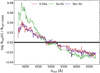 |
Fig. 7. Normalised half-light radius Rhalf as a function of rest-frame wavelength. We bin the galaxies according to their morphological type, and estimate the median spectrum of Rhalf. Then, we normalise with Rhalf, 5000 Å. The spectra were binned in wavelength to smooth out the noise. |
What seems to be related to the morphological type, is the shape of the size-spectrum and the strength of the decrease. Below 5000 Å, Sa–Sb galaxies show the most extreme relative change, since their size decreases steeply about 20% (∼0.08 dex). The decrease in median size both for E–S0a and Sbc–Sd galaxies is smoother. The relative change in median size for the Sbc–Sd group is about 8% (∼0.035 dex), while for the E–S0a is about 10% (∼0.04 dex). Beyond 5000 Å, the size decreases more slowly with increasing wavelength, essentially becoming flat. E–S0a have the slowest change, while Sa–Sb show again the steepest change.
The fact that late-type spirals (Sbc–Sd) have flatter gradients than the early-type spirals (Sa–Sb), provides evidence of the lack of an old bulge in late-type spirals. In other words, it is mainly a central deficit of old stars that make Sbc–Sd galaxies to have a flatter size spectrum with respect to Sa–Sb galaxies. Early-type spirals, instead, have already formed and have largely quiescent bulges, with star formation continuing only in the disk. In addition, the similarity between E–S0a and Sbc–Sd curves indicates a more uniform surface stellar distribution while the change in Sa–Sb galaxies is due to the presence of a more extended bulge.
Another effect that may be responsible for the shape of the size-spectrum and the strength of its decrease is dust attenuation. The effect of dust is stronger in the blue wavelengths, due to the comparable dust grain size with the photon wavelength. Dust particles either absorb or scatter the blue starlight away from the line-of-sight. Therefore, galaxies might appear smaller or larger in size depending on which wavelength regime we are observing at. Lastly, the effects of dust might be stronger depending on the inclination of the system that we observe, as the column density of the dust increases with increasing inclination.
5.2. Inclination effects
In Fig. 7 we presented the existence of a negative gradient between the physical size of galaxies with increasing wavelength. We also noticed that the change is more drastic in some galaxies than others. The explanation is a mix of two effects: the intrinsic age and metallicity gradients of the stellar populations, and dust attenuation at short wavelengths. Yet, the fraction of stellar radiation that is reprocessed by dust, does not only depend upon the inherent properties of dust grains (Draine & Li 2007), but also the geometry of the host galaxy (Gordon et al. 2001; Chevallard et al. 2013). In other words, dust attenuation should be more prominent for the more inclined disk galaxies (e.g. Giovanelli et al. 1994; Battisti et al. 2017; Salim et al. 2018; Yuan et al. 2021; Doore et al. 2021, and references therein).
In order to better understand the variation in size, we explore another dimension in the size-wavelength relation by binning galaxies according to their observed inclination. Moreover, the dust effects are more severe for late-type galaxies than for the early types. In the local Universe, on average, the fraction of bolometric luminosity absorbed by dust in elliptical galaxies is ∼2%, for S0 is ∼9%, for Sa–Sb is ∼25%, while for Sbc-Sd galaxies can range from 23% to 33% (Bianchi et al. 2018; Nersesian et al. 2019). Hence, for this exercise we exclude the ellipticals, as the dust effects in those systems are negligible. We use three bins, separating galaxies into face-on with i ≤ 50° (57 galaxies), edge-on i > 80° (111), and a bin with intermediate inclinations, 50° < i ≤ 80° (144).
Figure 8 shows the median trends of the Rhalf, normalised to the Rhalf, 5000 Å. We also plot size-wavelength relation predicted by Pastrav et al. (2013). That relation was computed for a disk population and by taking into account the effect of dust attenuation. Regarding the edge-on galaxies, their physical size decreases drastically with increasing wavelength, compared to galaxies with low and intermediate inclinations where we see a smoother transition. In particular, there is a decrease of 18% (∼0.07 dex) in size for edge-on galaxies, from 4000 Å to 5000 Å. For the face-on and intermediate inclination galaxies, we see a slower change in size of the order of 11% (∼0.045 dex), at the same wavelength range. The rapid change of the physical size of edge-on galaxies at the shortest wavelengths can be attributed to the increase in optical depth. When observing edge-on galaxies the column density of dust is increasing along the line-of-sight, either absorbing or scattering away the optical starlight.
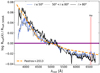 |
Fig. 8. Normalised half-light radius Rhalf as a function of rest-frame wavelength. We bin the galaxies according to their inclination, and estimate the logarithm of the median spectrum of Rhalf. Then, we normalise with Rhalf, 5000 Å. We exclude the elliptical galaxies from this plot, as the effects by dust are negligible. The dashed orange line represents the dependence of size on wavelength for a disk population, and by taking into account the effects of dust. The relation was predicted by Pastrav et al. (2013). The vertical red line indicates the location of the Hα emission line. |
Relative to the Rhalf, 5000 Å, the measured half-light size around ∼4000 Å for the face-on galaxies is smaller by ∼0.03 dex compared to edge-on galaxies. The relative increase in size, from face-on to edge-on, is related to the tracing of the spatial extent of the stellar population, combined with a decrease of light concentration in the central regions of galaxies, where the dust density is higher. Our results are consistent with previous studies (e.g. Möllenhoff et al. 2006; Leslie et al. 2018), who reported an increase in the B-band sizes from face-on to an edge-on disk orientation. At wavelengths beyond 5000 Å, we notice a flattening in Rhalf regardless of the observed inclination.
In some cases, the size of emission lines such as Hα is more extended than the stellar continuum. Primarily, the ionised emission lines originate from H II regions, tracing the ongoing star formation. In Fig. 8 we see that the size of Hα emission in face-on galaxies is increased compared to galaxies of higher inclination, due to the fact that in face-on galaxies we see a larger fraction of the star-forming regions in the disk.
Our results are also in a very good agreement with the predicted trend by Pastrav et al. (2013) for a population of disks affected solely by dust. However, the predicted relation is flatter at longer wavelengths than the observations. Pastrav et al. (2013) found a similar discrepancy when they compared their results with the observed trend by Kelvin et al. (2012). Pastrav et al. (2013) attributed this discrepancy to the intrinsic stellar gradients. Furthermore, Pastrav et al. (2013) have shown that the effects of dust on the structural properties measured in the optical wavelengths, become progressively more severe with increasing inclination. We reach the same conclusion from Fig. 9, where we plot the median trends of the concentration index, as function of wavelength and in inclination bins. We normalise C to the C5000 Å. We find that the concentration of galaxies monotonically increases with wavelength.
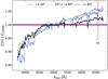 |
Fig. 9. Normalised concentration index C as a function of rest-frame wavelength. We bin the galaxies according to their inclination, and estimate the median spectrum of C. Then we normalise with C5000 Å. Similarly to Fig. 8, we exclude the elliptical galaxies from this plot, as the dust effects are negligible. The vertical red line indicates the location of the Hα emission line. |
At wavelengths between 4000 and 5000 Å, the light distribution of face-on galaxies is less concentrated than edge-on or highly inclined galaxies. In the case of the edge-on galaxies, the change in C at the same wavelength range is more rapid, as they appear more concentrated with increasing wavelength. As the wavelength increases beyond 5000 Å, the concentration index starts to diverge and to take larger values, that is galaxies appear more compact at redder wavelengths. The rate of change in concentration seems to depend on the observed inclination. Overall, we find that the slope becomes steeper with increasing inclination. At wavelengths greater than 5000 Å, the C of edge-on galaxies remains roughly constant, whereas the C of face-on galaxies seems to increase. Lastly, once more we consistently measure that the light distribution of the Hα emission is less concentrated than the stellar continuum, especially evident for the face-on galaxies.
Our analysis confirms that dust effects are increasingly more severe for more highly inclined galaxies. Depending on which wavelength we are observing at, the internal geometry of galaxies can have a significant impact on the measurement of their physical size and morphological properties.
5.3. Non-parametric morphology vs. physical properties
Another interesting topic we want to explore is the relation between morphological indicators and various physical properties, such as SFR, stellar mass, or specific star formation rate (sSFR). The reason is that those physical properties exhibit strong trends with morphology (e.g. Kennicutt 1998; Strateva et al. 2001; Schawinski et al. 2014). In this section we present the best correlation among the physical properties of the CALIFA galaxy sample and the non-parametric properties we measure from the stellar and nebular components. Using a correlation matrix and Pearson’s correlation coefficient (ρ), we quantified the correlations between all of the products in our analysis, and find that the sSFR has the strongest correlations with the concentration index C. The correlation remains moderately strong with C for both the stellar (ρ = −0.47) and nebular emission ([O III]: ρ = −0.50; Hα: ρ = −0.40; [N II]: ρ = −0.47).
The relation between the concentration index and sSFR is illustrated in Fig. 10. From this figure we start to notice differences in the galaxy morphology depending on which spectral feature we are looking at. From the sSFR–C relation of the stellar continuum emission we retrieve a tight correlation with morphology. Galaxies of a certain morphological type reside in a specific location in the sSFR–C plane. Of course, this trend is due to the close correlation between morphological type and sSFR (e.g. Bait et al. 2017; Eales et al. 2017). E–S0a galaxies are populated by an older, more dense and compact stellar population. Their light distribution is concentrated in fewer pixels closer to their nucleus. The intermediate early-type spirals, Sa–Sb galaxies, show a decrease in concentration with increasing sSFR, as they are actively star-forming and therefore having more extended emission than the non-star-forming E–S0a galaxies. Lastly, the late-type spirals, Sbc–Sd, are those with large star-forming disks having the lowest concentration and highest sSFR (high SFR and low stellar mass).
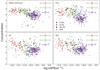 |
Fig. 10. Concentration as a function of sSFR. Each panel shows the scatter plot of the sSFR–C relation for the stellar continuum emission and three spectral lines. Each point represents a galaxy, colour-coded according to the morphological group they are belong to. AGNs are marked with a golden star. The average uncertainties of C for the different galaxy groups are shown in the top-right corner of each panel. We calculate the standard deviation of sSFR for each galaxy population. |
When looking at the same relation measured from the three emission lines we notice a considerable increase in the scatter. However, galaxies still remain well separated according to their morphological group. An interesting point to notice here is that when the C is measured from the stellar continuum it is only possible to separate the E–S0a from the late-type spirals, since both Sa–Sb and Sbc–Sd types have very similar values. A better separation among the morphological types can be achieved when measuring the C from the [O III] emission line.
Moreover, the [O III], Hα, and [N II] show a negative correlation between sSFR and concentration, similar to the continuum emission. Yet again, the nebular emission seems to be less concentrated than the stellar continuum, indicating the extended distribution of the star-forming regions in the disks of galaxies. The concentration of the emission lines in E–S0a is remains roughly constant compared to the stellar continuum. This gives support to the idea that in early-type galaxies any of their remaining ionised gas is mostly concentrated to their central regions.
In Fig. 11 we show the concentration index measured from the stellar continuum and the three most prominent spectral features in the CALIFA data cubes, as a function of sSFR. We separate the data into morphological (left column), mass (middle column), and SFR (right column) bins. We are using the same morphological bins that have been used throughout the paper (excluding the 37 flagged galaxies), as well as a bin that includes all AGNs (12 galaxies) in the sample. For the stellar mass we are using three bins, one of low Mstar (log Mstar < 10.4), moderate Mstar (10.4 ≤ log Mstar < 10.82), and high Mstar (log Mstar ≥ 10.82). Similarly we have three SFR bins, one of low SFR (log SFR < −0.52), moderate SFR (−0.52 ≤ log SFR < 0.14), and high SFR (log SFR ≥ 0.14). All bins were defined in such a way so that they contain roughly one third of the objects in our sample.
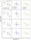 |
Fig. 11. Average trends of the concentration index as a function of sSFR. Each row shows the scatter plot of the sSFR–C relation for the stellar continuum emission and three different spectral lines. Left column: the data are binned according to the morphological group they are belong to, similarly to Fig. 10. Middle column: galaxies are binned according to their stellar mass into low Mstar (log Mstar < 10.4), moderate Mstar (10.4 ≤ log Mstar < 10.82), and high Mstar (log Mstar ≥ 10.82). Right column: galaxies are binned according to their star-formation activity into low SFR (log SFR < −0.52), moderate SFR (−0.52 ≤ log SFR < 0.14), and high SFR (log SFR ≥ 0.14). All bins were defined in such a way so that they contain roughly one third of the objects in our sample. The error bars are the standard deviation of the mean values. |
The left column of Fig. 11 presents the average trends of the scatter plots in Fig. 10. Immediately we notice that C has a decreasing trend with sSFR and that galaxies are clearly separated into early, intermediate, and late types. The same trend can be seen whether we measure the concentration index from the stellar continuum or from the nebular emission lines. On average, early-type galaxies have higher concentration indicating a more compact light distribution. Intermediate galaxies decrease in concentration but overall take similar values as the early types, nevertheless they are less concentrated. The late-type spirals show low concentration and a more extended light distribution, as expected, since they are disk dominated systems.
We find that the mean value of the concentration of early-type galaxies remains roughly constant in all panels. The relative change in C between the stellar continuum and the nebular lines is less than 11%. In late-type galaxies the nebular emission appears to be more extended than the stellar continuum. In particular, for Sa–Sb the mean value of C of the stellar continuum is consistent with the [O III] emission, while the Hα and [N II] emission is less concentrated than the stellar continuum by 15.6% and 6.3%, respectively. For the Sbc–Sd types, we find a difference of 14.3%, 10.7%, and 7% for the [O III], Hα and [N II] emission lines, respectively.
In terms of sSFR, galaxies that host an AGN occupy the same locus as the Sa–Sb types, suggesting that AGNs are in a transitioning phase from actively star-forming to quiescence. This is in agreement with previous studies reporting that AGN galaxies have analogous SFRs with non-AGN galaxies of the same evolutionary stage (Suh et al. 2017; do Nascimento et al. 2019). In AGNs the relative change of the mean C as measured from the stellar continuum and the nebular emission lines is rather small (< 3.3%). Interestingly enough, the C measured from Hα shows a difference from the corresponding value of Sa–Sb galaxies (although the standard deviation is high). On average, it appears that the Hα emission of AGN galaxies is 13% more compact compared to the Sa–Sb galaxies. The most plausible explanation of this result is the extra nuclear emission due to the AGN. Of course, we would like to stress here that the trends we find for AGN have large uncertainties due to the small sample size. Further, investigation with a larger sample is needed to draw robust conclusions.
The middle column of Fig. 11 shows the C as a function of sSFR, binned by stellar mass. We immediately notice that the more massive galaxies are also the more concentrated. Then, the mean C values decrease with increasing sSFR and decreasing stellar mass. By inspecting the right column of Fig. 11 we see that the mean C values decrease as the sSFR increases and the SFR of the galaxies becomes larger. From this we conclude that the more star-forming a galaxy is, the less concentrated it becomes, because star formation is distributed on disks that are generally larger than the pre-existing stellar distribution. The same conclusions can be reached when looking at the mean trends for the nebular emission lines.
In general, we conclude that the apparent morphology of galaxies originates from the starlight distribution, and the morphology of the nebular component differs only moderately from the morphology of the stellar body. Primarily, the emission of the different nebular lines in late-type galaxies probe the light from [H II] regions, tracing the spatial extent of the ongoing star formation in their disk.
5.4. Future applications
The results of this work provide a baseline for more extensive studies both on observational and simulated data. A straightforward application of our methodology could be performed on other integral field spectroscopic surveys such as PHANGS-MUSE (Emsellem et al. 2022) that contains higher spatial resolution, or MaNGA (Bundy et al. 2015) and SAMI (Bryant et al. 2015), that contain larger galaxy samples. Performing a similar analysis, but for a larger statistical sample, will allow for the reported morphological trends in our study to be established further.
Furthermore, our results can be leveraged as benchmark for models of galaxy formation and evolution. The degree to which cosmological hydrodynamical galaxy simulations agree with our results is a major test for them. Specifically, the morphology of galaxies is something that is not considered in the calibration of the models, unlike, for example, the galaxy stellar mass function (e.g. Vogelsberger et al. 2014; Schaye et al. 2015; Pillepich et al. 2018; Davé et al. 2019). Recently, Kapoor et al. (2021) and Camps et al. (2022) provided comparisons of the broadband UV-submm morphological indicators of Auriga (Grand et al. 2017) and ARTEMIS (Font et al. 2020, 2021) simulated galaxies to those from DustPedia observations. In both studies, the authors found that the observed morphological trends as a function of wavelength are in a reasonable agreement with those measured from simulated galaxies. Our work enables for a more detailed comparison of both the stellar continuum and the nebular emission.
6. Summary and conclusions
In this paper, we presented a non-parametric morphology analysis of the stellar continuum and nebular emission lines with a subset of CALIFA galaxies. We explored the dependence of the various morphological parameters on wavelength and morphological type, and quantified the difference in morphology between the stellar and nebular components. The non-parametric morphological indicators were derived with the StatMorph package, applied on the CALIFA IFS data cubes, as well as to the most prominent nebular emission maps, namely [O III]λ5007, Hα, and [N II]λ6583.
We showed a strong gradient, from blue to red optical wavelengths, for the physical size of galaxies, M20 index, and concentration. In particular, we find that M20 is much more sensitive to the morphology of emission lines than the other non-parametric morphological indices. We find that the light distribution of the nebular emission follows the same trend as the stellar continuum, but is less concentrated. From this result we conclude that the apparent morphology of galaxies originates from the stellar light distribution, and that the morphology of the ISM show noticeable differences from the morphology of the stellar component.
A comparison between the non-parametric indicators and the galaxy physical properties, revealed a very strong correlation of the concentration index with the sSFR and morphological type. We find that early-type galaxies are more concentrated than late types. By binning galaxies according to their stellar mass and ongoing SFR, we find that the more massive and low star-forming galaxies are more concentrated, and vice versa.
We also report evidence that the morphology of the nebular emission is more asymmetric and more clumpy than the stellar emission. We note here that the measured values for A and S come with large uncertainties due to the low S/N and spatial resolution of the CALIFA IFS data cubes.
Finally, we explored how galaxy inclination affects our results. We find that high inclined galaxies show a more rapid change in physical size and concentration with increasing optical wavelength, due to the increase in optical depth. Our analysis highlights galaxy inclination as an important aspect of the measurement of the non-parametric morphological indicators, that needs to be considered when interpreting the results.
The median trends of the non-parametric indices as a function of wavelength, for each morphological group, that are shown in Fig. 4, and the Gini, M20, and concentration indices of the stellar continuum and nebular emission lines that were used in the analysis of this work are available in electronic form at the Centre de Données Astronomiques (CDS) de Strasbourg. The morphological parameters as a function of wavelength of each galaxy, presented in Fig. 3, are also available at the CDS.
This is especially true for the Hα and [N II] emission.
Acknowledgments
We would like to thank the referee, Jaime Perea, for the helpful comments and suggestions. A.N. gratefully acknowledges the support of the Research Foundation – Flanders (FWO Vlaanderen). F.D.E. acknowledges funding through the ERC Advanced grant 695671 ‘QUENCH’ and support by the Science and Technology Facilities Council (STFC). This study uses data provided by the Calar Alto Legacy Integral Field Area (CALIFA) survey. Based on observations collected at the Centro Astronómico Hispano Alemán (CAHA) at Calar Alto, operated jointly by the Max-Planck-Institut fűr Astronomie and the Instituto de Astrofísica de Andalucía (CSIC). This research made use of Astropy (http://www.astropy.org), a community-developed core Python package for Astronomy (Astropy Collaboration 2013, 2018).
References
- Abraham, R. G., van den Bergh, S., & Nair, P. 2003, ApJ, 588, 218 [NASA ADS] [CrossRef] [Google Scholar]
- Astropy Collaboration (Robitaille, T. P., et al.) 2013, A&A, 558, A33 [NASA ADS] [CrossRef] [EDP Sciences] [Google Scholar]
- Astropy Collaboration (Price-Whelan, A. M., et al.) 2018, AJ, 156, 123 [Google Scholar]
- Aswathy, S., & Ravikumar, C. D. 2018, MNRAS, 477, 2399 [NASA ADS] [CrossRef] [Google Scholar]
- Baes, M., Nersesian, A., Casasola, V., et al. 2020, A&A, 641, A119 [NASA ADS] [CrossRef] [EDP Sciences] [Google Scholar]
- Bait, O., Barway, S., & Wadadekar, Y. 2017, MNRAS, 471, 2687 [NASA ADS] [CrossRef] [Google Scholar]
- Battisti, A. J., Calzetti, D., & Chary, R. R. 2017, ApJ, 851, 90 [NASA ADS] [CrossRef] [Google Scholar]
- Bershady, M. A., Jangren, A., & Conselice, C. J. 2000, AJ, 119, 2645 [NASA ADS] [CrossRef] [Google Scholar]
- Bianchi, S., De Vis, P., Viaene, S., et al. 2018, A&A, 620, A112 [NASA ADS] [CrossRef] [EDP Sciences] [Google Scholar]
- Bignone, L. A., Tissera, P. B., Sillero, E., et al. 2017, MNRAS, 465, 1106 [NASA ADS] [CrossRef] [Google Scholar]
- Brinchmann, J., Charlot, S., White, S. D. M., et al. 2004, MNRAS, 351, 1151 [Google Scholar]
- Bryant, J. J., Owers, M. S., Robotham, A. S. G., et al. 2015, MNRAS, 447, 2857 [Google Scholar]
- Bundy, K., Bershady, M. A., Law, D. R., et al. 2015, ApJ, 798, 7 [Google Scholar]
- Camps, P., Kapoor, A. U., Trcka, A., et al. 2022, MNRAS, 512, 2728 [NASA ADS] [CrossRef] [Google Scholar]
- Cappellari, M., & Emsellem, E. 2004, PASP, 116, 138 [Google Scholar]
- Cappellari, M., Emsellem, E., Krajnović, D., et al. 2011, MNRAS, 413, 813 [Google Scholar]
- Chevallard, J., Charlot, S., Wandelt, B., & Wild, V. 2013, MNRAS, 432, 2061 [CrossRef] [Google Scholar]
- Conselice, C. J. 2003, ApJS, 147, 1 [NASA ADS] [CrossRef] [Google Scholar]
- Conselice, C. J. 2014, ARA&A, 52, 291 [CrossRef] [Google Scholar]
- Conselice, C. J., Bershady, M. A., & Jangren, A. 2000, ApJ, 529, 886 [NASA ADS] [CrossRef] [Google Scholar]
- Conselice, C. J., Yang, C., & Bluck, A. F. L. 2009, MNRAS, 394, 1956 [NASA ADS] [CrossRef] [Google Scholar]
- Davé, R., Anglés-Alcázar, D., Narayanan, D., et al. 2019, MNRAS, 486, 2827 [Google Scholar]
- Davies, J. I., Baes, M., Bianchi, S., et al. 2017, PASP, 129, 044102 [NASA ADS] [CrossRef] [Google Scholar]
- Davis, T. A., Gensior, J., Bureau, M., et al. 2022, MNRAS, 512, 1522 [CrossRef] [Google Scholar]
- de Vaucouleurs, G. 1959, Handb. Phys., 53, 275 [NASA ADS] [Google Scholar]
- do Nascimento, J. C., Storchi-Bergmann, T., Mallmann, N. D., et al. 2019, MNRAS, 486, 5075 [NASA ADS] [CrossRef] [Google Scholar]
- Doore, K., Eufrasio, R. T., Lehmer, B. D., et al. 2021, ApJ, 923, 26 [NASA ADS] [CrossRef] [Google Scholar]
- Draine, B. T., & Li, A. 2007, ApJ, 657, 810 [CrossRef] [Google Scholar]
- Eales, S., de Vis, P., Smith, M. W. L., et al. 2017, MNRAS, 465, 3125 [NASA ADS] [CrossRef] [Google Scholar]
- Elbaz, D., Daddi, E., Le Borgne, D., et al. 2007, A&A, 468, 33 [NASA ADS] [CrossRef] [EDP Sciences] [Google Scholar]
- Emsellem, E., Schinnerer, E., Santoro, F., et al. 2022, A&A, 659, A191 [NASA ADS] [CrossRef] [EDP Sciences] [Google Scholar]
- Font, A. S., McCarthy, I. G., Poole-Mckenzie, R., et al. 2020, MNRAS, 498, 1765 [NASA ADS] [CrossRef] [Google Scholar]
- Font, A. S., McCarthy, I. G., & Belokurov, V. 2021, MNRAS, 505, 783 [NASA ADS] [CrossRef] [Google Scholar]
- García-Benito, R., Zibetti, S., Sánchez, S. F., et al. 2015, A&A, 576, A135 [Google Scholar]
- Gebek, A., Baes, M., Diemer, B., et al. 2023, MNRAS, 521, 5645 [NASA ADS] [CrossRef] [Google Scholar]
- Giovanelli, R., Haynes, M. P., Salzer, J. J., et al. 1994, AJ, 107, 2036 [NASA ADS] [CrossRef] [Google Scholar]
- Gordon, K. D., Misselt, K. A., Witt, A. N., & Clayton, G. C. 2001, ApJ, 551, 269 [NASA ADS] [CrossRef] [Google Scholar]
- Grand, R. J. J., Gómez, F. A., Marinacci, F., et al. 2017, MNRAS, 467, 179 [NASA ADS] [Google Scholar]
- Hambleton, K. M., Gibson, B. K., Brook, C. B., et al. 2011, MNRAS, 418, 801 [NASA ADS] [CrossRef] [Google Scholar]
- Häußler, B., Bamford, S. P., Vika, M., et al. 2013, MNRAS, 430, 330 [Google Scholar]
- Holwerda, B. W., Pirzkal, N., de Blok, W. J. G., et al. 2011, MNRAS, 416, 2401 [NASA ADS] [CrossRef] [Google Scholar]
- Holwerda, B. W., Muñoz-Mateos, J. C., Comerón, S., et al. 2014, ApJ, 781, 12 [Google Scholar]
- Huertas-Company, M., Tasca, L., Rouan, D., et al. 2009, A&A, 497, 743 [NASA ADS] [CrossRef] [EDP Sciences] [Google Scholar]
- Husemann, B., Jahnke, K., Sánchez, S. F., et al. 2013, A&A, 549, A87 [NASA ADS] [CrossRef] [EDP Sciences] [Google Scholar]
- Kapoor, A. U., Camps, P., Baes, M., et al. 2021, MNRAS, 506, 5703 [NASA ADS] [CrossRef] [Google Scholar]
- Kelvin, L. S., Driver, S. P., Robotham, A. S. G., et al. 2012, MNRAS, 421, 1007 [Google Scholar]
- Kennicutt, R. C., Jr. 1998, ARA&A, 36, 189 [Google Scholar]
- Kewley, L. J., Nicholls, D. C., & Sutherland, R. S. 2019, ARA&A, 57, 511 [Google Scholar]
- La Barbera, F., de Carvalho, R. R., de La Rosa, I. G., et al. 2010, MNRAS, 408, 1313 [CrossRef] [Google Scholar]
- Lacerda, E. A. D., Sánchez, S. F., Cid Fernandes, R., et al. 2020, MNRAS, 492, 3073 [Google Scholar]
- Leslie, S. K., Sargent, M. T., Schinnerer, E., et al. 2018, A&A, 615, A7 [NASA ADS] [CrossRef] [EDP Sciences] [Google Scholar]
- Lintott, C., Schawinski, K., Bamford, S., et al. 2011, MNRAS, 410, 166 [Google Scholar]
- Lotz, J. M., Primack, J., & Madau, P. 2004, AJ, 128, 163 [NASA ADS] [CrossRef] [Google Scholar]
- Lotz, J. M., Madau, P., Giavalisco, M., Primack, J., & Ferguson, H. C. 2006, ApJ, 636, 592 [NASA ADS] [CrossRef] [Google Scholar]
- Lotz, J. M., Davis, M., Faber, S. M., et al. 2008a, ApJ, 672, 177 [NASA ADS] [CrossRef] [Google Scholar]
- Lotz, J. M., Jonsson, P., Cox, T. J., & Primack, J. R. 2008b, MNRAS, 391, 1137 [Google Scholar]
- Möllenhoff, C., Popescu, C. C., & Tuffs, R. J. 2006, A&A, 456, 941 [NASA ADS] [CrossRef] [EDP Sciences] [Google Scholar]
- Morgan, W. W. 1958, PASP, 70, 364 [NASA ADS] [CrossRef] [Google Scholar]
- Morgan, W. W. 1959, PASP, 71, 394 [NASA ADS] [CrossRef] [Google Scholar]
- Mosenkov, A. V., Baes, M., Bianchi, S., et al. 2019, A&A, 622, A132 [NASA ADS] [CrossRef] [EDP Sciences] [Google Scholar]
- Muñoz-Mateos, J. C., Gil de Paz, A., Zamorano, J., et al. 2009, ApJ, 703, 1569 [CrossRef] [Google Scholar]
- Mullaney, J. R., Alexander, D. M., Aird, J., et al. 2015, MNRAS, 453, L83 [Google Scholar]
- Nersesian, A., Xilouris, E. M., Bianchi, S., et al. 2019, A&A, 624, A80 [NASA ADS] [CrossRef] [EDP Sciences] [Google Scholar]
- Noeske, K. G., Weiner, B. J., Faber, S. M., et al. 2007, ApJ, 660, L43 [CrossRef] [Google Scholar]
- Okamura, S., Kodaira, K., & Watanabe, M. 1984, ApJ, 280, 7 [NASA ADS] [CrossRef] [Google Scholar]
- Pastrav, B. A., Popescu, C. C., Tuffs, R. J., & Sansom, A. E. 2013, A&A, 553, A80 [NASA ADS] [CrossRef] [EDP Sciences] [Google Scholar]
- Peng, Y.-J., Lilly, S. J., Kovač, K., et al. 2010, ApJ, 721, 193 [Google Scholar]
- Pillepich, A., Springel, V., Nelson, D., et al. 2018, MNRAS, 473, 4077 [Google Scholar]
- Pović, M., Márquez, I., Masegosa, J., et al. 2015, MNRAS, 453, 1644 [Google Scholar]
- Psychogyios, A., Charmandaris, V., Diaz-Santos, T., et al. 2016, A&A, 591, A1 [NASA ADS] [CrossRef] [EDP Sciences] [Google Scholar]
- Rodriguez-Gomez, V., Snyder, G. F., Lotz, J. M., et al. 2019, MNRAS, 483, 4140 [NASA ADS] [CrossRef] [Google Scholar]
- Salim, S., Boquien, M., & Lee, J. C. 2018, ApJ, 859, 11 [Google Scholar]
- Salpeter, E. E. 1955, ApJ, 121, 161 [Google Scholar]
- Sánchez, S. F., Kennicutt, R. C., Gil de Paz, A., et al. 2012, A&A, 538, A8 [Google Scholar]
- Sánchez, S. F., García-Benito, R., Zibetti, S., et al. 2016, A&A, 594, A36 [Google Scholar]
- Sánchez, S. F., Barrera-Ballesteros, J. K., Sánchez-Menguiano, L., et al. 2017, MNRAS, 469, 2121 [CrossRef] [Google Scholar]
- Sánchez, S. F., Avila-Reese, V., Hernandez-Toledo, H., et al. 2018, Rev. Mex. Astron. Astrofis., 54, 217 [Google Scholar]
- Sandage, A. 2005, ARA&A, 43, 581 [NASA ADS] [CrossRef] [Google Scholar]
- Sarzi, M., Falcón-Barroso, J., Davies, R. L., et al. 2006, MNRAS, 366, 1151 [Google Scholar]
- Schawinski, K., Urry, C. M., Simmons, B. D., et al. 2014, MNRAS, 440, 889 [Google Scholar]
- Schaye, J., Crain, R. A., Bower, R. G., et al. 2015, MNRAS, 446, 521 [Google Scholar]
- Sérsic, J. L. 1963, Boletin de la Asociacion Argentina de Astronomia La Plata Argentina, 6, 41 [Google Scholar]
- Silverman, J. D., Mainieri, V., Lehmer, B. D., et al. 2008, ApJ, 675, 1025 [NASA ADS] [CrossRef] [Google Scholar]
- Simard, L., Mendel, J. T., Patton, D. R., Ellison, S. L., & McConnachie, A. W. 2011, ApJS, 196, 11 [CrossRef] [Google Scholar]
- Speagle, J. S., Steinhardt, C. L., Capak, P. L., & Silverman, J. D. 2014, ApJS, 214, 15 [Google Scholar]
- Strateva, I., Ivezić, Ž., Knapp, G. R., et al. 2001, AJ, 122, 1861 [CrossRef] [Google Scholar]
- Suh, H., Civano, F., Hasinger, G., et al. 2017, ApJ, 841, 102 [NASA ADS] [CrossRef] [Google Scholar]
- Tomczak, A. R., Quadri, R. F., Tran, K.-V. H., et al. 2016, ApJ, 817, 118 [Google Scholar]
- Vogelsberger, M., Genel, S., Springel, V., et al. 2014, Nature, 509, 177 [Google Scholar]
- Vulcani, B., Bamford, S. P., Häußler, B., et al. 2014, MNRAS, 441, 1340 [NASA ADS] [CrossRef] [Google Scholar]
- Walcher, C. J., Wisotzki, L., Bekeraité, S., et al. 2014, A&A, 569, A1 [NASA ADS] [CrossRef] [EDP Sciences] [Google Scholar]
- Whitaker, K. E., van Dokkum, P. G., Brammer, G., & Franx, M. 2012, ApJ, 754, L29 [Google Scholar]
- Yuan, F.-T., Lu, J., Shen, S., & Boquien, M. 2021, ApJ, 911, 145 [NASA ADS] [CrossRef] [Google Scholar]
- Zibetti, S. 2009, ArXiv e-prints [arXiv:0911.4956] [Google Scholar]
- Zibetti, S., Charlot, S., & Rix, H.-W. 2009, MNRAS, 400, 1181 [NASA ADS] [CrossRef] [Google Scholar]
- Zibetti, S., Gallazzi, A. R., Ascasibar, Y., et al. 2017, MNRAS, 468, 1902 [NASA ADS] [Google Scholar]
All Figures
|
Fig. 1. Scatter plot of the relation between SFR versus stellar mass. Galaxies are colour-coded according to their morphological type, and divided into three broad morphological groups as indicated in the legend of the figure. AGN galaxies are marked with golden stars. The normalised distributions of each galaxy population are shown on the top and right sides of the figure. |
| In the text | |
|
Fig. 2. Individual emission-line maps of four galaxies in our sample. Each galaxy was randomly selected from its corresponding morphological group. We also show an AGN host galaxy (fourth column). For each galaxy, we show an optical image from SDSS (top row), and the continuum-subtracted emission-line maps of [O III]λ5007, Hα, and [N II]λ6583. The emission-line maps are in units of normalised flux density. |
| In the text | |
|
Fig. 3. Non-parametric morphological properties as a function of rest-frame wavelength. In this plot we show the results of Statmorph applied on the IFU data of 364 CALIFA galaxies. From top to bottom we present the wavelength dependence of log Rhalf(λ)/Rhalf, 5000 Å, Gini, M20, C, A, and S. The galaxy spectra are stacked according to their morphological type, and they are sorted with increasing SFR per galaxy population. The horizontal dotted lines show the borders between the three galaxy populations. The vertical solid lines indicate the central wavelength of the most prominent spectral features. The white rectangle centred around 5500 Å masks the area of the telluric features in the spectrum. The spectra were binned in wavelength to smooth out the noise. |
| In the text | |
|
Fig. 4. Median trends of the non-parametric morphological properties as a function of rest-frame wavelength. We bin the galaxies according to their morphological type. The coloured markers represent the median values of the non-parametric morphological properties for each galaxy group, as measured from the emission line maps of [O III]λ5007 and Hα. The error bars represent the 16th–84th percentile range. The smoothness index was omitted from this plot due to the small number of wavelength elements with reliable measurement. |
| In the text | |
|
Fig. 5. M20–Gini relation for the CALIFA galaxies. Each panel shows the scatter plot of the M20–Gini relation for the stellar continuum and three different spectral features. The solid and dashed black lines are defined in Lotz et al. (2008a). The solid black line roughly separates galaxies between isolated and mergers, whereas the dashed black line divides galaxies into early and late types. Each point represents a galaxy, colour-coded according to their morphological group. AGNs are marked with a golden star. All galaxies with an inclination greater than 80° are marked with a horizontal bar, while all mergers are indicated with a triangle. The average uncertainties of each galaxy group are shown in the top-right corner of each panel. |
| In the text | |
|
Fig. 6. Change in the M20–Gini relation from the stellar to the nebular components. Each point represents a galaxy, colour-coded according to their morphological group. AGNs are marked with a golden star. All galaxies with an inclination greater than 80° are marked with a horizontal bar, while mergers are indicated with a triangle. |
| In the text | |
|
Fig. 7. Normalised half-light radius Rhalf as a function of rest-frame wavelength. We bin the galaxies according to their morphological type, and estimate the median spectrum of Rhalf. Then, we normalise with Rhalf, 5000 Å. The spectra were binned in wavelength to smooth out the noise. |
| In the text | |
|
Fig. 8. Normalised half-light radius Rhalf as a function of rest-frame wavelength. We bin the galaxies according to their inclination, and estimate the logarithm of the median spectrum of Rhalf. Then, we normalise with Rhalf, 5000 Å. We exclude the elliptical galaxies from this plot, as the effects by dust are negligible. The dashed orange line represents the dependence of size on wavelength for a disk population, and by taking into account the effects of dust. The relation was predicted by Pastrav et al. (2013). The vertical red line indicates the location of the Hα emission line. |
| In the text | |
|
Fig. 9. Normalised concentration index C as a function of rest-frame wavelength. We bin the galaxies according to their inclination, and estimate the median spectrum of C. Then we normalise with C5000 Å. Similarly to Fig. 8, we exclude the elliptical galaxies from this plot, as the dust effects are negligible. The vertical red line indicates the location of the Hα emission line. |
| In the text | |
|
Fig. 10. Concentration as a function of sSFR. Each panel shows the scatter plot of the sSFR–C relation for the stellar continuum emission and three spectral lines. Each point represents a galaxy, colour-coded according to the morphological group they are belong to. AGNs are marked with a golden star. The average uncertainties of C for the different galaxy groups are shown in the top-right corner of each panel. We calculate the standard deviation of sSFR for each galaxy population. |
| In the text | |
|
Fig. 11. Average trends of the concentration index as a function of sSFR. Each row shows the scatter plot of the sSFR–C relation for the stellar continuum emission and three different spectral lines. Left column: the data are binned according to the morphological group they are belong to, similarly to Fig. 10. Middle column: galaxies are binned according to their stellar mass into low Mstar (log Mstar < 10.4), moderate Mstar (10.4 ≤ log Mstar < 10.82), and high Mstar (log Mstar ≥ 10.82). Right column: galaxies are binned according to their star-formation activity into low SFR (log SFR < −0.52), moderate SFR (−0.52 ≤ log SFR < 0.14), and high SFR (log SFR ≥ 0.14). All bins were defined in such a way so that they contain roughly one third of the objects in our sample. The error bars are the standard deviation of the mean values. |
| In the text | |
Current usage metrics show cumulative count of Article Views (full-text article views including HTML views, PDF and ePub downloads, according to the available data) and Abstracts Views on Vision4Press platform.
Data correspond to usage on the plateform after 2015. The current usage metrics is available 48-96 hours after online publication and is updated daily on week days.
Initial download of the metrics may take a while.