| Issue |
A&A
Volume 673, May 2023
|
|
|---|---|---|
| Article Number | A85 | |
| Number of page(s) | 12 | |
| Section | Extragalactic astronomy | |
| DOI | https://doi.org/10.1051/0004-6361/202345936 | |
| Published online | 10 May 2023 | |
Long-term Swift and Metsähovi monitoring of SDSS J164100.10+345452.7 reveals multi-wavelength correlated variability
1
INAF, Osservatorio Astronomico di Brera, Via Emilio Bianchi 46, 23807 Merate (LC), Italy
e-mail: This email address is being protected from spambots. You need JavaScript enabled to view it.
2
Aalto University Metsähovi Radio Observatory, Metsähovintie 114, 02540 Kylmälä, Finland
3
Aalto University Department of Electronics and Nanoengineering, PO Box 15500 00076 Aalto, Finland
4
European Southern Observatory (ESO), Alonso de Córdova 3107, Casilla 19, Santiago 19001, Chile
5
INAF, Osservatorio Astrofisico di Torino, Via Osservatorio 20, 10025 Pino Torinese (TO), Italy
6
Department of Physics, Institute for Astrophysics and Computational Sciences, The Catholic University of America, Washington, DC 20064, USA
7
Dipartimento di Fisica, Università di Trento, Via Sommarive 14, Trento 38123, Italy
8
Dipartimento di Fisica e Astronomia, Università di Padova, 35122 Padova, Italy
9
European Space Agency, European Space Astronomy Centre, C/ Bajo el Castillo s/n, 28692 Villanueva de la Cañada, Madrid, Spain
10
Homer L. Dodge Department of Physics and Astronomy, The University of Oklahoma, 440 W. Brooks St., Norman, OK 73019, USA
11
Università degli Studi di Milano, Bicocca, Piazza delle Scienze 3, 20126 Milano, Italy
Received:
18
January
2023
Accepted:
8
March
2023
Abstract
We report on the first multi-wavelength Swift monitoring campaign performed on SDSS J164100.10+345452.7, a nearby narrow-line Seyfert 1 galaxy that had formerly been considered to be radio-quiet. It has, however, more recently been detected both in the radio (at 37 GHz) and in the γ-ray, a behaviour that hints at the presence of a relativistic jet. During our 20-month Swift campaign, while pursuing the primary goal of assessing the baseline optical/UV and X-ray properties of SDSS J164100.10+345452.7, we observed two radio flaring episodes, namely, one each year. Our strictly simultaneous multi-wavelength data closely match the radio flare and allow us to unambiguously link the jetted radio emission of SDSS J164100.10+345452.7. Indeed, for the X-ray spectra preceding and following the radio flare, a simple absorbed power-law model does not offer an adequate description and, thus, an extra absorption component is required. The average spectrum of SDSS J164100.10+345452.7 can best be described by an absorbed power-law model with a photon index Γ = 1.93 ± 0.12, modified by a partially covering neutral absorber with a covering fraction of f = 0.91−0.03+0.02. On the contrary, the X-ray spectrum closest to the radio flare does not require any such extra absorber and it is much harder (Γflare ∼ 0.7 ± 0.4), thus implying the emergence of an additional, harder spectral component. We interpret this as the jet emission emerging from a gap in the absorber. The fractional variability we derived in the optical/UV and X-ray bands is found to be lower than the typical values reported in the literature because our observations of SDSS J164100.10+345452.7 are dominated by the source being in a low state, as opposed to the literature, where the observations were generally taken as a follow-up of bright flares in other energy bands. Based on the assumption that the origin of the 37 GHz radio flare is the emergence of a jet from an obscuring screen also observed in the X-ray, the derived total jet power is Pjettot = 3.5 × 1042 erg s−1. This result is close to the lowest values measured in the literature.
Key words: galaxies: Seyfert / galaxies: individual: SDSS J164100.10+345452.7 / galaxies: active / X-rays: individuals: SDSS J164100.10+345452.7
© The Authors 2023
 Open Access article, published by EDP Sciences, under the terms of the Creative Commons Attribution License (https://creativecommons.org/licenses/by/4.0), which permits unrestricted use, distribution, and reproduction in any medium, provided the original work is properly cited.
This article is published in open access under the Subscribe to Open model. This email address is being protected from spambots. You need JavaScript enabled to view it. to support open access publication.
1. Introduction
Narrow-line Seyfert 1 galaxies (NLS1s) are active galactic nuclei (AGN) characterised in the optical regime by narrow permitted emission lines (Hβ FWHM < 2000 km s−1, Goodrich 1989), weak forbidden oxygen lines (flux ratio [O III] λ5007/Hβ < 3), and often strong iron emission lines (high Fe II/Hβ, Osterbrock & Pogge 1985). These properties distinguish them from the population of Seyfert 1 galaxies (broad-line Seyfert 1s, BLS1s). Indeed, NLS1s are part of the so-called population A of the AGN main sequence (Sulentic et al. 2002; Sulentic & Marziani 2015; Marziani et al. 2018). In the soft X-ray, NLS1s also have extreme properties, that is, steep spectra (Brandt et al. 1997; Leighly 1999, ΓNLS1 = 2.19 ± 0.10 vs. ΓBLS1 = 1.78 ± 0.11) and fast and large-amplitude variability (Boller et al. 1996), with some showing X-ray flares up to a factor of 100 in flux, on time-scales of days, while BLS1s are generally seen to vary by a factor of a few. These distinctive properties (e.g., Peterson et al. 2004) are customarily understood in terms of low-mass (106–108 M⊙) central black holes and higher accretion rates, close to the Eddington limit (but see, Viswanath et al. 2019). Hence, these are sources that are possibly in an early stage of evolution (Mathur 2000). A small fraction of NLS1s (4–7%, Komossa et al. 2006; Cracco et al. 2016) have been found to be radio-loud1 (Sradio/Soptical > 10) and show a flat radio spectrum (Oshlack et al. 2001; Zhou et al. 2003; Yuan et al. 2008; see also, Lähteenmäki et al. 2017). Additionally, some show a hard spectral component and hard X-ray spectral variability (Foschini et al. 2009).
The further, smaller subclass of γ-ray emitting NLS1 (γ-NLS1) galaxies was recently added to the picture, as a consequence of their detection at high energies (E > 100 MeV) by Fermi-LAT (PMN J0948+0022, Abdo et al. 2009a,b; Foschini et al. 2010). The γ-NLS1 now include about 35 objects (e.g. Romano et al. 2018; Foschini et al. 2021, 2022) whose properties strongly resemble those of jetted sources (see, e.g. Foschini 2012; Foschini et al. 2015; D’Ammando et al. 2016). The calculated jet power (1042.6–1045.6 erg s−1, Foschini et al. 2015), for instance, is lower than that of flat spectrum radio quasars (FSRQs) and partially overlaps that of BL Lacertae objects (BL Lac). Furthermore, the spectral energy distributions (SEDs) of γ-NLS1 galaxies resemble the typical double-humped one of those of other jetted sources such as FSRQs and BL Lacs, as reported in Abdo et al. (2009a,b) and more recently in Foschini et al. (2010, 2015). In particular, Fig. 1 in Foschini et al. (2010) shows the SED of PMN J0948+0022 as compared to the average SEDs of FSRQs and BL Lacs as well as of those of representative radio galaxies such as NGC 6251, M 87, and Centaurus A. The SED of the prototypical γ-NLS1 PMN J0948+0022 lies between those of high-power FSRQs and low-power BL Lacs, which is not surprising given the value of the jet power reported above. Since the radio luminosity function of γ-NLS1 is a continuation (at low luminosity) of that of FSRQs, it is possible that γ-NLS1 are FSRQs in an early stage of their life cycle (Berton et al. 2016, 2017) and the possible differences in observed host galaxies could be explained by ongoing or recent mergers (e.g., Järvelä et al. 2018; Paliya et al. 2020; Shao et al. 2023, but see Varglund et al. 2022 where only one jetted NLS1 shows signs of interaction).
SDSS J164100.10+345452.7 (Zhou et al. 2006), hereon J1641, is a nearby NLS1 (z = 0.16409 ± 0.00002, Albareti et al. 2017) hosted in a spiral galaxy (Olguín-Iglesias et al. 2020), initially classified as radio-quiet. Lähteenmäki et al. (2018), who observed this source 71 times at 37 GHz with the 13.7 m radio telescope at Aalto University Metsähovi Radio Observatory, reported, however, a double detection of J1641 (detection percentage of 2.8%), with an average flux of S37 GHz, ave = 0.37 Jy, and a maximum flux of 0.46 Jy. Since such detections typically suggest the presence of jets, they also sought J1641 in the Fermi-LAT data and obtained a value of SE > 100 MeV = (12.5 ± 2.18)×10−9 ph cm−2 s−1 (with a maximum-likelihood test statistics TS = 39), making this a radio-emitting γ-NLS1. This detection, combined with the Metsähovi detection of six more radio-silent NLS1s and one more radio-quiet NLS1, puts a severe strain on the belief that so-called radio-quiet or radio-silent NLS1s hosted in spiral galaxies are unable to launch jets. New radio observations at low frequencies suggest that the emission of the jet in these objects is absorbed, possibly via a free-free mechanism (Berton et al. 2020; Järvelä et al. 2021). Therefore, NLS1s may harbour a previously unknown class of relativistic jets that are completely undetectable at low radio frequencies, which is where most observations have been carried out to date. J1641 is now part of the sample of approximately one hundred NLS1s frequently monitored at 37 GHz at Metsähovi (Lähteenmäki et al. 2017).
In this paper, we report on a two-year multi-wavelength (optical, ultra-violet, and X-ray) monitoring of J1641 with the Neil Gehrels Swift Observatory (Gehrels et al. 2004) that was performed in 2019–2021 simultaneously with 37 GHz observations obtained as part of the Metsähovi NLS1 monitoring program. In particular, we focus on a 37 GHz flare observed on 2020-05-24 to 2020-05-26. In Sect. 2, we describe the observations and the data reduction. In Sect. 3, we describe our analysis and present our results, while in Sect. 4, we discuss their implications. We adopt the usual Λ-cold dark matter (Λ-CDM) cosmology (Komatsu et al. 2011) with H0 = 70 km s−1 Mpc−1, Ωm = 0.27, and ΩΛ = 0.73 to facilitate direct comparison with the results in Foschini et al. (2015).
2. Observations and data reduction
2.1. Swift
The Swift data were collected through two yearly monitoring campaigns (Target ID 11395, PI: P. Romano) with a pace of one ∼2–3 ks observation per week from 2019-12-09 to 2020-08-17 (97 ks) and from 2021-01-31 to 2021-07-28 (68 ks) with the X–ray Telescope (XRT, Burrows et al. 2005) and the UV/Optical Telescope (UVOT, Roming et al. 2005, with the “U+B+V+all U” filter setup), for a total exposure of 165 ks (68 observations). The pace is ideal for variability studies, since the collected data make up a regular and casual sampling of the light curve of the source at a resolution over about one week, irrespective of the source flux state. We note that each observation may consist of between one and three snapshots (satellite orbits) that are just a few hours apart.
Additionally, three target of opportunity (ToO) observation campaigns (ObsIDs: 00011395030, −032, −033; 00011395035, −036; 00011395038, −039, −042, −044, −046, and −048) were obtained (PI: P. Romano) in response to a radio detection from Metsähovi on 2020-05-24 (MJD 58993–58995; see Sect. 2.2 below) for a total of 16 ks (11 observations). We note that the observing pace of these ToOs is much denser than that of the monitoring campaigns, so when timing analysis was performed, we distinguished the case of the campaign-only dataset from the full dataset. No ToO observations were obtained after the second set of radio detections recorded in 2021. Tables A.1 and A.2 report the log of the Swift/XRT observations for the first and second year, respectively, and include the observing sequence (ObsID), date (MJD of the middle of the observation), start and end times (UTC) of each observation, and XRT exposure time.
The Swift/XRT data were reduced and analysed by using standard procedures within FTOOLS2 (v6.29b) and the calibration database CALDB3 (v20211105). In particular, the XRT data were processed and filtered with the task XRTPIPELINE (v0.13.6). The XRT light curve was generated in the 0.3–10 keV energy range with one point per observation and one per snapshot. We used SOSTA within XIMAGE and adopted the background measured in an annular region with an inner radius of 80 pixels and an external radius of 120 pixels centred at the source position. The PSF losses and vignetting were corrected for by using the appropriate exposure maps. In case of a non-detection, a 3σ upper limit was calculated by using SOSTA and UPLIMIT within XIMAGE and the background defined above. The XRT 0.3–10 keV light curve, binned at one bin per observation, (corresponding to one point per week during the monitoring campaign and several points per week during the ToOs) is shown in Fig. 1. We note that close to the 2020 radio flare J1641 was observed on 2020-05-25 (MJD 58994, observation 029 for 1.7 ks) and on 2020-05-27 (MJD 58996, observation 030 for ∼350 s). Although these observations did not yield a detection on an individual basis (∼1.1 × 10⁻² counts s−1 at the 2.8σ level, and ∼0.01 counts s−1 at the 1.4σ level, respectively), their combination did, at (1.2 ± 0.4)×10−2 counts s−1, so we used this combination as opposed to two upper limits. On the contrary, we discarded observation 069 due to its low exposure (∼350 s) and no close observations to combine it with. For the spectroscopic analysis of the XRT data, source events were extracted from a circular region with a 20 pixel radius; ancillary response files were generated with the task XRTMKARF to account for different extraction regions, vignetting, and PSF corrections; the spectral redistribution matrices in CALDB were used.
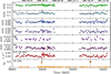 |
Fig. 1. Multi-wavelength light curves of SDSS J164100.10+345452.7. The optical, UV, and X-ray light curves were collected by Swift from 2019-12-09 to 2020-08-17 (first year campaign), from 2021-01-31 to 2021-07-28 (second year), which are shown with 1σ errorbars. The data at 37 GHz were collected at Metsähovi (< 4σ non-detections represented by crosses). Grey bands mark the Metsähovi detections. Top axis reports representative dates during the campaigns. |
The analysis of the UVOT data, which were collected in all filters (optical v, b, u, and UV w1, m2, w2), was performed with the tasks UVOTMAGHIST, UVOTIMSUM, and UVOTSOURCE included in FTOOLS (v6.31 and CALDB v20211108, which offer a check for frames affected by small scale sensitivity, SSS, issues4). UVOTMAGHIST was used to identify the frames of each UVOT image affected by SSS issues and to generate a light curve in each filter at the frame level (the best time resolution available), UVOTIMSUM to sum the sky images for UVOTSOURCE to calculate the magnitude of the source through aperture photometry within a circular region centred on the best source position. This was done by applying the required corrections related to the specific detector characteristics. We adopted circular regions with radii of 5″ and 18″ for the source and background, respectively. We also discarded the source detections that yielded magnitudes with an error > 0.3 mag. The observed light curves (in units of mJy) binned at one point per observation are shown in the six top panels of Fig. 1.
2.2. Metsähovi
The Aalto University Metsähovi Radio Observatory in Finland operates a 13.7 m radio telescope, used for monitoring of AGN at 22 and 37 GHz. The NLS1 monitoring program, fully described in Lähteenmäki et al. (2017), started in 2012 and is currently ongoing. The measurements are carried out with a 1 GHz band dual-beam receiver centred at 36.8 GHz, with typical integration times between 1200 and 1800 s. The detection limit is on the order of 0.2 Jy under optimal conditions. Data points with a signal-to-noise ratio (S/N) of < 4 are handled as non-detections. They may occur either because the source is too faint or because of compromised weather conditions. In the latter case the measurement is discarded. Fainter sources, such as NLS1s, commonly flicker around the detection limit, frequently causing non-detections among the possibly rare detections that occur only when the peak of a flare is seen. The main flux calibrator is DR21, with NGC 7027, 3C 274, and 3C 84 used as secondary calibrators. The full data reduction procedure is reported in Teräsranta et al. (1998).
J1641 is normally observed at least once a week and during more intensive periods, for example, multi-frequency campaigns or flares, even daily. It has now been detected several times since the early reports in Lähteenmäki et al. (2018), with a maximum flux density of 0.65±0.12 Jy on 2019-09-07. In Fig. 1 (bottom panel), we show the data that are simultaneous with the Swift campaigns. Four detections were achieved, on 2020-05-24 (MJD 58993.7820, flux density of 0.38±0.09 Jy), 2020-05-26 (MJD 58995.0987, 0.51±0.11 Jy), 2021-04-07 (MD 59311.9087, 0.49±0.12 Jy), and 2021-04-13 (MJD 59317.8955, 0.48±0.11 Jy). We hereon refer to the May 2020 detections as the 2020 flare, and the April 2021 ones as the 2021 flare. Further detections were obtained after the end of the Swift campaigns on 2021-08-31 (MJD 59457.7556, 0.44±0.09 Jy) and 2021-09-09 (59466.7323, 0.48± 0.09 Jy).
3. Data analysis and results
3.1. Optical, UV, and X-ray variability
As shown in Fig. 1, the Swift light curves show a degree of variability. To quantify it, we computed the fractional variability according to Eqs. (10) and (B2) in Vaughan et al. (2003):
 (1)
(1)
Since the ToO data (after MJD 58996) may introduce a bias towards the high and flaring states, we performed the calculation both over the full dataset ( , ToOs included) and by restricting to the campaign data only (
 ). Table 1 shows the results for both, and, since they are consistent within the errors, from now on, we consider the entire dataset for our analysis. We calculated Fvar from the light curves binned both at the observation and the snapshot levels. Missing values are due to cases where variability was not adequately detected (see Appendix B in Vaughan et al. 2003). We note that the fractional variability measured in J1641 is lower than the typical values reported in D’Ammando (2020) for six well-known γ-ray NLS1s. This is unsurprising, since we focused on a long-term campaign, thus reducing the impact of high flux levels as a consequence of observations triggered by flares observed in other energy bands.
Fractional variability in different energy bands.
The minimum variability time scale in the X-ray energy band is tvar = ln(2) × τd days, where τd is the doubling/halving time defined by:
 (2)
(2)
and F(t1) and F(t2) are the count rates at the times, t1 and t2, respectively. Given that the significance of τd is σ(τd) = |F(t1)−F(t2)|/σ(F(t1)), we selected doubling/halving times with σ(τd)≥3. Table 2 shows the minimum doubling and halving times and their significance when the light curves are binned both at the observation and the snapshot levels. We also note that no difference was found when considering the full dataset or the campaign dataset only. Assuming tvar = ln(2) × (min{τd(R) ; τd(D)}), we find that the minimum variability timescale is  days and
  d or ≃1 h when the light curves are binned at the observation level and at the snapshot level, respectively. In the comoving frame, t′=t (1 + z), we obtained
  days and
 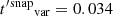 d, respectively.
Doubling and halving times.
The 0.3–10 keV light curve shown in Fig. 1 is characterised by a dynamic range (maximum count rate over minimum count rate) of 3.3. To assess whether this time variability corresponds to detectable spectral variability throughout our monitoring, we calculated the hardness ratio (HR) based on the 0.3–2 keV and 2–10 keV energy bands in the same time binning as the full light curve. We then used it to check for spectral variability on timescales of about one week (the pace of the campaign). We first fit the HR with a constant and obtained (2–10 keV)/(0.3–2 keV) = 0.48 ± 0.02 (χ2 = 83.4, degrees of freedom d.o.f. = 71, null-hypothesis probability nhp = 0.149). We then performed a linear fit that is clearly consistent with the constant fit, since the first-order coefficient is consistent with 0 (χ2 = 82.9, d.o.f. = 70, nhp = 0.138). The F-test probability with respect to the constant is indeed 0.547 (0.6σ). The same procedure was applied to the whole set of observations available on J1641, thus including two archival observations performed on 2019-05-25 and 2019-08-29, along with nine observations we obtained in March 2022 as ToOs. We obtained an F-test probability with respect to the constant of 0.660 (0.95σ), so we can conclude that we did not detect significant spectral variability on timescales of about one week. We note that the same conclusions are reached when the light curve is binned at the snapshot level (few snapshots within a day, separated by about a week) with F-test probabilities below 0.5σ.
3.2. X-ray time-selected spectroscopy
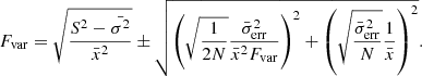
Given the lack of variations in the HR, we first considered two spectra, the one accumulated throughout the whole two-year campaign (‘total’, MJD range 58826–59423, ∼181 ks exposure), and the ‘flare’ spectrum, close to the May 2020 radio flare (MJD 58994–58997, ∼3.5 ks).
We fit the total spectrum with XSPEC (v. 12.12.0, Arnaud 1996) with a simple power-law model (ZPOWERLW, fixed redshift z = 0.16409) corrected for an equivalent hydrogen column corresponding to the Galactic value (fixed 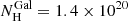 cm−2, HI4PI Collaboration 2016) with the TBABS (Wilms et al. 2000) model. A fit with a neutral absorber in the whole XRT band (0.3–10 keV), yielding a hard photon index Γ = 1.13 ± 0.04, was clearly unacceptable (nhp ∼ 10−26) due to the large negative residuals at energies below 2 keV, suggesting that further absorption was required. This is confirmed by the fact that a fit in the 2–10 keV range yielded reasonable results and a much softer photon index, Γ2 − 10 keV = 1.84 ± 0.15 (see Fig. 2b). The details of the fits are reported in Table 3. To model the excess absorption we added a second absorption component local to the source (ZTBABS) obtaining
 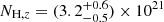 cm−2 and
  (Fig. 2c). The trend in the residuals shown in Fig. 2c, indicates that the model adopted for the extra neutral absorber may not be the most appropriate, so we considered a redshifted absorption edge (ZEDGE). The resulting fit, however, did not reach convergence, with an unphysical edge energy and an unconstrained optical depth, leading to even more prominent residuals below 1 keV. Next, we considered a neutral absorber partially covering the central source, described by a ZPCFABS component, with the redshift of this absorber fixed at the same value as that of the source. This model yielded significant improvement (Δχ2 = −18) over the ZTBABS and, as shown in Fig. 2d, no large-scale structure is left in the data/model ratio. The absorber is characterised by NH, z = (6.2 ± 1.3)×1021 cm−2, a covering fraction
  , while the underlying continuum has a photon index Γ = 1.93 ± 0.12.
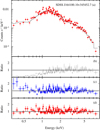 |
Fig. 2. Swift/XRT average spectrum of SDSS J164100.10+345452.7. The data are drawn from the whole two-year observing campaign (details on the spectral fits can be found in Table 3). Panel a: best fit obtained by adopting the model TBABS * ZPCFABS * ZPOWERLW; panel b: data/model ratio from the fit with TBABS * ZPOWERLW in the 2–10 keV band; panel c: data/model ratio from the fit with TBABS * ZTBABS * ZPOWERLW (0.3–10 keV); and panel d: data/model ratio from the fit with TBABS * ZPCFABS * ZPOWERLW (0.3–10 keV). |
Time-selected Swift/XRT spectroscopy.
Finally, we considered the possibility that the absorber is ionised. When using an ABSORI (Done et al. 1992; Magdziarz & Zdziarski 1995; Zdziarski et al. 1995) component, with fixed absorber temperature and Iron abundance, we obtain a significant improvement (Δχ2 = −14) over the ZTBABS model, but a worse fit than the ZPCFABS one. The presence of an ionised absorber partially covering the central source modelled by ZXIPCF is also not supported by the data, since the fit offers no improvement over the ZPCFABS model (see Table 3).
We fit the flare spectrum, consisting of 42 photons, in the 0.3–10 keV band, with the same models as those considered for the total spectrum (see Table 3) by adopting Cash (Cash 1979) statistics. The spectrum can be satisfactorily fit even without an added absorption component. Indeed, for the TBABS * ZTBABS * ZPOWERLW, the TBABS * ZPCFABS * ZPOWERLW and TBABS * ZXIPCF * ZPOWERLW models the NH, z is consistent with zero; for the TBABS * ABSORI * ZPOWERLW model, the fit did not converge, with an ionisation parameter consistent with 0. We note, in particular, that if we fit the flare spectrum with the TBABS * ZTBABS * ZPOWERLW model with the photon index fixed to the mean value (1.75), we obtain 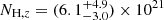 cm−2. This implies that we cannot exclude that extra absorption is indeed present.
We conclude that the total spectrum of J1641 can be best described in the X-ray by an absorbed power-law model modified by a partially covering neutral absorber (TBABS * ZPCFABS * ZPOWERLW), with a covering fraction of  and underlying continuum with a photon index of Γtotal = 1.93 ± 0.12. Conversely, the flare spectrum can be satisfactorily fit even without an added absorption component by adopting a power-law model with a very hard photon index of
 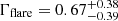 modified just by the Galactic absorption.
Since the XRT data are spread over a 20-month baseline, and guided by the examination of the XRT light curve, we also extracted spectra in several time intervals, as detailed in Table A.3: ‘1st yr’: all observations collected during the first year of the campaign (MJD range 58826–59078, on-source exposure of ∼113.3 ks); ‘2nd yr’: all observations collected during the second year of the campaign (MJD range 59245–59423, ∼67.8 ks); ‘pre0’: all observations preceding the radio flare of 2020-05-24 (MJD range 58826–58987, ∼61 ks); ‘pre1’: close observations preceding the radio flare of 2020-05-24 (MJD 58938–58987, ∼22 ks); ‘plateau’: during an enhanced state of X-ray emission following the radio flare (MJD 59001–59029, ∼23 ks); ‘post’: the remainder of the first year campaign (MJD 59032–59078, ∼24 ks). Since no ToO observations were obtained after the April 2021 radio flare, recorded on 2021-04-07 and 2021-04-13, no XRT data are close enough (≲3 d) to be considered simultaneous; therefore, we did not perform any detailed spectroscopy. We fit all spectra with the same models as those adopted for the total spectrum described above and the results are reported in full in Table A.4. In the case of the TBABS * ZPCFABS * ZPOWERLW model, we note that we obtained consistent covering factors in each time selected spectrum, therefore, we also performed a fit with the covering factor fixed to the value derived from the total spectrum, f = 0.91. In all cases, a simple absorbed power-law model is not an adequate description and an extra absorption component is required.
4. Discussion
We report on the first multi-wavelength Swift monitoring campaign performed on SDSS J164100.10+345452.7, a nearby (z = 0.16409) NLS1 formerly known as radio-quiet which was however recently detected not only in the radio, but also in the γ-rays (Lähteenmäki et al. 2018); this behaviour hints at the presence of a relativistic jet. Our Swift campaign, with a regular pace of one ∼2–3 ks observation per week, lasted two years and was performed with the primary goal of assessing the baseline variability properties (far from radio flares) of J1641 and to obtain matching, multi-wavelength data that are strictly simultaneous with the 37 GHz monitoring data being collected at Metsähovi (Lähteenmäki et al. 2017). Indeed, the campaign covered two distinct radio flaring episodes, one each year and for the first flare (2020-05-24 to 2020-05-26), we also obtained further ToO observations in order to have a denser sampling of the Swift light curves.
4.1. Spectral variability and excess absorption
From our time-selected X-ray spectroscopy (see Table A.4), we find that the source is remarkably stable during the two years of monitoring, with the notable exception of the flare spectrum, extracted almost simultaneously with the radio flare in 2020. The mean spectrum, as represented by the total one in Table 3, is best described by an absorbed power-law model (ZPOWERLW, fixed redshift z = 0.16409), where in addition to the Galactic absorption (TBABS, with fixed  cm−2), an additional absorber is required. We modelled this component with a partially covering (
 ) neutral absorber, (ZPCFABS, see Sect. 3.2). The underlying continuum has a photon index Γtotal = 1.93 ± 0.12, which places J1641 in the bulk of the radio-loud γ-NLS1 population shown in Fig. 2 by Foschini et al. (2015), whose median is Γ = 1.8. Our conclusions stand when considering any of the time selections we performed, particularly those before and after the radio flare.
On the contrary, the X-ray spectrum extracted around the radio flare does not require any absorption in excess of the Galactic one and is much harder, with Γflare ∼ 0.7 ± 0.4. We cannot exclude extra absorption when fitting the flare spectrum with the TBABS * ZTBABS * ZPOWERLW model with the photon index fixed to the mean value (1.75). Indeed, we obtained NH, z < 11 × 1021 cm−2, namely, a value that is considerably higher than that of the mean spectrum. Contrary to the averaged spectrum, in the flare case, the fit shows a hard gamma also when restricted to the hard band, thus suggesting that the source is intrinsically harder. Although it is not unphysical to interpret the simultaneous increase of the X-ray flux and absorption during the flare, we consider it more likely that we are seeing, instead, the presence of a harder spectral component distinct from the softer emission observed out of flare. We can naturally interpret these findings in terms of the jet emission emerging from a gap in the absorber. Consequently, this implies that thanks to the observed correlated radio–X-ray variability, the radio emission during the flare is indeed linked to the presence of a jet in J1641, as opposed to out-of-flare radio emission which may be dominated by star formation activity (Berton et al. 2020), as also testified by the WISE colours W1 − W2 = 1 and W2 − W3 = 4.3 (as derived from NED) which place J1641 outside of the AGN wedge (Mateos et al. 2012, 2013, see also Fig. 3 of Foschini et al. 2015 for a comparison of other radio loud NLS1 and radio loud γ-NLS1s).
We note that we also considered the possibility that the absorber is ionised, in line with the hypothesis put forth by Berton et al. (2020) that the radio emission from the relativistic jet in J1641 can be absorbed in the JVLA bands through free-free absorption due a screen of ionised gas associated with starburst activity (or shocks). And, indeed, an ABSORI component fits the X-ray data reasonably well, although it is not statistically as well as the neutral absorber model. More dedicated optical and X-ray spectral analysis will be presented in a companion paper (Lähteenmäki et al., in prep.) that should help shed light on the nature of the absorber.
4.2. Spectral energy distributions
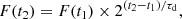
In Fig. 3, we show the radio to γ-ray spectral energy distribution (SED) of J1641, which includes the data obtained during the two-year Swift campaigns, covering the optical/UV + X-ray energy ranges and a representative upper limit from Metsähovi (0.40 Jy), calculated as an average over 15 d, as well as the data obtained during the May 2020 flare (Swift and Metsähovi). We note that this flaring SED is the first strictly simultaneous broad-band SED (radio + optical/UV + X-ray) obtained for this source. The archival SDSS spectrum5 is shown in orange. The grey points, instead, represent historical data drawn from the literature, and they include: JVLA (1.6, 5.2, and 9 GHz, empty triangles, Berton et al. 2020), Metsähovi (37 GHz, filled triangles, Lähteenmäki et al. 2018), and Fermi (filled triangles, Lähteenmäki et al. 2018). We also report data from FIRST, IRAS, WISE, USNO, 2MASS, SDSS, and WGA catalogues, as collected from the ASI/SSDC SED BUILDER TOOL6 (Stratta et al. 2011), which include public catalogues and surveys.
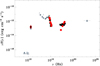 |
Fig. 3. Spectral energy distribution of SDSS J164100.10+345452.7. The black filled square points represent the Swift data obtained during the two-year Swift campaigns; the black filled triangle is a representative Metsähovi upper limit (0.40 Jy) calculated as an average over 15 d, while the red filled circles are the strictly simultaneous ones obtained during the flare of May 2020 (Swift and Metsähovi). The SDSS spectrum is shown in orange. The grey points are drawn from the literature: JVLA 1.6, 5.2, and 9 GHz data (empty triangles), Metsähovi 37 GHz data (filled triangles), and Fermi (filled triangles), as well as FIRST, IRAS, WISE, USNO, 2MASS, SDSS, and WGA catalogues points collected from the ASI/SSDC SED Builder Tool. |
The SED of J1641 resembles those of other jetted sources, with a hint of a double-humped shape. However, we do not have a strictly simultaneous Fermi/LAT detection during the radio flare, therefore it is difficult to constrain the whole SED. We note, however, that the SED of J1641 resemble those of other γ-ray NLS1 galaxies, with a synchrotron peak below  Hz, a host galaxy component peaking at a few ×1014 Hz (as a comparison with a Sb galaxy template indicates), and the X-ray data that could be modelled with a synchrotron self-Compton component (see e.g., Abdo et al. 2009c; Foschini et al. 2015). While the optical-UV data during the May 2020 flare (red points) seem consistent with the average two-year Swift campaigns (black points), the 0.3–10 keV data during the flare have a notably harder spectrum than the average one.
4.3. Energetics
In the following, we compute the quantities related to the physical processes occurring in J1641 and compare them with those of other γ-ray NLS1s. Following the procedure in Berton et al. (2021), we first estimated the luminosity of the Hβ emission line, LHβ = 2.51 × 1041 erg s−1, and used it to calculate the distance of the broad-line region (BLR) from Greene et al. (2010, Table 2),
![Mathematical equation: $$ \begin{aligned} \log \left[ \frac{R_{\rm BLR}}{\mathrm{10\,light\,day}} \right] = 0.85 + 0.53 \log \left[ \frac{L_{\rm H\beta }}{10^{43}\,\mathrm{erg\,s}^{-1}} \right], \end{aligned} $$](/articles/aa/full_html/2023/05/aa45936-23/aa45936-23-eq40.gif) (3)
(3)
which implies RBLR ≃ 2.6 × 1016 cm. The BLR luminosity is calculated according to,
 (4)
(4)
The BLR radiation energy density is then derived from the BLR radius and luminosity,
 (5)
(5)
Given RBLR, we can estimate the accretion disc luminosity (see e.g., Ghisellini & Tavecchio 2009):
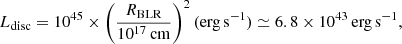 (6)
(6)
which can be normalised to the Eddington luminosity,
 (7)
(7)
assuming MBH = 1.41 × 10⁷ M⊙ as computed in Järvelä et al. (2015). We obtain Ldisc/LEdd ≃ 0.04.
Figure 4 shows the position of J1641 (black filled star) in the Ldisc/LEdd–MBH/M⊙ plane. Open (filled) orange stars mark the place of NLS1 (γ-ray-NLS1) objects, respectively. This plot is adapted from Fig. 4 in Foschini et al. (2015) where red circles are FSRQs and the blue squares are BL Lac objects (blue arrows indicate upper limits in the accretion luminosity). We note that J1641 fits in the region of the γ-ray NLS1 galaxies well.
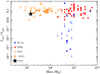 |
Fig. 4. Accretion disc luminosity normalised to the Eddington luminosity as a function of the black-hole mass in solar masses. The black star indicates SDSS J164100.10+345452.7. Symbols and colors are the same as those in Fig. 4 in Foschini et al. (2015). |
Another important quantity that characterises jetted sources is the jet power. Foschini (2014) established two relations between the radiative and kinetic jet power and the luminosity at 15 GHz:
 (8)
(8)
 (9)
(9)
Järvelä et al. (2021) have provided simultaneous radio fluxes at 1.6, 5.2, 9.0 GHz from the Karl G. Jansky Very Large Array (JVLA) and 37 GHz data from the Metsähovi Radio Observatory (non-simultaneous with the JVLA). From these data, we can estimate the radio spectral index7α9.0 − 37 GHz ≃ −4.9, obtaining S15 GHz = 4.3 mJy, when assuming:
 (10)
(10)
with S9.0 GHz = 0.35 mJy and S37 GHz = 370.0 mJy. The K-corrected luminosity equation,
 (11)
(11)
yields L15 GHz = 1.95 × 1040 erg s−1 and allows us to estimate  erg s−1,
  erg s−1, and
 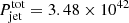 erg s−1. We note that
  erg s−1 is similar to the lowest value in Table 3 of Foschini et al. (2015), corresponding to J0706+3901, whose physical values (see Table 2 in Foschini et al. 2015) are similar to those of J1641. In Table 4, we summarise the results of our calculations.
Overall properties of SDSS J164100.10+345452.7.
5. Summary and conclusions
In this paper we present a 20-month Swift monitoring campaign performed, for the first time, on the newly recognised (Lähteenmäki et al. 2018) γ-NLS1 galaxy SDSS J164100.10+345452.7, which is regularly being observed at the Metsähovi Radio Observatory at the 37 GHz frequency. Our investigation has indeed led us to the following findings and conclusions.
-
We observe minor, but significant variability in the light curves, with an Fvar, as calculated in the UVOT and XRT energy bands, smaller than the values reported in the literature for the best six well-known γ-NLS1s, whose light curves, however, are biased towards flaring states.
-
During the Swift campaign, two radio flares were observed at Metsähovi and, for the first one (May 2020), it was possible to obtain further Swift observations that closely matched the radio ones.
-
From the analysis of the X-ray spectra both preceding and following the radio flare, we find that a simple absorbed power-law model is not adequate and extra absorption is required. Indeed, the average spectrum of J1641 can be best described by an absorbed power-law model with a photon index Γ = 1.93 ± 0.12, modified by a partially covering neutral absorber (covering fraction
 ).
). -
The X-ray spectrum closest to the radio flare, however, does not require extra absorption and is much harder (Γflare ∼ 0.7 ± 0.4). This implies the emergence of an additional, harder spectral component that we interpret as the jet emission peeking out of a gap in the absorber.
-
For this flaring state, we present (also for the first time) a strictly simultaneous SED covering the radio, optical/UV, and X-ray energy bands afforded by the combination of Swift and Metsähovi data. A comparison with the average SED (see Fig. 3) for this object, highlights the harder X-ray spectrum during the radio flare. No obvious variations are observed in the optical, however.
-
Overall, the SED, although it is not well constrained at high energies due to the lack of simultaneous Fermi/LAT data, does show a resemblance to the SEDs of jetted sources, with hints at the presence of two humps. The SED of J1641 is reminiscent of other γ-NLS1 galaxies with a synchrotron peak below 1013 Hz, a host galaxy component peaking at a few 1014 Hz, and the X-ray data which could be modelled with a synchrotron self-Compton component (Abdo et al. 2009c; Foschini et al. 2015).
-
Assuming that the radio emission is due to a jet, we can then calculate its power,
 erg s−1, which is one of the lowest measured when compared with the Foschini et al. (2015) sample, and reminiscent of the γ-NLS1 J0706+3901.
In conclusion, our observations show how a dedicated and well-paced monitoring campaign covering simultaneously the radio (at high frequencies) and the X-ray energy bands can allow us to interpret the source properties observed in different emission states. In particular, in the case of SDSS J164100.10+345452.7, we have been able to detect the ‘smoking-gun’ of the so-called ‘absorbed jet’, originally proposed by Berton et al. (2020). Indeed, the simultaneity and co-spatiality of the radio and X-ray emission show that the nucleus is responsible for the observed flaring of the source. Furthermore, if the origin of the flare were a putative extended emission, detected by JVLA but unresolved by Metsähovi, we would also observe a kpc-scale source with a variability timescale of days, which is not physically possibile. Currently, our knowledge of the absorbed jets is still limited, and only new observations in the X-rays will allow us to confirm if they all show signs of absorption.
We remark that the radio loudness parameter as defined above is becoming more and more inaccurate and unreliable in properly describing these sources, as recently summarised by Berton & Järvelä (2021).
This value needs to be considered with caution as the data are not simultaneous.
Acknowledgments
We thank the anonymous referee for comments that helped to improve the paper. We acknowledge unwavering support from Amos. This work has been partially supported by the ASI-INAF program I/004/11/4. We acknowledge financial contribution from the agreement ASI-INAF n. 2017-14-H.0. This publication makes use of data obtained at Metsähovi Radio Observatory, operated by Aalto University in Finland. We acknowledge the use of public data from the Swift data archive. This research has made use of the NASA/IPAC Extragalactic Database (NED) which is operated by the Jet Propulsion Laboratory, California Institute of Technology, under contract with the National Aeronautics and Space Administration. Part of this work is based on archival data, software or online services provided by the Space Science Data Center – ASI. Happy 18th, Swift.
References
- Abdo, A. A., Ackermann, M., Ajello, M., et al. 2009a, ApJ, 699, 976 [CrossRef] [Google Scholar]
- Abdo, A. A., Ackermann, M., Ajello, M., et al. 2009b, ApJ, 707, 727 [NASA ADS] [CrossRef] [Google Scholar]
- Abdo, A. A., Ackermann, M., Ajello, M., et al. 2009c, ApJ, 707, L142 [NASA ADS] [CrossRef] [Google Scholar]
- Albareti, F. D., Allende Prieto, C., Almeida, A., et al. 2017, ApJS, 233, 25 [Google Scholar]
- Arnaud, K. A. 1996, ASP Conf. Ser., 101, 17 [Google Scholar]
- Berton, M., & Järvelä, E. 2021, Astron. Nachr., 342, 1066 [NASA ADS] [CrossRef] [Google Scholar]
- Berton, M., Caccianiga, A., Foschini, L., et al. 2016, A&A, 591, A98 [NASA ADS] [CrossRef] [EDP Sciences] [Google Scholar]
- Berton, M., Foschini, L., Caccianiga, A., et al. 2017, Front. Astron. Space Sci., 4, 8 [NASA ADS] [CrossRef] [Google Scholar]
- Berton, M., Järvelä, E., Crepaldi, L., et al. 2020, A&A, 636, A64 [NASA ADS] [CrossRef] [EDP Sciences] [Google Scholar]
- Berton, M., Peluso, G., Marziani, P., et al. 2021, A&A, 654, A125 [NASA ADS] [CrossRef] [EDP Sciences] [Google Scholar]
- Boller, T., Brandt, W. N., & Fink, H. 1996, A&A, 305, 53 [NASA ADS] [Google Scholar]
- Brandt, W. N., Mathur, S., & Elvis, M. 1997, MNRAS, 285, L25 [NASA ADS] [CrossRef] [Google Scholar]
- Burrows, D. N., Hill, J. E., Nousek, J. A., et al. 2005, Space Sci. Rev., 120, 165 [Google Scholar]
- Cash, W. 1979, ApJ, 228, 939 [Google Scholar]
- Cracco, V., Ciroi, S., Berton, M., et al. 2016, MNRAS, 462, 1256 [NASA ADS] [CrossRef] [Google Scholar]
- D’Ammando, F. 2020, MNRAS, 496, 2213 [CrossRef] [Google Scholar]
- D’Ammando, F., Orienti, M., Finke, J., et al. 2016, Galaxies, 4, 11 [CrossRef] [Google Scholar]
- Done, C., Mulchaey, J. S., Mushotzky, R. F., & Arnaud, K. A. 1992, ApJ, 395, 275 [NASA ADS] [CrossRef] [Google Scholar]
- Foschini, L. 2012, Proceedings of Nuclei of Seyfert Galaxies and QSOs - Central Engine and Conditions of Star Formation (Seyfert 2012). 6–8 November [Google Scholar]
- Foschini, L. 2014, Int. J. Mod. Phys. Conf. Ser., 28, 1460188P [NASA ADS] [CrossRef] [Google Scholar]
- Foschini, L., Maraschi, L., Tavecchio, F., et al. 2009, Adv. Space Res., 43, 889 [NASA ADS] [CrossRef] [Google Scholar]
- Foschini, L., Fermi/Lat Collaboration, Ghisellini, G., et al. 2010, ASP Conf. Ser., 427, 243 [NASA ADS] [Google Scholar]
- Foschini, L., Berton, M., Caccianiga, A., et al. 2015, A&A, 575, A13 [NASA ADS] [CrossRef] [EDP Sciences] [Google Scholar]
- Foschini, L., Lister, M. L., Antón, S., et al. 2021, Universe, 7, 372 [NASA ADS] [CrossRef] [Google Scholar]
- Foschini, L., Lister, M. L., Andernach, H., et al. 2022, Universe, 8, 587 [NASA ADS] [CrossRef] [Google Scholar]
- Gehrels, N., Chincarini, G., Giommi, P., et al. 2004, ApJ, 611, 1005 [Google Scholar]
- Ghisellini, G., & Tavecchio, F. 2009, MNRAS, 397, 985 [Google Scholar]
- Goodrich, R. W. 1989, ApJ, 342, 224 [Google Scholar]
- Greene, J. E., Hood, C. E., Barth, A. J., et al. 2010, ApJ, 723, 409 [NASA ADS] [CrossRef] [Google Scholar]
- HI4PI Collaboration (Ben Bekhti, N., et al.) 2016, A&A, 594, A116 [NASA ADS] [CrossRef] [EDP Sciences] [Google Scholar]
- Järvelä, E., Lähteenmäki, A., & León-Tavares, J. 2015, A&A, 573, A76 [NASA ADS] [CrossRef] [EDP Sciences] [Google Scholar]
- Järvelä, E., Lähteenmäki, A., & Berton, M. 2018, A&A, 619, A69 [NASA ADS] [CrossRef] [EDP Sciences] [Google Scholar]
- Järvelä, E., Berton, M., & Crepaldi, L. 2021, Front. Astron. Space Sci., 8, 147 [CrossRef] [Google Scholar]
- Komatsu, E., Smith, K. M., Dunkley, J., et al. 2011, ApJS, 192, 18 [Google Scholar]
- Komossa, S., Voges, W., Xu, D., et al. 2006, AJ, 132, 531 [NASA ADS] [CrossRef] [Google Scholar]
- Lähteenmäki, A., Järvelä, E., Hovatta, T., et al. 2017, A&A, 603, A100 [NASA ADS] [CrossRef] [EDP Sciences] [Google Scholar]
- Lähteenmäki, A., Järvelä, E., Ramakrishnan, V., et al. 2018, A&A, 614, L1 [NASA ADS] [CrossRef] [EDP Sciences] [Google Scholar]
- Leighly, K. M. 1999, ApJS, 125, 317 [Google Scholar]
- Magdziarz, P., & Zdziarski, A. A. 1995, MNRAS, 273, 837 [Google Scholar]
- Marziani, P., Dultzin, D., Sulentic, J. W., et al. 2018, Front. Astron. Space Sci., 5, 6 [CrossRef] [Google Scholar]
- Mateos, S., Alonso-Herrero, A., Carrera, F. J., et al. 2012, MNRAS, 426, 3271 [Google Scholar]
- Mateos, S., Alonso-Herrero, A., Carrera, F. J., et al. 2013, MNRAS, 434, 941 [NASA ADS] [CrossRef] [Google Scholar]
- Mathur, S. 2000, MNRAS, 314, L17 [NASA ADS] [CrossRef] [Google Scholar]
- Olguín-Iglesias, A., Kotilainen, J., & Chavushyan, V. 2020, MNRAS, 492, 1450 [Google Scholar]
- Oshlack, A. Y. K. N., Webster, R. L., & Whiting, M. T. 2001, ApJ, 558, 578 [NASA ADS] [CrossRef] [Google Scholar]
- Osterbrock, D. E., & Pogge, R. W. 1985, ApJ, 297, 166 [Google Scholar]
- Paliya, V. S., Pérez, E., García-Benito, R., et al. 2020, ApJ, 892, 133 [CrossRef] [Google Scholar]
- Peterson, B. M., Ferrarese, L., Gilbert, K. M., et al. 2004, ApJ, 613, 682 [Google Scholar]
- Romano, P., Vercellone, S., Foschini, L., et al. 2018, MNRAS, 481, 5046 [NASA ADS] [CrossRef] [Google Scholar]
- Roming, P. W. A., Kennedy, T. E., Mason, K. O., et al. 2005, Space Sci. Rev., 120, 95 [Google Scholar]
- Shao, X., Gu, M., Chen, Y., et al. 2023, ApJ, 943, 136 [NASA ADS] [CrossRef] [Google Scholar]
- Stratta, G., Capalbi, M., Giommi, P., et al. 2011, ArXiv e-prints [arXiv:1103.0749] [Google Scholar]
- Sulentic, J., & Marziani, P. 2015, Front. Astron. Space Sci., 2, 6 [NASA ADS] [CrossRef] [Google Scholar]
- Sulentic, J. W., Marziani, P., Zamanov, R., et al. 2002, ApJ, 566, L71 [NASA ADS] [CrossRef] [Google Scholar]
- Teräsranta, H., Tornikoski, M., Mujunen, A., et al. 1998, A&AS, 132, 305 [NASA ADS] [CrossRef] [EDP Sciences] [Google Scholar]
- Varglund, I., Järvelä, E., Lähteenmäki, A., et al. 2022, A&A, 668, A91 [NASA ADS] [CrossRef] [EDP Sciences] [Google Scholar]
- Vaughan, S., Edelson, R., Warwick, R. S., & Uttley, P. 2003, MNRAS, 345, 1271 [Google Scholar]
- Viswanath, G., Stalin, C. S., Rakshit, S., et al. 2019, ApJ, 881, L24 [NASA ADS] [CrossRef] [Google Scholar]
- Wilms, J., Allen, A., & McCray, R. 2000, ApJ, 542, 914 [Google Scholar]
- Yuan, W., Zhou, H. Y., Komossa, S., et al. 2008, ApJ, 685, 801 [NASA ADS] [CrossRef] [Google Scholar]
- Zdziarski, A. A., Johnson, W. N., Done, C., Smith, D., & McNaron-Brown, K. 1995, ApJ, 438, L63 [NASA ADS] [CrossRef] [Google Scholar]
- Zhou, H.-Y., Wang, T.-G., Dong, X.-B., Zhou, Y.-Y., & Li, C. 2003, ApJ, 584, 147 [NASA ADS] [CrossRef] [Google Scholar]
- Zhou, H., Wang, T., Yuan, W., et al. 2006, ApJS, 166, 128 [NASA ADS] [CrossRef] [Google Scholar]
Appendix A: Supplementary tables and figures
Swift/XRT observation log of SDSS J164100.10+345452.7.
Swift/XRT observation log of SDSS J164100.10+345452.7.
Time-selected Swift/XRT spectroscopy: Time ranges.
Time-selected Swift/XRT spectroscopy: Results.
All Tables
All Figures
|
Fig. 1. Multi-wavelength light curves of SDSS J164100.10+345452.7. The optical, UV, and X-ray light curves were collected by Swift from 2019-12-09 to 2020-08-17 (first year campaign), from 2021-01-31 to 2021-07-28 (second year), which are shown with 1σ errorbars. The data at 37 GHz were collected at Metsähovi (< 4σ non-detections represented by crosses). Grey bands mark the Metsähovi detections. Top axis reports representative dates during the campaigns. |
| In the text | |
|
Fig. 2. Swift/XRT average spectrum of SDSS J164100.10+345452.7. The data are drawn from the whole two-year observing campaign (details on the spectral fits can be found in Table 3). Panel a: best fit obtained by adopting the model TBABS * ZPCFABS * ZPOWERLW; panel b: data/model ratio from the fit with TBABS * ZPOWERLW in the 2–10 keV band; panel c: data/model ratio from the fit with TBABS * ZTBABS * ZPOWERLW (0.3–10 keV); and panel d: data/model ratio from the fit with TBABS * ZPCFABS * ZPOWERLW (0.3–10 keV). |
| In the text | |
|
Fig. 3. Spectral energy distribution of SDSS J164100.10+345452.7. The black filled square points represent the Swift data obtained during the two-year Swift campaigns; the black filled triangle is a representative Metsähovi upper limit (0.40 Jy) calculated as an average over 15 d, while the red filled circles are the strictly simultaneous ones obtained during the flare of May 2020 (Swift and Metsähovi). The SDSS spectrum is shown in orange. The grey points are drawn from the literature: JVLA 1.6, 5.2, and 9 GHz data (empty triangles), Metsähovi 37 GHz data (filled triangles), and Fermi (filled triangles), as well as FIRST, IRAS, WISE, USNO, 2MASS, SDSS, and WGA catalogues points collected from the ASI/SSDC SED Builder Tool. |
| In the text | |
|
Fig. 4. Accretion disc luminosity normalised to the Eddington luminosity as a function of the black-hole mass in solar masses. The black star indicates SDSS J164100.10+345452.7. Symbols and colors are the same as those in Fig. 4 in Foschini et al. (2015). |
| In the text | |
Current usage metrics show cumulative count of Article Views (full-text article views including HTML views, PDF and ePub downloads, according to the available data) and Abstracts Views on Vision4Press platform.
Data correspond to usage on the plateform after 2015. The current usage metrics is available 48-96 hours after online publication and is updated daily on week days.
Initial download of the metrics may take a while.