| Issue |
A&A
Volume 696, April 2025
|
|
|---|---|---|
| Article Number | A74 | |
| Number of page(s) | 22 | |
| Section | Extragalactic astronomy | |
| DOI | https://doi.org/10.1051/0004-6361/202451512 | |
| Published online | 04 April 2025 | |
An optical perspective on early-stage active galactic nuclei with extreme radio flares
1
Dipartimento di Fisica e Astronomia “G. Galilei”, University of Padova, Vicolo dell’osservatorio 3, 35122 Padova, Italy
2
European Southern Observatory, Alonso de Córdova 3107, Casilla 19, 19001 Santiago, Chile
3
INAF – Osservatorio Astronomico di Cagliari, Via della Scienza 5, 09047 Selargius, Italy
4
Departamento de Física y Astronomía, Universidad de La Serena, Av. Cisternas 1200 N, La Serena, Chile
5
Università degli studi dell’Insubria, Via Valleggio 11, 22100 Como, Italy
6
INAF – Osservatorio Astronomico di Brera, Via E. Bianchi 46, 23807 Merate, Italy
7
Laboratory of Instrumentation and Experimental Particle Physics, Av. Prof. Gama Pinto, 2 – 1649-003 Lisboa, Portugal
8
Department of Physics and Astronomy, Texas Tech University, Box 41051 Lubbock, 79409-1051 TX, USA
9
Homer L. Dodge Department of Physics and Astronomy, The University of Oklahoma, 440 West Brooks Street, Norman, 73019 OK, USA
⋆ Corresponding author; This email address is being protected from spambots. You need JavaScript enabled to view it.
Received:
15
July
2024
Accepted:
17
February
2025
Abstract
Over the last decade of active galactic nucleus (AGN) monitoring programs, the Metsähovi Radio Observatory has made multiple detections of seven powerful flaring narrow-line Seyfert 1 (NLS1) galaxies at 37 GHz. Several hypotheses have been proposed, but understanding this unique phenomenon is still far away. To look at the case from a different point of view, we performed an emission line analysis of the optical spectra, with the aim of identifying similarities among the sources, which in turn can possibly be tied with radio behavior. Our data were obtained with the Gran Telescopio Canarias. The results we obtained show that six out of the seven sources have typical properties for the NLS1 class, and one of them is an intermediate Seyfert galaxy. We found on average black hole masses above the median value for the class (> 107 M⊙), and a strong Fe II emission, which could be a proxy for an intense ongoing accretion activity. Although interesting, the characteristics we found are not unusual for this kind of AGN: the optical spectra of our sources do not relate with their unique radio properties. Therefore, further multi-wavelength studies will be necessary to narrow the field of hypotheses for this peculiar phenomenon.
Key words: galaxies: active / galaxies: jets / quasars: emission lines / galaxies: Seyfert
Dodge Family Prize Fellow at The University of Oklahoma.
© The Authors 2025
 Open Access article, published by EDP Sciences, under the terms of the Creative Commons Attribution License (https://creativecommons.org/licenses/by/4.0), which permits unrestricted use, distribution, and reproduction in any medium, provided the original work is properly cited.
This article is published in open access under the Subscribe to Open model. This email address is being protected from spambots. You need JavaScript enabled to view it. to support open access publication.
1. Introduction
Since its classification (Osterbrock & Pogge 1985), the class of active galactic nuclei (AGN) known as narrow-line Seyfert 1 (NLS1) galaxies has been a source of new discoveries. NLS1s have by definition a full width at half maximum (FWHM) of Hβ lower than 2000 km s−1. This limit, even though it is frequently seen in this class, is not strict and it is more a historical convention than a real threshold (Marziani et al. 2018a). Two more criteria, however, clearly distinguish NLS1s: a flux ratio [O III]/Hβ < 3 and prominent Fe II multiplets that are often visible (Cracco et al. 2016; Marziani et al. 2018b, 2021). Moreover, they are characterized by low- to intermediate-mass supermassive black holes (106–108 M⊙), which induce a low rotational velocity of the line-emitting clouds and in turn narrow permitted emission lines (Zhou et al. 2006; Cracco et al. 2016; Chen et al. 2018). Observations suggest an accretion close to or above the Eddington limit (Boroson & Green 1992). As other sources with similar black hole masses, NLS1s belong to population A of the quasar main sequence (Sulentic & Marziani 2015). Their black hole masses lead us to think that they are still in an early phase of their life cycle and that they will eventually evolve, possibly through several accretion episodes, into broad-line Seyfert 1 galaxies (Mathur 2000). Despite the belief that only massive elliptical galaxies are able to launch powerful relativistic jets (Laor 2000), some NLS1s are found to be jetted sources (Abdo et al. 2009a,b; Foschini 2011) that, when face-on, produce γ-ray emission (Foschini et al. 2015). To date ∼70 jetted NLS1s have been confirmed through γ-ray detections (Romano et al. 2018; Paliya et al. 2019) or radio imaging (Richards & Lister 2015; Lister et al. 2016; Berton et al. 2018; Chen et al. 2020, 2022), and several dozen new candidates have been identified (Foschini et al. 2021, 2022). In particular, jetted NLS1s may be an early evolutionary stage of flat-spectrum radio quasars (FSRQs) and the parent population of peaked sources, such as low-luminosity compact sources (Berton et al. 2016a; Foschini 2017; Vietri et al. 2024). The jets in NLS1s are less powerful than those in FSRQs, likely due to the non-linear scaling relations between the jet power and the black hole mass, and the magnetic flux (Heinz & Sunyaev 2003; Foschini et al. 2015; Chamani et al. 2021). These objects are less luminous in radio than FSRQs (Berton et al. 2016a), and they also lack diffuse radio emission (Berton et al. 2018). Hence, because of the lack of relativistic beaming, some jetted NLS1s observed at large angles may actually appear as radio-quiet1.
To increase the number of jetted NLS1s, in 2012 the Metsähovi Radio Observatory (MRO) started a monitoring campaign at 37 GHz (Lähteenmäki et al. 2017). Two of the samples were selected according to completely different criteria, but based on properties that could correlate with their activity in radio. The first includes NLS1s residing in very dense megaparsec-scale environments, such as superclusters (Järvelä et al. 2017); for the second sample sources favorable to a 37 GHz detection were selected, according to their spectral energy distributions (SEDs). Among the two samples, eight sources were detected. In particular, seven of them were detected multiple times, showing flares at jansky-level flux densities (Lähteenmäki et al. 2018) with timescales on the order of days (Järvelä et al. 2024). Such a huge bump in the amplitude was not expected since all of these sources had either weak or no known radio emission before the MRO detections. For one of the sources, Romano et al. (2023) observed an X-ray brightening soon after an MRO detection. Moreover, the same source was identified as a new γ-ray emitter. From the literature, only two sources were detected at 1.4 GHz, at mJy levels, in the Faint Images of the Radio Sky at Twenty-Centimeters survey (FIRST, Becker et al. 1995; Helfand et al. 2015), and the National Radio Astronomy Observatory Very Large Array Sky Survey (NRAO NVSS, Condon et al. 1998).
To untangle the situation, several follow-up radio observations have been carried out. In 2019 the sample was observed with the Karl G. Jansky Very Large Array (JVLA) in A configuration at 1.6, 5.2, and 9.0 GHz (Berton et al. 2020b; Järvelä et al. 2021). Again in 2022, it was observed with the JVLA in A configuration at 10, 15, 22, 33, and 45 GHz and with the Very Long Baseline Array at 15 GHz (Järvelä et al. 2024). In the meantime, single-dish monitoring has been ongoing. In addition to the MRO monitoring, the sources are part of the Owens Valley Radio Observatory 40 m radio telescope AGN monitoring program at 15 GHz (Järvelä et al. 2024). All the data acquired showed steep spectra up to 45 GHz, or no detection at all, especially at high radio frequencies. Although previous cases of such a high-frequency excess are known in the literature (Antonucci & Barvainis 1988), the variability observed, combined with the jansky-level flux densities, are rarely if ever seen in AGN. Because the observations are not simultaneous, the different beam sizes have to be considered, especially comparing single-dish with interferometric observations, with resolved-out structures in the latter. Although a minor difference can be present, resolved-out emission cannot explain such a huge difference in the flux density (Järvelä et al. 2024). Moreover, contamination by close sources has been ruled out (Lähteenmäki et al. 2018; Järvelä et al. 2024). Even though these recent data helped in ruling out some hypotheses, they did not provide a unique and clear answer.
Some viable interpretations for this phenomenon were extensively discussed in Järvelä et al. (2024). One of the possibilities is that these NLS1s could harbor small-scale (likely a few parsecs) relativistic beamed jets, whose low-frequency radio emission is synchrotron self-absorbed or free-free absorbed by ionized gas. The origin of the ionization is unclear, but it could either be due to the abundant star formation often observed in NLS1s (Sani et al. 2010), or to collisions between the jet and the ISM surrounding the AGN, which produces via shocks a cocoon of ionized gas surrounding the jet head (Bicknell et al. 1997). A detailed study of the radio spectral index maps of these sources revealed that the latter is actually the most likely mechanism to account for this unique behavior (Järvelä et al. 2021). Jets-in-jets magnetic reconnection or magnetic reconnection in the black hole magnetosphere are not ruled out either. The latter is particularly interesting since it does not require the presence of relativistic jets.
The implications of this discovery are far-reaching because such large-amplitude variability, coupled with the very short timescales, has never before been observed for this class of sources. This study focuses on the optical spectra of the seven flaring NLS1s, comparing them to each other, and understanding if and how they differ from the spectra of the general NLS1s population. Moreover, we calculated in several ways some of the most important physical parameters for NLS1s such as the broad-line region (BLR) radius, the black hole mass, the Eddington ratio, and the emission lines properties. This paper is organized as follows. In Sect. 2 we introduce the sample. In Sect. 3 we outline the observations performed and the data reduction techniques. In Sect. 4 we describe the emission lines analysis and how we calculated the physical parameters. In Sect. 5 we present our results, and in Sect. 6 we discuss these results. Finally, in Sect. 7 we provide a summary and our conclusions of this work. Throughout this work, we adopt a standard ΛCDM cosmology, with a Hubble constant H0 = 70 km s−1 Mpc−1, and ΩΛ = 0.73 (Komatsu et al. 2011).
2. Sample
As described above, the sample is composed of seven NLS1s detected in a flaring state at 37 GHz by the MRO (Table 1). The sources span a redshift range from 0.0769 to 0.4511. Three out of seven are from the very dense megaparsec-scale environment sample and the remaining four are from the SED-based sample. The radio-loudness parameter has been calculated using the integrated radio fluxes at 5.2 GHz reported in Berton et al. (2020b), and the optical fluxes in the B band. The latter are measured from the optical spectra, using the Johnson-B filter response curve, which is centered at λ0 = 4500 Å with a width of Δλ = 1050 Å. All the sources are radio-quiet (Table 1), even though, as we already described, they present strong flares, which could suggest the presence of relativistic jets. Six sources are hosted in disk-like host galaxies, identified trough a photometric decomposition of their near-infrared images (Järvelä et al. 2018; Olguín-Iglesias et al. 2020; Varglund et al. 2022), and in one case the host galaxy morphology is unknown (for a complete overview on the most recent radio properties of the sample, see Järvelä et al. 2024).
Properties of the sample.
3. Observations and data reduction
The observations were performed with the long-slit spectrometer Optical System for Imaging and low-Intermediate-Resolution Integrated Spectroscopy (OSIRIS) mounted on the Gran Telescopio Canarias (GTC) as part of the program GTC26-22B (P.I. E. Järvelä). The observations were performed using a 0.6 arcsec wide slit, and two different grisms, R1000B and R1000R, to widen the spectral range from 3630 Å to 10 000 Å. The two grisms have a spectral resolution of 1018 and 1122, respectively, and are thus sufficient to sample the main emission lines in the spectra properly. For all the observations, we carried out the standard data reduction using the software Image Reduction and Analysis Facility (IRAF), applying bias and flat-field corrections, and wavelength and flux calibrations. For each source we combined all the single spectra, to maximize the signal-to-noise ratio (S/N), and the final spectra of the two grisms, to obtain the final extended spectrum. However, we were not able to combine the spectra from the two grisms for all sources as in some cases one of the two spectra was too noisy or had bad features, decreasing the quality of the combined spectrum. In those cases, we decided to keep only the best spectrum for the analysis, acquired with either the R1000B or R1000R grism.
We corrected the spectra for galactic absorption using the Cardelli, Clayton, and Mathis extinction law with Rν = 3.1 (Cardelli et al. 1989), which relies on the total extinction parameter, A(V). This parameter is proportional to the column density of neutral hydrogen atoms, NH, by a factor of 5.3 × 10⁻²². We derived NH by means of H I profiles templates2 (Kalberla et al. 2005). The total extinction parameters are shown in Table 2.
Observational parameters derived from the optical spectra.
We tried to apply the host galaxy subtraction by using a technique based on the principal component analysis (La Mura et al. 2007; Chen et al. 2018). However, the shape of the continuum is affected by the combination of the two grisms, and by the contamination of the second spectral order in the R1000R grism. This prevented us from obtaining reliable models of the host spectra. Furthermore, the spectral range covered by only one of the two grisms is also insufficient to perform accurate host modeling. Therefore, we decided to proceed without subtracting the host galaxy. It is worth noting that the host contribution is actually relatively small in sources with z > 0.1 (Letawe et al. 2007), and our analysis mostly focuses on emission lines, which are only marginally affected by the host contribution.
For the iron subtraction, we used the templates available on the Serbian Virtual Observatory3 (Kovačević et al. 2010; Shapovalova et al. 2012). It produces a dedicated iron template with several Fe II lines between 4000 Å and 5500 Å, according to the source’s spectral features. By means of this template we computed the parameter R4570 = F(Fe IIλ4570)/F(Hβ), which is shown in Table 2.
4. Spectral analysis
4.1. Line profiles
To extract the information from the spectra, we fit the line profiles of the main emission lines with several models, using our own python3 code. The S/N of the spectra measured at 5100 Å spans between 12 and 65 (Table 2). We analyzed the most prominent emission lines, such as Hβ, [O III]λλ4959,5007, Hα+[N II]λλ6548,6583, and, when visible, [S II]λλ6716,6731. We measured the spectroscopic redshift using all the forbidden lines present in the spectra, and we double-checked the results with the permitted lines. Even though low-ionization lines are usually less perturbed than high-ionization lines (Komossa et al. 2008), and thus more suitable for redshift measurements, the redshifts we obtained are comparable to those already reported in the literature.
The first lines we modeled were the [O III]λλ4959,5007. Usually in NLS1s the [O III] lines show two main components: a core component produced by the narrow-line region (NLR) gas, which is at the same redshift as the host galaxy, and a wing component, associated with outflowing gas, on the blue side of the line core. Since the outflowing gas clouds can have different velocities, multiple components can be necessary to properly fit their emission profiles. Therefore, we fit each [O III] with two or three Gaussians, one for the core component and one or two for the wing component. To reduce the number of free parameters, we tied certain parameters of the [O III]λ4959 with those of the [O III]λ5007. In particular, we constrained the central position to the rest-frame wavelength and the FWHM, corrected for instrumental resolution, of all the components. Moreover, the flux ratio between the components of the two lines was fixed to the theoretical value of 1/3 (Dimitrijević et al. 2007). Because the spectra are quite noisy, particular attention is needed for a goodness-of-fit test, such as the χ2, in order to deliver reliable results, especially when multiple emission lines are fitted simultaneously. For the [O III] lines we set an interval around the rest-frame position of the two lines in which we computed the χ2, avoiding the non-fitted region between the two lines that would inevitably increase the χ2 value. We calculated these intervals as a multiple of the FWHM of the two [O III] lines, around the central wavelengths of both lines (Fig. 1). Since the outflow emission, when present, is on the blue side of the lines, the bluer side of the interval is often larger compared to the redder side (see Table 2). Finally, exploiting the [O III]λ5007 flux, we measured R5007 = F([O III]λ5007)/F(Hβ) (Table 2).
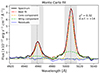 |
Fig. 1. [O III]λλ4959,5007 emission lines of J1641. The light gray shaded regions represent the ranges where the χ2 is assessed. |
To fit Hβ we tried several models for its line profile, with combinations of Gaussian and Lorentzian functions. Overall the best ones turned out to be the two-Gaussian model (2G model), the three-Gaussian model (3G model), and the Lorentzian+Gaussian model (LG model). One of the Gaussians in the 2G and 3G models and the only Gaussian in the LG model represent the narrow component of the Hβ. We constrained their central position to the Hβ rest-frame wavelength and their FWHM, corrected for instrumental resolution, with the FWHM of the [O III]λ5007 core component, leaving the amplitude free to vary. We tied the FWHMs since the narrow component of the Balmer lines is supposed to come from the same region (i.e., the NLR), and thus with the same velocity dispersion as the core component of the forbidden lines. In addition to the narrow component, the remaining Gaussians, one in the 2G model and two in the 3G model, represent the broad emission of Hβ. In the 3G model we had to adopt two Gaussians instead of one, due to the impossibility of properly fitting the wings of the line profile with only one function. In the LG model instead, the broad emission is represented by a Lorentzian function, which is often a good representation of the BLR in NLS1s (Cracco et al. 2016). For the fitting functions of the broad component of Hβ, we calculated the second-order moment, defined as
 (1)
(1)
This parameter was calculated for models built using only Gaussian functions since for a Lorentzian function it is, by definition, equal to infinity.
When visible, we also modeled the [S II]λλ6716,6731 line. We fitted each [S II] profile with a Gaussian function. To reduce the number of free parameters, we constrained the FWHM and the shift, with respect to the rest-frame position, of the Gaussian for [S II]λ6716 with those retrieved with the Gaussian for [S II]λ6731, leaving the flux free to vary.
Finally, we fitted the complex line profile of Hα+[N II]λλ6548,6583, which, as stated before, are blended together. For the Hα line profile, we applied the same model that was used for Hβ (2G, 3G, or LG model), with the same FWHM, corrected for instrumental resolution, and the respective shifts for all the components. For the [N II]λλ6548,6583 we adopted a 2G model in which we constrained the position to the rest-frame wavelength, and the FWHM using [S II] or [O III] width. This is particularly important since the [N II] are completely blended with Hα, and therefore impossible to model without any priors. We preferred [S II] over [O III], when possible, as a reference for [N II] because they are always observed with the same grism and they are both low-ionization lines. We also fixed the flux ratio of the two Gaussians to the value 1/3.049 (Dojčinović et al. 2023). To investigate the internal extinction, we exploited the Balmer decrement calculating the ℛ ratio, defined as the ratio of the Hα to Hβ narrow component fluxes. Following Cardelli et al. (1989), and assuming a theoretical ratio of 2.86, the internal extinction can be expressed as
 (2)
(2)
Once the best-fit model has been selected for all the lines, based on the χ2 and on a visual inspection, we performed a Monte Carlo method, repeating the fit one thousand times. For each iteration we added Gaussian noise to the line profile, proportional to the standard deviation of the signal in the continuum between 5050 Å and 5150 Å. Using a high number of iterations, for each parameter we measured the mean value  and the standard error
  (Ahn & Fessler 2003) defined as
 (3)
(3)
where N is the number of Monte Carlo iterations, Xi the i-th value of the parameter, and σN2 the variance of the parameter expressed as
 (4)
(4)
4.2. Broad-line region radius
We can reasonably assume that the BLR is in a photoionization equilibrium state. The photoionization degree depends on the intensity of the photoionizing radiation, which is proportional to the intensity of all the radiation produced, for AGN, by the accretion flow. Likewise, for the equilibrium assumption, this translates into the intensity of the emission lines produced in the BLR. Furthermore, there is an empirical relation that binds the BLR radius with the luminosity of the accretion disk, such as the 5100 Å continuum, or with the luminosity of emission lines that come from the BLR, such as Hβ. Exploiting Hβ emission, Greene et al. (2010) derived a relation for the BLR radius, expressed as
 (5)
(5)
where L(Hβ) is the integrated luminosity of the line profile, and the BLR radius is expressed in light days. A similar relation was found by Bentz et al. (2013) using the continuum emission at 5100 Å. As mentioned above, the continuum has a small contribution coming from the host galaxy, but we expect it to be inside the flux calibration error, and therefore negligible. Bentz et al. (2013) derived the coefficients of this relation, relying on reverberation mapping data, which is expressed as
 (6)
(6)
with the BLR radius expressed in light days. Recently, an implementation of Eq. (6) for AGN with high Eddington ratios, such as NLS1s, has been derived (Du & Wang 2019; Paliya et al. 2024). Du & Wang (2019) found that the RHβ–L5100 relationship (Kaspi et al. 2000; Bentz et al. 2009, 2013) diverges from the more precise results obtained through the most recent reverberation mapping data. By means of analyzing the sample, they found a strong dependence on Fe IIλ4570 emission, modifying Eq. (6) as
 (7)
(7)
where R4570 is the ratio described in Sect. 3. Therefore, we calculated the BLR radius through Eq. (7) whenever the R4570 was available. Only for one source was the Fe IIλ4570 emission not measurable. In this case we calculated the BLR radius using Eqs. (5) and (6). For all the formulas described we performed an error propagation for the uncertainties estimation. It is important to remember that all the cited equations for the BLR radius calculation were derived empirically from real data. Therefore, they are never free from biases.
4.3. Black hole mass
Assuming virialized gas orbiting the black hole, the virial theorem can be used to express the black hole mass as
 (8)
(8)
where RBLR is the radius of the BLR, ν is the rotational velocity of the gas, G is the gravitational constant, and f is the scaling factor. In Eq. (8), the two main unknowns are the BLR radius and the velocity. These quantities can be derived in many different ways. In the case of the BLR radius, we already described in the previous section the three types of relations that can be used starting from different observables, namely Hβ luminosity (Eq. (5)), 5100 Å continuum luminosity (Eqs. (6) and (7)), and R4570 (Eq. (7)). Two independent parameters can also be used as a proxy for the rotational velocity v. The first is the FWHM of the Hβ broad component. We derived it using the functions in the line fitting process, which modeled only the broad emission of Hβ. In particular, the cited functions were a Gaussian for the 2G model, two Gaussians for the 3G model, and a Lorentzian for the LG model. Alternatively, we adopted the second-order moment (Eq. (1)) as a proxy for v. As mentioned above, we did not calculate such a parameter for the LG model as it is equal to infinity for the Lorentzian function. Several studies emphasize how the second-order moment is more reliable than the FWHM(Hβb) as a proxy for the rotational velocity, being less affected by inclination effects and the BLR geometry (Peterson et al. 2004; Peterson 2011; Peterson & Dalla Bontà 2018). Nevertheless, we decided to use both methods, reducing the probability of systematics and biases that each single assumption can have.
The parameter v represents the rotational velocity of the gas in the BLR, while the FWHM(Hβb) is instead an observable of the velocity dispersion. This difference is included in Eq. (8) by the f factor. The black hole mass formula defined above is a theoretical relation for a completely virialized gas in a perfect Keplerian motion, a case that basically never occurs in AGN. The main sources of uncertainty are the BLR geometry and its inclination. It is clear that the measurable velocities for a flat BLR, seen face-on or edge-on, are different. In the former, the rotational velocity can even be close to zero, leading to an underestimation of the black hole mass (Decarli et al. 2008). However, although not negligible, in NLS1s the inclination effect might be not so significant (Vietri et al. 2018; Berton et al. 2020a) since a significant vertical structure in the BLR can be present (Kollatschny & Zetzl 2011, 2013). On the other hand, a spherical BLR geometry is even harder to handle with just a relatively simple formula. The f factor accounts for the differences between the theoretical formula and the actual black hole mass by correcting the rotational velocity observables. The most recent knowledge shows that a Keplerian motion of the BLR clouds is present (Peterson & Wandel 1999; GRAVITY Collaboration 2018), possibly with additional components such as turbulent vertical motions originating in a disk wind (Gaskell 2009; Kollatschny & Zetzl 2013). Moreover, it has been found that f is inversely proportional to the FWHM(Hβ) (Shen & Ho 2014). Mandal et al. (2021) estimated a typical range for the f factor between 0.8 and 5, mostly derived from a comparison with reverberation mapping observations. For this work we decided to use the f factors estimated by Collin et al. (2006), which are fσ = 3.93 and fFWHM = 2.12 for the rotational velocity obtained by the second-order moment and the FWHM(Hβb), respectively.
Summarizing, when the Hβ profile was modeled by either the 2G or the 3G model, we obtained two different black hole mass estimates, using Eq. (7) for the BLR radius, and considering the ways in which we calculated the v parameter. When we applied the LG model instead, we obtained the two black hole mass estimates using only the FWHM(Hβb) as a proxy for the rotational velocity, and Eqs. (5) and (6) for the BLR radius. In all cases, to retrieve the associated error for each black hole mass we applied a standard error propagation.
4.4. Eddington ratio
For AGN, the Eddington ratio is defined as
 (9)
(9)
where Lbol is the bolometric luminosity, and LEdd is the Eddington luminosity. Objects with high ϵ, even higher than 1, usually show strong Fe II multiplets and narrow Hβ, while low Eddington objects show broader Hβ and a weak Fe II emission. Such differences also translate to a different position in the quasar main sequence (Marziani et al. 2018b). For NLS1s a typical Eddington ratio is between 0.1 and 1 (Boroson & Green 1992; Williams et al. 2002, 2004; Grupe et al. 2010; Xu et al. 2012), but sometimes even super-Eddington accretion has been observed (Chen et al. 2018; Tortosa et al. 2022). The bolometric luminosity can be derived by exploiting simple relations with observables, such as the 5100 Å continuum luminosity formula (Netzer 2019) expressed as
 (10)
(10)
where kbol is the bolometric correction factor defined as
![Mathematical equation: $$ \begin{aligned} k_{\rm bol} = 40 \left[ \frac{\lambda L_\lambda (5100\,{\AA })}{10^{42}~\mathrm {erg\ s}^{-1} } \right]^{-0.2} . \end{aligned} $$](/articles/aa/full_html/2025/04/aa51512-24/aa51512-24-eq13.gif) (11)
(11)
The main uncertainty of kbol comes from the inclination of the AGN accretion disk with respect to the line of sight. Netzer (2019) estimated that for type 1 AGN the bolometric correction factor decreases by a factor of ∼1.4 on average, and by a factor of ∼2.5 for face-on accretion disks. Since the inclination of the analyzed sources is unknown, and consequently to account for all the possible inclinations, we decided to take  as the bolometric correction factor, and
  as its uncertainty. In general, Eqs. (10) and (11) are particularly affected by the jet presence and can be partially affected by the host galaxy contribution, since both of these components can contribute to the continuum luminosity. However, in our case the presence of the jet is still debated, and the host component is only marginal; therefore, we decided to keep such relation to estimate ϵ. Alternatively, we also used an approach less affected by non-nuclear contributions. We retrieved the 5100 Å continuum luminosity for Eqs. (10) and (11) using the Lλ(5100 Å)-L(Hβb) relation (Ilić et al. 2017; Dalla Bontà et al. 2020) defined as
![Mathematical equation: $$ \begin{aligned} \log (\lambda L_\lambda (5100\,{\AA }) )&= (43.396\pm 0.018) + (1.003\pm 0.022) \nonumber \\&\quad \times [\log (L(\mathrm {H}\beta _b)) - 41.746] . \end{aligned} $$](/articles/aa/full_html/2025/04/aa51512-24/aa51512-24-eq16.gif) (12)
(12)
This approach allowed us to indirectly calculate the continuum luminosity, and consequently the bolometric luminosity, exploiting the Hβ properties. Its flux is directly proportional to the ionizing continuum of the AGN, which is free from jet and host contamination. For the Eddington ratio calculation we averaged the black hole mass of each source. Also in this case we applied a proper error propagation for the error calculation through all the described steps.
5. Results
5.1. SDSS J102906.69+555625.2
J1029, with a redshift of 0.4511, is the farthest source in the sample. Due to its distance, the Hα and [S II] region is inside the portion of the spectrum contaminated by the sky emission. Therefore, in this case, we only managed to analyze Hβ and [O III]λλ4959,5007 emission lines. Moreover, due to a bad feature on the bluer part of the spectrum, probably of instrumental origin, we kept only the R1000R grism spectrum. The fitting models we adopted were the 3G model for Hβ and the four-Gaussian model for the [O III]λλ4959,5007 since these last do not show any asymmetric shape. This source, with values of 2132 km s−1 and 2856 km s−1, has the highest FWHM(Hβ) and σ respectively. Its FWHM(Hβb) is 2320 km s−1, which means that it is not formally an NLS1, but it still shares all the properties of Population A sources. Averaging the results in Table 3, it has the highest black hole mass in the sample, equal to (6.63 ± 1.88)×107 M⊙. Such characteristics, coupled with a moderate Eddington ratio of 0.07 on average (Table 3), could be traits of an NLS1 in an evolved stage, possibly transitioning into a classical broad-line AGN.
Black hole mass and Eddington ratio results.
5.2. SDSS J122844.81+501751.2
Also in this case we kept only the R1000R grism spectrum since the R1000B grism spectrum had a much worse S/N, making it difficult to model the continuum. For the emission lines the applied fitting models were the 3G model for Hβ and Hα, and the six-Gaussian model for the [O III]λλ4959,5007. Thanks to a S/N of 65, the highest in the sample, the asymmetric profiles on the two [O III] emission lines are clearly visible (Fig. 2). Therefore, six Gaussian functions were necessary to properly fit these profiles. In NLS1s, classified as high-accretion sources, the [O III] blue wing is associated with powerful outflows that can be generated by the radiation pressure coming from the accretion disk or a jet (Proga et al. 2000; Greene & Ho 2005). The wing components, usually broader than the core component, are likely produced in the innermost part of the NLR (Berton et al. 2016b). In our case the two Gaussians used to model the wing components are shifted by −163 and −371 km s−1 toward the blue side. The average mass of the black hole is (9.21 ± 4.96)×106 M⊙, and the calculated Eddington ratios are 0.94 ± 0.19 and 0.11 ± 0.02. In agreement with these values (see Sect. 6.3 for the discussion), the R4570 is the highest in the sample (2.81), suggesting strong Fe II multiplets emission.
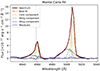 |
Fig. 2. [O III]λλ4959,5007 line profiles of J1228. |
5.3. SDSS J123220.11+495721.8
The emission line parameters for J1232 were derived using the 3G fitting model for the Hβ and Hα lines, and the six-Gaussian model for the [O III]λλ4959,5007. Along the whole spectrum the permitted lines are much stronger than the forbidden lines (Fig. 3). Moreover, the [O III]λλ4959,5007 profile shows core components that are fainter compared to the wing components (Fig. 4). The two Gaussians used to model the blue side of the [O III] lines are shifted about −411 km s−1 and −596 km s−1. According to these, we can classify this source as a blue outlier (Marziani et al. 2003; Komossa et al. 2008; Berton et al. 2016b; Schmidt et al. 2018), following the criterion adopted by Zamanov et al. (2002) ([O III] wing component with a shift < −250 km s−1). The origin of blue outliers could be due to a jet interacting with the NLR as they correlate with the radio emission (Berton et al. 2021), but also due to winds produced by strong radiation pressure-driven outflows in a high-Eddington source (Komossa et al. 2008; Marziani et al. 2016). The latter is likely the case here since this is the source with the second-highest Eddington ratio we found (∼0.27). Also in this case the R4570 = 1.58 suggests strong Fe II multiplets emission, especially considering the high flux of the Hβ (8.14 × 10⁻¹⁵ erg s−1 cm−2), placing J1232 in the A4 population region of the quasar main sequence (Sulentic & Marziani 2015). The mean black hole mass of (2.73 ± 0.88)×107 M⊙ is well inside the range for NLS1s.
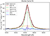 |
Fig. 3. Hα+[N II]λλ6548,6583 line profiles of J1232. The cyan dashed line represents the [N II] line profiles, which are much fainter than the Hα emission. |
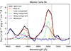 |
Fig. 4. [O III]λλ4959,5007 line profiles of J1232, which show wing components stronger than the core components. |
5.4. SDSS J150916.18+613716.7
For this source we used the 3G model for the fitting of the Hβ and Hα lines, and the six-Gaussian model for the fitting of the [O III]λλ4959,5007 lines. Even thought the six-Gaussian model was necessary to fit the [O III] lines, they did not show strong asymmetric wings. The Hβ line has a FWHM of 1744 km s−1, inside the range for NLS1s. The mean black hole mass we obtained is (3.02 ± 0.73)×107 M⊙ and the Eddington ratio is around 0.06. The R4570 of 1.06 and the Hβ flux of 2.20 × 10⁻¹⁵ erg s−1 cm−2, respectively the lowest and second-highest values in the sample, suggest faint Fe II emission. It is worth noting that the faint iron emission in this case is only in comparison to the other sources in the sample since all the sources for which we manage to measure the R4570 belong to populations A3 and A4 of the quasar main sequence.
5.5. SDSS J151020.06+554722.0
With a black hole mass on average equal to (8.03 ± 3.83)×106 M⊙, J1510 has the second-lowest mass in the sample and an average Eddington ratio of 0.15. The applied fitting models to the spectrum were the 3G model for the Hβ and Hα lines, and the four-Gaussian model for the [O III]λλ4959,5007. Even in this case, the [O III] emission lines are quite symmetric, without strong evidence of outflows. A defect, possibly due to uncontrolled reflections inside the instrument, affected the blue side of the Hβ profile. Therefore, the measured FWHM(Hβ) of 1031 km s−1, although already quite narrow, might have been slightly overestimated, thus causing an overestimation of the black hole mass. The second-order moment of the line, equal to 2307 km s−1, is roughly twice the FWHM(Hβ), which can be explained by the overestimated width of the line.
5.6. SDSS J152205.41+393441.3
J1522 is the closest source, with a redshift of 0.0769. As we did for J1228, we used only the R1000R grism spectrum because in comparison the R1000B grism spectrum had a S/N that was eight to ten times worse. Here the [S II] lines were too faint to be distinguished from the noise; therefore, we used the FWHM of [O III]λ5007 core component as a reference for the FWHM of [N II] lines. The best fitting models turned out to be the four-Gaussian model for the [O III]λλ4959,5007, and the LG model for the Hβ and Hα lines. Since we used a Lorentzian to fit the broad components of the emission lines, we did not calculate the second-order moment for this source. Using only the FWHM(Hβb) as a proxy for the velocity parameter, we obtained the lowest value for the black hole mass of the whole sample, on average equal to (3.14 ± 0.54)×106 M⊙. Considering that J1522 has the second-highest Eddington ratio derived from the measured continuum luminosity at 5100 Å, we could classify it as an NLS1 in an early evolutionary stage. However, the resulting lower ϵ using the derived continuum luminosity, as described in Sect. 4.4, suggests an overestimation of the former Eddington ratio, likely due to contamination by the host galaxy. This hypothesis derives from the vicinity of the source, and from the presence of absorption lines in the spectrum, which can be produced only by the host galaxy. This contamination cannot be estimated since a proper host galaxy modeling was not possible, due to the unusable bluer spectrum.
5.7. SDSS J164100.10+345452.7
J1641 shows peculiar line profiles compared to the rest of the sample. The broad components of the Hβ line, with an FWHM of 4050 km s−1 is the broadest among the analyzed sources. This value, coupled with the FWHM of the narrow component of 493 km s−1 translates to a line profile (Fig. 5) typical for intermediate Seyfert galaxies (Osterbrock 1991; Dalla Barba et al. 2023). To properly fit the Hβ shape we used a 2G model. A four-Gaussian model was used for the [O III]λλ4959,5007 lines. Two Gaussians for each [O III] line were enough to achieve a good fit since no evidence of outflows was present. We did not perform a fitting of the Hα profile since it was strongly contaminated by the sky emission, impossible to remove despite several attempts. According to the results, J1641 turned out to be one of the sources with the lowest Eddington ratio, equal to 0.17 ± 0.04 and 0.01 ± 0.01. This source was found to be the only γ-ray emitter in the sample, hinting at the presence of a relativistic beamed jet (Lähteenmäki et al. 2018). This feature, coupled with the relatively low Eddington ratio and high FWHM(Hβ), might suggest an advanced evolutionary stage (Foschini 2017).
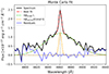 |
Fig. 5. Hβ line profile of J1641. The broad and narrow components have a FWHM of 4050 km s−1 and 493 km s−1, respectively. |
6. Discussion
In this paper we analyzed the optical spectra of seven NLS1s with extreme radio features. We did so by performing a model fitting of the main emission lines. The goal was to investigate for similar characteristics among these sources by comparing their physical properties, such as black hole mass and Eddington ratio, and the emission line profiles.
6.1. Black hole mass
From Table 3, the black hole mass calculated using the second-order moment turned out to be on average larger than that obtained with the FWHM(Hβb). It is due to the fact that the σ we measured is systematically larger than the FWHM(Hβ). This is not uncommon in NLS1s as the values for σ and FWHM(Hβ) can be different from each other, yielding significantly different results (see, e.g., Foschini et al. 2015). The physical meaning of such a discrepancy is not easy to address. The FWHM(Hβb) is, by definition, a directly measurable geometric property of the line, which is the reason why most studies tend to use this simple parameter (see, e.g., the large surveys by Rakshit et al. 2017; Paliya et al. 2024). However, even a small difference in line width drives a large variability in the output (i.e., the black hole mass) because of its quadratic dependence shown in Eq. (8). The way the line width is measured, for instance, the FWHM, has several limitations. This becomes particularly evident when an emission line presents a complex line profile. As described in Sect. 5, in all the cases but two the resulting broad profile in the Hβ line is no longer represented by a single function, but is instead a composition of two functions. However, the measured FWHM comes mostly only from one of the two, according to the amplitude of each component. It leads to an overestimation of the mass when the lines are broader and an underestimation when the lines are narrower (Peterson & Dalla Bontà 2018). This means that two different Hβ lines can yield the same black hole mass estimate in all those cases where the main broad component is described by the same function. On the other hand, the second-order moment is more sensitive to the whole broad profile. This issue has already been widely discussed (Peterson et al. 2004; Peterson 2011), and σ is likely the most reliable proxy for the gas velocity.
In two cases (J1522 and J1641), however, we modeled the Hβ broad component using only one function. According to what we have discussed so far, in these two cases the black hole masses derived with the FWHM(Hβb) and the second-order moment should be comparable. However, for J1522, the broad component in the Hβ line was modeled using a Lorentzian profile; therefore, a comparison between the two methods is literally impossible since the second-order moment of a Lorentzian function cannot be measured. However, since it shows all the typical traits of NLS1s, we believe that the estimated black hole mass calculated with the FWHM of the Lorentzian profile is reliable. J1641, instead, turned out to be an intermediate Seyfert galaxy (Osterbrock & Koski 1976; Osterbrock 1977), and not an NLS1. The same classification can be retrieved by looking at the Sloan Digital Sky Survey (SDSS) spectrum. The main characteristic that distinguishes the two classes is the ratio of the narrow to the broad component, which is much higher in the intermediate Seyfert galaxies. The intermediate Seyfert galaxies are further subdivided according to the prominence of the broad component of the emission lines compared to the narrow component (Dalla Barba et al. 2023). The origin of these objects is widely discussed, spanning from inclination effects to intrinsic processes (Barquín-González et al. 2024). In the inclination hypothesis, the optical features visible in the spectra of intermediate Seyfert galaxies are due to the partial obscuration of the BLR (Malkan et al. 1998; Guainazzi et al. 2005). In this case there would be an underestimation of the real width of the broad components in the emission lines. As a consequence, it can affect the calculation of the black hole mass and the Eddington ratio. In particular, an underestimation of the line width yields an underestimation of the black hole mass, and consequently an overestimation of the Eddington ratio. In our case this means that J1641 may have a more massive black hole than estimated. Considering that J1641 was found to be a γ-ray source, a more massive black hole would strengthen our hypothesis about its advanced stage of evolution.
The results we found in this work are systematically higher than previously estimated (Järvelä et al. 2015). This is most likely due to the fact that past calculations adopted a totally different approach, that led to lower mass values. To further investigate the reliability of the results we obtained with Eq. (8), we additionally measured the black hole masses using a recent scaling law derived by Shen et al. (2024). They derived a relation comparing the masses of single epoch spectra with the values obtained with the reverberation mapping technique, exploiting the Lλ(5100 Å) and the FWHM(Hβ). The black hole masses we measured using such relation are listed in Table A.1. Comparing the results obtained with this scaling law and the virial theorem, we found very similar values, confirming the reliability of the main approach we used. Shen et al. (2024) derived similar scaling laws for the Mg II and C IV emission lines. Nevertheless, these two relations cannot be used in our case since both Mg II and C IV are not visible in the spectra analyzed because of spectral coverage.
On average, the black hole masses derived for the whole sample are well within the typical range of NLS1s population (Peterson 2011). However, almost all of them lie above the median value for the class (MBH = 1 × 10⁷, Cracco et al. 2016), except for J1522. This is in agreement with the typical values in jetted NLS1s. Jetted NLS1s tend to have higher black hole masses than is usually observed in non-jetted NLS1s (Foschini et al. 2015; Berton et al. 2015). Nevertheless, only based on the results obtained in this study, we cannot prove the presence of relativistic jets. It is worth noting, however, that the mass difference observed between jetted and non-jetted sources may be due to an observational bias. Since the power of relativistic jets scales non-linearly with the black hole mass (Heinz & Sunyaev 2003; Foschini 2014), more massive black holes have brighter relativistic jets, which in turn are easier to detect. Therefore, we may still be missing the population of jetted NLS1s of lower mass. J1522 could fall exactly into this population. The Lorentzian profile for the broad Hβ suggests a source in an early stage of evolution (Berton et al. 2020a), indicating that the relatively low black hole mass does not derive from an underestimation.
6.2. Eddington ratio
Regardless of the method used, the Eddington ratio of our sources is also consistent with typical NLS1 values, which is above 1% and up to super-Eddington (Boroson & Green 1992; Sulentic et al. 2000). In particular, the results show ϵ closer to the lower limit of the range instead of high values of accretion. This, coupled with the black hole masses we retrieved, suggests sources in a middle to advanced stage of evolution. However, an exception is present, which is J1522. In this case, as described above, the low black hole mass and the Lorentzian profile used for the broad Hβ component are characteristics usually visible in unevolved sources.
Focusing on the approaches we used to calculate the Eddington ratios, there is a clear difference in the results we obtained. The ϵ calculated using the derived continuum luminosity at 5100 Å are always lower compared to the ϵ obtained with the measured continuum luminosity. As stated in Sect. 4.4, the continuum at 5100 Å can be contaminated mainly by the jet (Foschini et al. 2015) or by the host galaxy contribution, which is more likely in our case. Therefore, the difference in the Eddington ratio using the measured and derived continuum luminosity allows us to quantify them. We can analyze at this point the differences in the Eddington ratios. The smallest difference is 0.06 for J1029 and J1509, and the largest is 0.83 for the J1228. Considering the associated errors, and excluding J1228 and J1522, a weak decreasing trend related to the redshift seems to be present (Fig. 6). J1510 is indeed the source with the largest difference in the Eddington ratios, but it has the lowest redshift among the first five sources in Fig. 6. On the other hand, J1029 has the lowest difference in the Eddington ratios, but it has the highest redshift in the whole sample. However, given the contaminants that we discuss below, we cannot test such a possible correlation with the redshift for the whole sample. Therefore, with only a few sources, a conclusion on this may not be reliable. This has led us to focus more on the difference of each source separately. Although not formally compatible, five sources out of seven show similar Eddington ratios regardless of the calculation method used. J1228 and J1522 are exceptions. For J1228 the resulting Eddington ratios are 0.11 and 0.94. Carefully looking at the spectrum, there are no signs of possible contamination by the host galaxy. Considering the redshift of 0.2627, the second highest in the sample, a very bright host galaxy would be necessary to produce such a difference in the Eddington ratio results. This would lead to very intense absorption lines which are totally missing. A more reasonable explanation may come from a relativistic jet contamination, which is less affected by the redshift, due to its strength. Nevertheless, it might not produce recognizable features in the optical spectrum, increasing the difficulty of recognizing it. It is worth noting that J1228 is the source with the highest R4570, a proxy which suggests strong Fe II multiplets emission. Such behavior is associated with an intense ionizing continuum, which is produced by the accretion disk in a high accretion state (Gaskell et al. 2022). In J1522 we find the second-largest Eddington ratio difference (0.36). This is the closest source in the sample (z = 0.0769). Contrary to the previous case, the optical spectrum of J1522 shows a slight increase in the continuum level toward red wavelengths and multiple absorption lines. This behavior suggests contamination of the continuum luminosity by the host galaxy emission, resulting in an increase in the Eddington ratio calculated with the measured continuum luminosity at 5100 Å. These behaviors could not be proven by host galaxy modeling since such modeling was not possible using the only available R1000R grism spectrum.
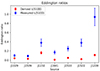 |
Fig. 6. Eddington ratios calculated using the measured continuum luminosity at 5100 Å (blue dots), and the derived continuum luminosity (red dots). The error bars that are not visible, due to their small values, are within the size of the dots. |
Two important conclusions can be drawn from such results. The first is that even without a strict host galaxy modeling, we can evaluate whether the host galaxy contaminates the continuum emission by analyzing the Eddington ratios calculated with the measured and derived continuum luminosity at 5100 Å. In the end, only J1522 showed a non-negligible host galaxy contamination. The second conclusion is the demonstration that the Eddington ratio obtained using the derived continuum luminosity is more reliable compared to the measured continuum luminosity approach, being less contaminated by relativistic jets and host galaxy emission. However, it is worth noting that the relations we used have a rather large standard deviation. This means that while they work for large samples, they may be misleading for a single source.
Even considering different sources of uncertainty in Eqs. (10) and (11), we have to keep in mind that we are estimating a bolometric luminosity only using a luminosity in a small range of wavelengths. This connection is based on the strong assumption that each value of Lλ(5100 Å) corresponds to a specific SED shape. To this end, Ferland et al. (2020) found that similar spectral features are not always related to the same SED shape. Some authors also found a positive correlation between the bolometric correction in Eq. (11) and the Eddington ratio (Vasudevan & Fabian 2007; Jin et al. 2012), a correlation disproved by Cheng et al. (2019), who also showed that the bolometric correction factor changes greatly according to the disk model assumed. The different Eddington ratios that can be obtained depending on the assumption made for the bolometric luminosity derivation (i.e., the scaling laws used) is clearly demonstrated for instance by comparing Berton et al. (2015) and Tortosa et al. (2023). The former derived the Eddington ratio from optical spectra, using scaling laws similar to those used in this work, while the latter derived the Eddington ratio from X-ray data. Looking at sources analyzed in both papers, the ϵ found in Tortosa et al. (2023) are three to four orders of magnitude larger than those found in Berton et al. (2015). Such huge difference cannot be entirely due to a variation in the accretion of the sources, especially on a timescale of a few years, but more likely on the approach used by the two papers. It is clear how the bolometric correction, and then the Eddington ratio, are just an estimation without precise knowledge of the SED shape. Therefore, our results should be taken with a grain of salt, and likely as a lower limit.
6.3. R4570-Eddington ratio discrepancy
An interesting parameter we can focus on is the R4570. The sources we analyzed turned out to belong to the populations A3 and A4 of the quasar main sequence, and therefore with a strong Fe II emission. Gaskell et al. (2007) with the Gaskell, Klimek & Nazarova BLR model showed that the Fe II emission comes from the outer part of the BLR, predominantly emitted at a radius twice that of Hβ. Moreover, Gaskell et al. (2022) stated that the Fe II emission is produced by photoionization, ruling out other possible hypotheses. They also found a positive correlation between the Fe II strength and the Eddington ratio (see also Boroson & Green 1992; Wandel & Boller 1998; Sulentic et al. 2000; Marziani et al. 2001). However, our sources seem to disagree with such a relation, except for J1228. As we describe, although they all belong to the A3 and A4 populations, the resulting Eddington ratios are close to the lower boundary for the NLS1s class. Also considering the discussed biases that could affect the Eddington ratio calculation, we can think that the high R4570 parameters might indicate higher Eddington ratios than we estimated. A higher Eddington ratio means a soft X-ray excess, which is not present in low Eddington ratio sources. Soft X-ray radiation breaks down the dust grains in the outer BLR, thus releasing the iron that then becomes photoionized by the photons coming from the accretion disk (Gaskell et al. 2022). Abramowicz & Fragile (2013) described that for a typical Shakura–Sunyaev disk, the viscous heating is balanced by radiative cooling. In high-Eddington ratio sources instead, the accretion disk does not have enough time to cool down only by the radiation losses; therefore, advective cooling is established. This forms the slim disk, in which the efficiency of transforming gravitational energy into radiative flux decreases with increasing accretion rate. A slim disk shows a moderate luminosity despite super-Eddington accretion. If this is the case, our sources could have higher Eddington ratios than we measured. This shows that the Eddington ratio estimate obtained via optical spectroscopy may be misleading, at least in some cases. The R4570 parameter may thus be a very important, and more reliable, indicator of the real Eddington ratios of some AGN.
6.4. SDSS-GTC spectral continuum comparison
Looking at the available SDSS spectra of the sample, we measured and compared the continuum flux densities only, and not the emission line properties, due to the much lower S/N compared to the GTC spectra. Computing the ratio of the flux densities at 5100 Å in Table 2, we found values between 0.90 for J1232 and 2.03 for J1641, the lowest and the highest, respectively. For J1232 the SDSS continuum is lower than the GTC continuum. In the remaining cases, however, the SDSS flux density is higher. In Seyfert galaxies, a variability of the flux density at 5100 Å, sometimes even much larger than 2, has been found in several studies (Zastrocky et al. 2024; Shapovalova et al. 2012; Grier et al. 2012). With a difference in the acquisition time of more than ten years between the SDSS and GTC spectra, these values are in agreement with the well-known long-term stochastic variability that characterizes all the AGN.
6.5. Comparison of the NLS1s properties
In Table 4 are reported the Pearson correlation coefficients we computed for several pairs of parameters, setting 0.05 as the threshold for the significance of the correlation analysis. We compared our results with the statistical analyses on large NLS1s samples available in the literature (Zhang et al. 2011; Rakshit et al. 2017; Paliya et al. 2024). The most significant correlations are those between Hα, Hβ, and [O III]λ5007 luminosity and the continuum luminosity at 5100 Å, with Pearson coefficients of around 0.8–0.9. This is in agreement to what was found by Rakshit et al. (2017) and Paliya et al. (2024). The same authors found, even though with a quite large scatter, a weak anti-correlation in the pairs of parameters of FWHM(Hβb)-R4570, FWHM(Hα)-R4570, and R5007-R4570, and a moderately strong anti-correlation between R5007 and L(Hβ). We found instead three strong correlations and one strong anti-correlation for the same couples of parameters. Nevertheless, the FWHM(Hβb)-R4570 and R5007-L(Hβ) correlation coefficients are not statistically significant, due to the p-values of 0.15 and 0.12, respectively. It is important to note that we did not consider the source J1641 in the FWHM(Hβb)-R4570 correlation test since the FWHM(Hβb) is much broader for intermediate Seyfert galaxies compared to NLS1s. Finally, we investigated the correlation between the Eddington ratios and the velocity shifts, with respect to the rest-frame wavelength, of the core and the strongest wing components in the [O III]λ5007, as found by Zhang et al. (2011). Nothing can be said in this case, due to the large p-values. Even though all the correlation coefficients are on average in agreement with the most recent literature, the extremely small number of sources we analyzed cannot represent a statistically valid sample. Nevertheless, the lack of noticeable peculiarities in the correlation analysis prove, once again, that these sources do not show deviations from the NLS1s class properties.
Pearson correlation coefficients.
7. Conclusions
In this study we derived the physical parameters of seven NLS1s, performing an analysis of the main emission lines in optical spectra observed with the GTC. The goal was to identify any common optical property of the sources in the sample that could explain why they show similar extreme features in the radio band. Investigating the most significant parameters, we did not find strong similarities between the sources. All but one showed classical behavior for the NLS1s class. Only J1641 turned out to be an intermediate Seyfert, but with physical properties that are common for this population. There are instead some shared traits. On average the black holes are more massive than the median value for the class (MBH = 1 × 10⁷, Cracco et al. 2016), with Eddington ratios much closer to the lower boundary for NLS1s. On the other hand, according to the R4570 parameter, the A3 and A4 nature of the sources (Sulentic & Marziani 2015) suggest an underestimation of the actual Eddington ratio, which could be much higher than we measured. High Eddington ratios for NLS1s could mean sources in an early stage of evolution, with an ongoing intense accretion activity. Though only the early evolutionary stage is not enough to explain why these sources show extreme flares in radio, it is an environment where the phenomena described by the hypotheses in Järvelä et al. (2024) can take place.
In particular AGN with a recently started activity, as NLS1s, can have regions with large amounts of gas, which is necessary to sustain a high Eddington ratio accretion (Mathur 2000). A gas-rich nuclear environment, coupled with the relatively massive black holes which might suggest the possible presence of relativistic jets, is in agreement with scenarios such as jet-cloud–star interaction, relativistic jet and free-free absorption with moving clouds, and magnetic reconnection in the jet (Järvelä et al. 2024). Nevertheless, with the results we obtained nothing more can be said to support or rule out some of the cited hypotheses.
To better strengthen the results we obtained in this study, optical spectra with wider wavelength ranges and higher S/N would be necessary. However, we would not expect much different results from those we obtained here since almost all the main emission lines were visible and we did not find substantial changes from the SDSS spectra. The only significant improvement we could make are spectra in which a host galaxy estimation can be made. In that case we could better constrain the Eddington ratio calculations. The similarities between the sources can be investigated more deeply with an analysis of the light curves, both in optical (Crepaldi et al., in prep.) and in radio frequencies. From the radio point of view, more observations at frequencies above 37 GHz would help us to better understand all the ongoing physical processes on these sources. Moreover, trigger observations, for example at high radio frequencies with the upgraded detectors of the Sardinia Radio Telescope or with other facilities such as the Square Kilometer Array, could add more constraints to the viable hypotheses we already mentioned.
Radio-quiet sources have a radio-loudness parameter, defined as the flux ratio F5 GHz/FB-band (Kellermann et al. 1989), lower than 10. On the other hand radio-loud sources have a radio-loudness parameter bigger than 10. The use of radio-loudness to identify jets should be, however, avoided, in favor of the more physical classification into jetted and non-jetted sources (Padovani 2017; Järvelä et al. 2017; Berton & Järvelä 2021).
Acknowledgments
The authors are grateful to the anonymous referee for the constructive comments. Based on observations made with the Gran Telescopio Canarias (GTC), installed at the Spanish Observatorio del Roque de los Muchachos of the Instituto de Astrofísica de Canarias, on the island of La Palma. L.C. and M.B. acknowledge the ESO Science Support Discretionary Fund. G.L.M. is supported by the Italian Research Center on High Performance Computing Big Data and Quantum Computing (ICSC), a project funded by the European Union – NextGenerationEU – and National Recovery and Resilience Plan (NRRP) – Mission 4 Component 2 within the activities of Spoke 3 (Astrophysics and Cosmos Observations). The authors are grateful to Dr. L. Foschini for the helpful discussion on the topic of bolometric luminosity derivation.
References
- Abdo, A. A., Ackermann, M., Ajello, M., et al. 2009a, ApJ, 699, 976 [CrossRef] [Google Scholar]
- Abdo, A. A., Ackermann, M., Ajello, M., et al. 2009b, ApJ, 707, L142 [NASA ADS] [CrossRef] [Google Scholar]
- Abramowicz, M. A., & Fragile, P. C. 2013, Liv. Rev. Rel., 16, 1 [Google Scholar]
- Ahn, S., & Fessler, J. A. 2003, Standard errors of mean, variance, and standard deviation estimators, Tech. Rep. 413, Comm. and Sign. Proc. Lab., Dept. of EECS, Univ. of Michigan, Ann Arbor, MI, 48109-2122 [Google Scholar]
- Antonucci, R., & Barvainis, R. 1988, ApJ, 332, L13 [Google Scholar]
- Barquín-González, L., Mateos, S., Carrera, F. J., et al. 2024, A&A, 687, A159 [NASA ADS] [CrossRef] [EDP Sciences] [Google Scholar]
- Becker, R. H., White, R. L., & Helfand, D. J. 1995, ApJ, 450, 559 [Google Scholar]
- Bentz, M. C., Peterson, B. M., Netzer, H., Pogge, R. W., & Vestergaard, M. 2009, ApJ, 697, 160 [Google Scholar]
- Bentz, M. C., Denney, K. D., Grier, C. J., et al. 2013, ApJ, 767, 149 [Google Scholar]
- Berton, M., & Järvelä, E. 2021, Astron. Nachr., 342, 1066 [NASA ADS] [CrossRef] [Google Scholar]
- Berton, M., Foschini, L., Ciroi, S., et al. 2015, A&A, 578, A28 [NASA ADS] [CrossRef] [EDP Sciences] [Google Scholar]
- Berton, M., Caccianiga, A., Foschini, L., et al. 2016a, A&A, 591, A98 [NASA ADS] [CrossRef] [EDP Sciences] [Google Scholar]
- Berton, M., Foschini, L., Ciroi, S., et al. 2016b, A&A, 591, A88 [NASA ADS] [CrossRef] [EDP Sciences] [Google Scholar]
- Berton, M., Congiu, E., Järvelä, E., et al. 2018, A&A, 614, A87 [NASA ADS] [CrossRef] [EDP Sciences] [Google Scholar]
- Berton, M., Björklund, I., Lähteenmäki, A., et al. 2020a, Contrib. Astron. Obs. Skalnate Pleso, 50, 270 [NASA ADS] [Google Scholar]
- Berton, M., Järvelä, E., Crepaldi, L., et al. 2020b, A&A, 636, A64 [NASA ADS] [CrossRef] [EDP Sciences] [Google Scholar]
- Berton, M., Peluso, G., Marziani, P., et al. 2021, A&A, 654, A125 [NASA ADS] [CrossRef] [EDP Sciences] [Google Scholar]
- Bicknell, G. V., Dopita, M. A., & O’Dea, C. P. O. 1997, ApJ, 485, 112 [NASA ADS] [CrossRef] [Google Scholar]
- Boroson, T. A., & Green, R. F. 1992, ApJS, 80, 109 [Google Scholar]
- Cardelli, J. A., Clayton, G. C., & Mathis, J. S. 1989, ApJ, 345, 245 [Google Scholar]
- Chamani, W., Savolainen, T., Hada, K., & Xu, M. H. 2021, A&A, 652, A14 [NASA ADS] [CrossRef] [EDP Sciences] [Google Scholar]
- Chen, S., Berton, M., La Mura, G., et al. 2018, A&A, 615, A167 [NASA ADS] [CrossRef] [EDP Sciences] [Google Scholar]
- Chen, S., Järvelä, E., Crepaldi, L., et al. 2020, MNRAS, 498, 1278 [NASA ADS] [CrossRef] [Google Scholar]
- Chen, S., Stevens, J. B., Edwards, P. G., et al. 2022, MNRAS, 512, 471 [Google Scholar]
- Cheng, H., Yuan, W., Liu, H.-Y., et al. 2019, MNRAS, 487, 3884 [NASA ADS] [CrossRef] [Google Scholar]
- Collin, S., Kawaguchi, T., Peterson, B. M., & Vestergaard, M. 2006, A&A, 456, 75 [NASA ADS] [CrossRef] [EDP Sciences] [Google Scholar]
- Condon, J. J., Cotton, W. D., Greisen, E. W., et al. 1998, AJ, 115, 1693 [Google Scholar]
- Cracco, V., Ciroi, S., Berton, M., et al. 2016, MNRAS, 462, 1256 [NASA ADS] [CrossRef] [Google Scholar]
- Dalla Barba, B., Berton, M., Foschini, L., et al. 2023, Physics, 5, 1061 [Google Scholar]
- Dalla Bontà, E., Peterson, B. M., Bentz, M. C., et al. 2020, ApJ, 903, 112 [CrossRef] [Google Scholar]
- Decarli, R., Dotti, M., Fontana, M., & Haardt, F. 2008, MNRAS, 386, L15 [NASA ADS] [Google Scholar]
- Dimitrijević, M. S., Popović, L. Č., Kovačević, J., Dačić, M., & Ilić, D. 2007, MNRAS, 374, 1181 [CrossRef] [Google Scholar]
- Dojčinović, I., Kovačević-Dojčinović, J., & Popović, L. Č. 2023, Adv. Space Res., 71, 1219 [CrossRef] [Google Scholar]
- Du, P., & Wang, J.-M. 2019, ApJ, 886, 42 [NASA ADS] [CrossRef] [Google Scholar]
- Ferland, G. J., Done, C., Jin, C., Landt, H., & Ward, M. J. 2020, MNRAS, 494, 5917 [Google Scholar]
- Foschini, L. 2011, in Narrow-Line Seyfert 1 Galaxies and their Place in the Universe, Proc. of Science, NLS1, 24 [Google Scholar]
- Foschini, L. 2014, Int. J. Mod. Phys. Conf. Ser., 28, 1460188 [NASA ADS] [CrossRef] [Google Scholar]
- Foschini, L. 2017, Front. Astron. Space Sci., 4, 6 [NASA ADS] [CrossRef] [Google Scholar]
- Foschini, L., Berton, M., Caccianiga, A., et al. 2015, A&A, 575, A13 [NASA ADS] [CrossRef] [EDP Sciences] [Google Scholar]
- Foschini, L., Ciroi, S., Berton, M., et al. 2019, Universe, 5, 199 [NASA ADS] [CrossRef] [Google Scholar]
- Foschini, L., Lister, M. L., Antón, S., et al. 2021, Universe, 7, 372 [NASA ADS] [CrossRef] [Google Scholar]
- Foschini, L., Lister, M. L., Andernach, H., et al. 2022, Universe, 8, 587 [NASA ADS] [CrossRef] [Google Scholar]
- Gaskell, C. M. 2009, NewAR, 53, 140 [NASA ADS] [CrossRef] [Google Scholar]
- Gaskell, C. M., Klimek, E. S., & Nazarova, L. S. 2007, in American Astronomical Society Meeting Abstracts, BAAS, 39, 947 [Google Scholar]
- Gaskell, M., Thakur, N., Tian, B., & Saravanan, A. 2022, Astron. Nachr., 343, e210112 [NASA ADS] [CrossRef] [Google Scholar]
- GRAVITY Collaboration (Sturm, E., et al.) 2018, Nature, 563, 657 [Google Scholar]
- Greene, J. E., & Ho, L. C. 2005, ApJ, 627, 721 [NASA ADS] [CrossRef] [Google Scholar]
- Greene, J. E., Hood, C. E., Barth, A. J., et al. 2010, ApJ, 723, 409 [NASA ADS] [CrossRef] [Google Scholar]
- Grier, C. J., Peterson, B. M., Pogge, R. W., et al. 2012, ApJ, 755, 60 [NASA ADS] [CrossRef] [Google Scholar]
- Grupe, D., Komossa, S., Leighly, K. M., & Page, K. L. 2010, ApJS, 187, 64 [NASA ADS] [CrossRef] [Google Scholar]
- Guainazzi, M., Matt, G., & Perola, G. C. 2005, A&A, 444, 119 [NASA ADS] [CrossRef] [EDP Sciences] [Google Scholar]
- Heinz, S., & Sunyaev, R. A. 2003, MNRAS, 343, L59 [Google Scholar]
- Helfand, D. J., White, R. L., & Becker, R. H. 2015, ApJ, 801, 26 [NASA ADS] [CrossRef] [Google Scholar]
- Ilić, D., Shapovalova, A. I., Popović, L. Č., et al. 2017, Front. Astron. Space Sci., 4, 12 [CrossRef] [Google Scholar]
- Järvelä, E., Lähteenmäki, A., & León-Tavares, J. 2015, A&A, 573, A76 [NASA ADS] [CrossRef] [EDP Sciences] [Google Scholar]
- Järvelä, E., Lähteenmäki, A., Lietzen, H., et al. 2017, A&A, 606, A9 [NASA ADS] [CrossRef] [EDP Sciences] [Google Scholar]
- Järvelä, E., Lähteenmäki, A., & Berton, M. 2018, A&A, 619, A69 [NASA ADS] [CrossRef] [EDP Sciences] [Google Scholar]
- Järvelä, E., Berton, M., & Crepaldi, L. 2021, Front. Astron. Space Sci., 8, 147 [CrossRef] [Google Scholar]
- Järvelä, E., Savolainen, T., Berton, M., et al. 2024, MNRAS, 532, 3069 [CrossRef] [Google Scholar]
- Jin, C., Ward, M., & Done, C. 2012, MNRAS, 425, 907 [NASA ADS] [CrossRef] [Google Scholar]
- Kalberla, P. M. W., Burton, W. B., Hartmann, D., et al. 2005, A&A, 440, 775 [NASA ADS] [CrossRef] [EDP Sciences] [Google Scholar]
- Kaspi, S., Smith, P. S., Netzer, H., et al. 2000, ApJ, 533, 631 [Google Scholar]
- Kellermann, K. I., Sramek, R., Schmidt, M., Shaffer, D. B., & Green, R. 1989, AJ, 98, 1195 [Google Scholar]
- Kollatschny, W., & Zetzl, M. 2011, Nature, 470, 366 [NASA ADS] [CrossRef] [Google Scholar]
- Kollatschny, W., & Zetzl, M. 2013, A&A, 558, A26 [NASA ADS] [CrossRef] [EDP Sciences] [Google Scholar]
- Komatsu, E., Smith, K. M., Dunkley, J., et al. 2011, ApJS, 192, 18 [Google Scholar]
- Komossa, S., Xu, D., Zhou, H., Storchi-Bergmann, T., & Binette, L. 2008, ApJ, 680, 926 [NASA ADS] [CrossRef] [Google Scholar]
- Kovačević, J., Popović, L. Č., & Dimitrijević, M. S. 2010, ApJS, 189, 15 [Google Scholar]
- Lähteenmäki, A., Järvelä, E., Hovatta, T., et al. 2017, A&A, 603, A100 [NASA ADS] [CrossRef] [EDP Sciences] [Google Scholar]
- Lähteenmäki, A., Järvelä, E., Ramakrishnan, V., et al. 2018, A&A, 614, L1 [NASA ADS] [CrossRef] [EDP Sciences] [Google Scholar]
- La Mura, G., Popović, L. Č., Ciroi, S., Rafanelli, P., & Ilić, D. 2007, ApJ, 671, 104 [NASA ADS] [CrossRef] [Google Scholar]
- Laor, A. 2000, ApJ, 543, L111 [NASA ADS] [CrossRef] [Google Scholar]
- Letawe, G., Magain, P., Courbin, F., et al. 2007, MNRAS, 378, 83 [NASA ADS] [CrossRef] [Google Scholar]
- Lister, M. L., Aller, M. F., Aller, H. D., et al. 2016, AJ, 152, 12 [NASA ADS] [CrossRef] [Google Scholar]
- Malkan, M. A., Gorjian, V., & Tam, R. 1998, ApJS, 117, 25 [Google Scholar]
- Mandal, A. K., Rakshit, S., Stalin, C. S., et al. 2021, MNRAS, 502, 2140 [NASA ADS] [CrossRef] [Google Scholar]
- Marziani, P., Sulentic, J. W., Zwitter, T., Dultzin-Hacyan, D., & Calvani, M. 2001, ApJ, 558, 553 [NASA ADS] [CrossRef] [Google Scholar]
- Marziani, P., Zamanov, R. K., Sulentic, J. W., & Calvani, M. 2003, MNRAS, 345, 1133 [NASA ADS] [CrossRef] [Google Scholar]
- Marziani, P., Martínez Carballo, M. A., Sulentic, J. W., et al. 2016, Ap&SS, 361, 29 [NASA ADS] [CrossRef] [Google Scholar]
- Marziani, P., del Olmo, A., D’Onofrio, M., et al. 2018a, in Proceedings of Science, vol. Revisiting narrow-line Seyfert 1 galaxies and their place in the Universe, 2 [Google Scholar]
- Marziani, P., Dultzin, D., Sulentic, J. W., et al. 2018b, Front. Astron. Space Sci., 5, 6 [CrossRef] [Google Scholar]
- Marziani, P., Berton, M., Panda, S., & Bon, E. 2021, Universe, 7, 484 [NASA ADS] [CrossRef] [Google Scholar]
- Mathur, S. 2000, MNRAS, 314, L17 [NASA ADS] [CrossRef] [Google Scholar]
- Netzer, H. 2019, MNRAS, 488, 5185 [NASA ADS] [CrossRef] [Google Scholar]
- Olguín-Iglesias, A., Kotilainen, J., & Chavushyan, V. 2020, MNRAS, 492, 1450 [Google Scholar]
- Osterbrock, D. E. 1977, ApJ, 215, 733 [Google Scholar]
- Osterbrock, D. E. 1991, Rep. Prog. Phys., 54, 579 [Google Scholar]
- Osterbrock, D. E., & Koski, A. T. 1976, MNRAS, 176, 61P [NASA ADS] [CrossRef] [Google Scholar]
- Osterbrock, D. E., & Pogge, R. W. 1985, ApJ, 297, 166 [Google Scholar]
- Padovani, P. 2017, Nat. Astron., 1, 0194 [Google Scholar]
- Paliya, V. S., Parker, M. L., Jiang, J., et al. 2019, ApJ, 872, 169 [NASA ADS] [CrossRef] [Google Scholar]
- Paliya, V. S., Stalin, C. S., Domínguez, A., & Saikia, D. J. 2024, MNRAS, 527, 7055 [Google Scholar]
- Peterson, B. M. 2011, in Narrow-Line Seyfert 1 Galaxies and their Place in the Universe, 32 [Google Scholar]
- Peterson, B., & Dalla Bontà, E. 2018, in Proceedings of Science, vol. Revisiting narrow-line Seyfert 1 galaxies and their place in the Universe, 8 [Google Scholar]
- Peterson, B. M., & Wandel, A. 1999, ApJ, 521, L95 [NASA ADS] [CrossRef] [Google Scholar]
- Peterson, B. M., Ferrarese, L., Gilbert, K. M., et al. 2004, ApJ, 613, 682 [Google Scholar]
- Proga, D., Stone, J. M., & Kallman, T. R. 2000, ApJ, 543, 686 [Google Scholar]
- Rakshit, S., Stalin, C. S., Chand, H., & Zhang, X.-G. 2017, ApJS, 229, 39 [Google Scholar]
- Richards, J. L., & Lister, M. L. 2015, ApJ, 800, L8 [NASA ADS] [CrossRef] [Google Scholar]
- Romano, P., Vercellone, S., Foschini, L., et al. 2018, MNRAS, 481, 5046 [NASA ADS] [CrossRef] [Google Scholar]
- Romano, P., Lähteenmäki, A., Vercellone, S., et al. 2023, A&A, 673, A85 [NASA ADS] [CrossRef] [EDP Sciences] [Google Scholar]
- Sani, E., Lutz, D., Risaliti, G., et al. 2010, MNRAS, 403, 1246 [Google Scholar]
- Schmidt, E. O., Oio, G. A., Ferreiro, D., Vega, L., & Weidmann, W. 2018, A&A, 615, A13 [NASA ADS] [CrossRef] [EDP Sciences] [Google Scholar]
- Shapovalova, A. I., Popović, L. Č., Burenkov, A. N., et al. 2012, ApJS, 202, 10 [NASA ADS] [CrossRef] [Google Scholar]
- Shen, Y., & Ho, L. C. 2014, Nature, 513, 210 [NASA ADS] [CrossRef] [Google Scholar]
- Shen, Y., Grier, C. J., Horne, K., et al. 2024, ApJS, 272, 26 [NASA ADS] [CrossRef] [Google Scholar]
- Sulentic, J., & Marziani, P. 2015, Front. Astron. Space Sci., 2, 6 [NASA ADS] [CrossRef] [Google Scholar]
- Sulentic, J. W., Zwitter, T., Marziani, P., & Dultzin-Hacyan, D. 2000, ApJ, 536, L5 [Google Scholar]
- Tortosa, A., Ricci, C., Tombesi, F., et al. 2022, MNRAS, 509, 3599 [Google Scholar]
- Tortosa, A., Ricci, C., Ho, L. C., et al. 2023, MNRAS, 519, 6267 [NASA ADS] [CrossRef] [Google Scholar]
- Varglund, I., Järvelä, E., Lähteenmäki, A., et al. 2022, A&A, 668, A91 [NASA ADS] [CrossRef] [EDP Sciences] [Google Scholar]
- Vasudevan, R. V., & Fabian, A. C. 2007, MNRAS, 381, 1235 [NASA ADS] [CrossRef] [Google Scholar]
- Vietri, A., Berton, M., Ciroi, S., et al. 2018, in Proceedings of Science, vol., 47 [Google Scholar]
- Vietri, A., Berton, M., Järvelä, E., et al. 2024, A&A, 689, A123 [NASA ADS] [CrossRef] [EDP Sciences] [Google Scholar]
- Wandel, A., & Boller, T. 1998, A&A, 331, 884 [NASA ADS] [Google Scholar]
- Williams, R. J., Pogge, R. W., & Mathur, S. 2002, AJ, 124, 3042 [CrossRef] [Google Scholar]
- Williams, R. J., Mathur, S., & Pogge, R. W. 2004, ApJ, 610, 737 [NASA ADS] [CrossRef] [Google Scholar]
- Xu, D., Komossa, S., Zhou, H., et al. 2012, AJ, 143, 83 [NASA ADS] [CrossRef] [Google Scholar]
- Zamanov, R., Marziani, P., Sulentic, J. W., et al. 2002, ApJ, 576, L9 [NASA ADS] [CrossRef] [Google Scholar]
- Zastrocky, T. E., Brotherton, M. S., Du, P., et al. 2024, ApJS, 272, 29 [NASA ADS] [CrossRef] [Google Scholar]
- Zhang, K., Dong, X.-B., Wang, T.-G., & Gaskell, C. M. 2011, ApJ, 737, 71 [NASA ADS] [CrossRef] [Google Scholar]
- Zhou, H., Wang, T., Yuan, W., et al. 2006, ApJS, 166, 128 [NASA ADS] [CrossRef] [Google Scholar]
Appendix A: Tables, spectra and line profiles
Observational and physical parameters derived from the optical spectra.
[O III]λλ4959,5007 model parameters.
Hβ model parameters.
Hα+[N II]λλ6548,6583 and [S II]λλ6716,6731 model parameters.
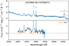 |
Fig. A.1. Spectrum of J1029. |
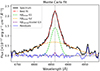 |
Fig. A.2. Hβ line profile of J1029. |
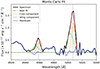 |
Fig. A.3. [O III]λλ4959,5007 line profile of J1029. |
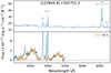 |
Fig. A.4. Spectrum of J1228. |
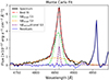 |
Fig. A.5. β line profile of J1228. |
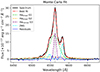 |
Fig. A.6. Hα+[N II]λλ6548,6583 line profiles of J1228. |
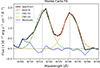 |
Fig. A.7. [S II]λλ6716,6731 line profiles of J1228. |
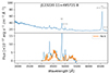 |
Fig. A.8. Spectrum of J1232. |
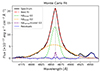 |
Fig. A.9. Hβ line profile of J1232. |
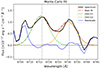 |
Fig. A.10. [S II]λλ6716,6731 line profiles of J1232. |
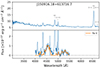 |
Fig. A.11. Spectrum of J1509. |
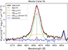 |
Fig. A.12. Hβ line profile of J1509. |
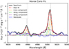 |
Fig. A.13. [O III]λλ4959,5007 line profiles of J1509. |
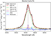 |
Fig. A.14. Hα+[N II]λλ6548,6583 line profiles of J1509. |
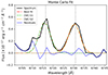 |
Fig. A.15. [S II]λλ6716,6731 line profiles of J1509. |
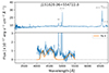 |
Fig. A.16. Spectrum of J1510. |
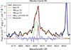 |
Fig. A.17. Hβ line profile of J1510. |
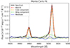 |
Fig. A.18. [O III]λλ4959,5007 line profiles of J1510. |
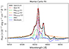 |
Fig. A.19. Hα+[N II]λλ6548,6583 line profiles of J1510. |
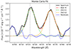 |
Fig. A.20. [S II]λλ6716,6731 line profiles of J1510. |
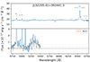 |
Fig. A.21. Spectrum of J1522. |
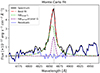 |
Fig. A.22. Hβ line profile of J1522. |
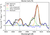 |
Fig. A.23. [O III]λλ4959,5007 line profiles of J1522. |
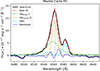 |
Fig. A.24. Hα+[N II]λλ6548,6583 line profiles of J1522. |
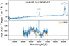 |
Fig. A.25. Spectrum of J1641. |
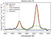 |
Fig. A.26. [O III]λλ4959,5007 line profiles of J1641. |
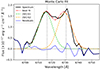 |
Fig. A.27. [S II]λλ6716,6731 line profiles of J1641. |
All Tables
All Figures
|
Fig. 1. [O III]λλ4959,5007 emission lines of J1641. The light gray shaded regions represent the ranges where the χ2 is assessed. |
| In the text | |
|
Fig. 2. [O III]λλ4959,5007 line profiles of J1228. |
| In the text | |
|
Fig. 3. Hα+[N II]λλ6548,6583 line profiles of J1232. The cyan dashed line represents the [N II] line profiles, which are much fainter than the Hα emission. |
| In the text | |
|
Fig. 4. [O III]λλ4959,5007 line profiles of J1232, which show wing components stronger than the core components. |
| In the text | |
|
Fig. 5. Hβ line profile of J1641. The broad and narrow components have a FWHM of 4050 km s−1 and 493 km s−1, respectively. |
| In the text | |
|
Fig. 6. Eddington ratios calculated using the measured continuum luminosity at 5100 Å (blue dots), and the derived continuum luminosity (red dots). The error bars that are not visible, due to their small values, are within the size of the dots. |
| In the text | |
|
Fig. A.1. Spectrum of J1029. |
| In the text | |
|
Fig. A.2. Hβ line profile of J1029. |
| In the text | |
|
Fig. A.3. [O III]λλ4959,5007 line profile of J1029. |
| In the text | |
|
Fig. A.4. Spectrum of J1228. |
| In the text | |
|
Fig. A.5. β line profile of J1228. |
| In the text | |
|
Fig. A.6. Hα+[N II]λλ6548,6583 line profiles of J1228. |
| In the text | |
|
Fig. A.7. [S II]λλ6716,6731 line profiles of J1228. |
| In the text | |
|
Fig. A.8. Spectrum of J1232. |
| In the text | |
|
Fig. A.9. Hβ line profile of J1232. |
| In the text | |
|
Fig. A.10. [S II]λλ6716,6731 line profiles of J1232. |
| In the text | |
|
Fig. A.11. Spectrum of J1509. |
| In the text | |
|
Fig. A.12. Hβ line profile of J1509. |
| In the text | |
|
Fig. A.13. [O III]λλ4959,5007 line profiles of J1509. |
| In the text | |
|
Fig. A.14. Hα+[N II]λλ6548,6583 line profiles of J1509. |
| In the text | |
|
Fig. A.15. [S II]λλ6716,6731 line profiles of J1509. |
| In the text | |
|
Fig. A.16. Spectrum of J1510. |
| In the text | |
|
Fig. A.17. Hβ line profile of J1510. |
| In the text | |
|
Fig. A.18. [O III]λλ4959,5007 line profiles of J1510. |
| In the text | |
|
Fig. A.19. Hα+[N II]λλ6548,6583 line profiles of J1510. |
| In the text | |
|
Fig. A.20. [S II]λλ6716,6731 line profiles of J1510. |
| In the text | |
|
Fig. A.21. Spectrum of J1522. |
| In the text | |
|
Fig. A.22. Hβ line profile of J1522. |
| In the text | |
|
Fig. A.23. [O III]λλ4959,5007 line profiles of J1522. |
| In the text | |
|
Fig. A.24. Hα+[N II]λλ6548,6583 line profiles of J1522. |
| In the text | |
|
Fig. A.25. Spectrum of J1641. |
| In the text | |
|
Fig. A.26. [O III]λλ4959,5007 line profiles of J1641. |
| In the text | |
|
Fig. A.27. [S II]λλ6716,6731 line profiles of J1641. |
| In the text | |
Current usage metrics show cumulative count of Article Views (full-text article views including HTML views, PDF and ePub downloads, according to the available data) and Abstracts Views on Vision4Press platform.
Data correspond to usage on the plateform after 2015. The current usage metrics is available 48-96 hours after online publication and is updated daily on week days.
Initial download of the metrics may take a while.