| Issue |
A&A
Volume 698, June 2025
|
|
|---|---|---|
| Article Number | A320 | |
| Number of page(s) | 14 | |
| Section | Extragalactic astronomy | |
| DOI | https://doi.org/10.1051/0004-6361/202452421 | |
| Published online | 24 June 2025 | |
Interaction of the relativistic jet and the narrow-line region of PMN J0948+0022
1
European Southern Observatory (ESO), Alonso de Córdova 3107, Vitacura Santiago, Chile
2
Università degli Studi dell’Insubria, Via Valleggio 11, Como 22100, Italy
3
Osservatorio Astronomico di Brera, Istituto Nazionale di Astrofisica (INAF), Via E. Bianchi 46, Merate (LC) 23807, Italy
4
Università degli Studi di Padova, Vicolo dell’Osservatorio 3, Padova 35122, Italy
5
Scuola Normale Superiore, Piazza dei Cavalieri 7, Pisa 56126, Italy
6
Osservatorio Astrofisico di Arcetri, Istituto Nazionale di Astrofisica (INAF), Largo E. Fermi 5, Firenze 50125, Italy
7
School of Physics, University of Melbourne, Parkville, Victoria 3010, Australia
8
Osservatorio Astronomico di Padova, Istituto Nazionale di Astrofisica (INAF), Vicolo dell’Osservatorio, 5 Padova (PD) 35122, Italy
⋆ Corresponding author.
Received:
30
September
2024
Accepted:
17
May
2025
Abstract
We analyzed publicly available optical spectra of PMN J0948+0022 obtained with the Sloan Digital Sky Survey, the X-shooter, and the Multi Unit Spectroscopic Explorer (MUSE). Initially, PMN J0948+0022 was classified as a jetted narrow-line Seyfert 1 galaxy, but X-shooter and MUSE observations, which have a better spectral resolution, revealed a different profile for the Hβ line: from a Lorentzian to a composite one (a combination of a broad and a narrow Gaussian), which is more typical of intermediate Seyfert galaxies. According to the unified model, intermediate Seyferts are viewed at larger angles. However, we show that, in this case, the composite line profile results from the interaction of the powerful relativistic jet with the narrow-line region. The jet transfers part of its kinetic energy to the narrow-line region, producing flux changes in the Hβ narrow component (a drop by a factor of 3.4 from SDSS to X-shooter), the [O III]λ5007 core component (which nearly doubled from X-shooter to MUSE), and its blue wing (Δv ∼ 200 km s−1), which we interpret as evidence of an outflow. We also recalculated the physical parameters of this AGN, obtaining a black hole mass of 107.8 M⊙ and an Eddington ratio of ∼0.21 (weighted mean).
Key words: galaxies: active / galaxies: jets / galaxies: nuclei / galaxies: Seyfert
© The Authors 2025
 Open Access article, published by EDP Sciences, under the terms of the Creative Commons Attribution License (https://creativecommons.org/licenses/by/4.0), which permits unrestricted use, distribution, and reproduction in any medium, provided the original work is properly cited.
This article is published in open access under the Subscribe to Open model. This email address is being protected from spambots. You need JavaScript enabled to view it. to support open access publication.
1. Introduction
Classically, jetted active galactic nuclei (AGN) are divided into two main categories: radio galaxies and blazars. Blazars are further subdivided into BL Lac objects (BL Lacs) and flat-spectrum radio quasars (FSRQs), depending on the properties of their optical lines (Blandford et al. 2019). Physically, FSRQs are characterized by efficient accretion and a high-density circumnuclear environment, while BL Lacs typically display inefficient accretion and a low-density circumnuclear environment. This scenario, known as the blazar sequence (Fossati et al. 1998; Ghisellini et al. 1998), was revised when, in 2008, another class of high-energy jetted AGN was discovered: jetted narrow-line Seyfert 1 galaxies (NLS1s). Before 2008, all known NLS1s had not been detected in γ-rays and, consequently, were not associated with a powerful jet emission. These objects are classified according to the following criteria: a broad Hβ line with full width at half maximum (FWHM) (Hβ) ≲ 2000 km s−1, weak oxygen lines with [O III]/Hβ ≲ 3, and a significant iron emission (Osterbrock & Pogge 1985; Goodrich 1989). Similar to FSRQs, jetted NLS1s are characterized by an efficient accretion process, but they exhibit relatively low black hole (BH) masses (∼107 M⊙). In contrast, both BL Lacs and FSRQs are characterized by more massive black holes (∼108 − 9 M⊙). There is still an ongoing debate about the actual black hole mass range for NLS1s (∼106 − 8 M⊙ versus ∼108 − 9 M⊙); see, for example, (Foschini 2020). In this context, γ-ray emitting NLS1s represent a new class of objects that challenge the well-established theories and classifications proposed in recent years.
The first object classified as a jetted NLS1 is PMN J0948+0022 (z = 0.585 ± 0.0011). Its first optical spectrum (Williams et al. 2002; Zhou et al. 2003) revealed typical NLS1 characteristics: FWHM(Hβ) = (1500 ± 55) km s−1, [O III]/Hβ < 3, and significant Fe II emission (Zhou et al. 2003). At the same time, PMN J0948+0022 exhibited remarkable radio activity for an NLS1 (Zhou et al. 2003). The inverted spectrum and high brightness temperature suggested a relativistic jet closely aligned with the observer’s line of sight, which was confirmed by detections from the Fermi Gamma-ray Space Telescope (Abdo et al. 2009a,b; Foschini et al. 2010), with a jet angle of θ ∼ 3 − 6° (Abdo et al. 2009b; Foschini et al. 2012). Additionally, the jets exhibit both parsec- and kiloparsec-scale structures (Doi et al. 2012; Lister et al. 2016), with superluminal speeds of 11.5c.
Between 2008 and 2016, PMN J0948+0022 was particularly active in the radio and γ-ray bands, experiencing two major outbursts. The first occurred in July 2010, reaching an isotropic luminosity of 1048 erg s−1 (Donato 2010; Foschini et al. 2011), and the second occurred in January 2013, with a luminosity of 1.5 × 1048 erg s−1 (D’Ammando et al. 2015). Extensive multiwavelength monitoring campaigns began shortly after the discovery and gained interest following the first flare, revealing significant variability across multiple bands (Abdo et al. 2009a; Foschini et al. 2011, 2012; D’Ammando et al. 2014; Angelakis et al. 2015; Lähteenmäki et al. 2017; Yao & Komossa 2023; Xin et al. 2022), a common feature of jetted AGNs. These studies documented intra-night optical variability (INOV) and mid-infrared variability (Liu et al. 2010; Mao 2021; Ojha et al. 2021, 2022), as well as quasiperiodic oscillations in the Fermi-Large Area Telescope energy band (Zhang et al. 2017). The INOV is thought to be related to relativistic beaming (Ojha et al. 2022), while the quasiperiodic oscillations of ∼490 days are likely linked to jet structures (Zhang et al. 2017).
The X-ray spectrum of PMN J0948+0022 is also variable, with a photon index Γ ranging from 1.3 to 1.8 (Foschini et al. 2015). The spectrum is characterized by a soft excess below 2.5 keV, possibly associated with thermal Comptonization (a typical Seyfert emission), and a potential power-law component at higher energies likely originating from the relativistic jet (Bhattacharyya et al. 2014; Berton et al. 2019).
The host galaxy of PMN J0948+0022 exhibits a brightness profile with a Sérsic index of n < 2 for the bulge component (Olguín-Iglesias et al. 2020), suggesting a disk-like morphology, which is typical of NLS1 galaxies (e.g., Varglund et al. 2023).
Since the discovery of PMN J0948+0022 as a γ-NLS1, about two dozen objects of this type have been identified (Foschini et al. 2022), suggesting that these are not rare but instead form a significant subclass of AGN. Jetted NLS1 galaxies share several properties with other jetted AGNs, including double-peaked spectral energy distributions (Abdo et al. 2009b), variable flat or inverted radio spectra (Angelakis et al. 2015; Lähteenmäki et al. 2017), core-jet morphology (Doi et al. 2006; Giroletti et al. 2011), and superluminal motion (Lister et al. 2016). The key connection between the different families of jetted AGNs likely lies in their evolutionary stage. The NLS1 galaxies are thought to be young or rejuvenated quasars (Mathur 2000), potentially representing the progenitors of more evolved quasars (Berton et al. 2016, 2017).
In this paper we analyze the optical spectral variations of the emission lines, particularly Hβ and [O III]λλ4959,5007, of PMN J0948+0022. We find a variation in the flux of the [O III]λ5007 core component and outflow, along with a variation in the outflow velocity. We also propose a reclassification of this AGN from an NLS1 to an intermediate Seyfert (IS), as the improved spectral resolution of X-shooter and Multi-Unit Spectroscopic Explorer (MUSE) allowed us to disentangle the narrow and the broad components of Hβ. The reclassification, combined with the small jet viewing angles reported by Abdo et al. (2009b), Foschini et al. (2012), Doi et al. (2019), makes PMN J0948+0022 a peculiar case in which the geometric interpretation of the AGN provided by the unified model (UM) (Keel 1980; Antonucci 1993; Urry & Padovani 1995) raises intriguing doubts.
This paper is divided as follows. In Sect. 2 we present the optical spectral observations of PMN J0948+0022 from the Sloan Digital Sky Survey (SDSS) in 2000, the X-shooter (European Southern Observatory-Very Large Telescope-Unit Telescope 3, ESO-VLT-UT3) in 2017, and the MUSE (ESO-VLT-UT4) in 2022−2023. In Sect. 3 we present the data analysis of the mentioned spectra with a description of the fitting procedure. In Sect. 4 we present the results of the analysis: the reclassification of PMN J0948+0022, the variations in the Hβ profile, the variations in the [O III]λ5007 core and wing fluxes, the estimation of the physical parameters (black hole mass, MBH, and Eddington ratio, REdd), and the calculation of the geometrical parameters (sublimation, outer, and NLR radii). In Sect. 5 we discuss the physical explanation of the decrease in flux of the Hβ line and of the [O III]λ5007 line. Lastly, in Sect. 6 we summarize the main results and present the conclusions. Throughout this paper, we adopt a standard ΛCDM cosmology with: H0 = 73.3 km s−1 Mpc−1, Ωmatter = 0.3, and Ωvacuum = 0.7 (Riess et al. 2022).
2. Observations and data reduction
The optical spectroscopic observations of PMN J0948+0022 can be grouped into three periods: in 2000 from SDSS, in 2017 from X-shooter, and finally between November 24, 2022, and March 8, 2023, from MUSE. All of these data are publicly available. The analysis is presented in the following sections separately, for a summary see Table 1. The three redshift-corrected (z ∼ 0.5850) spectra are plotted in Fig. 1.
Analyzed observations of PMN J0948+0022.
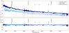 |
Fig. 1. Top: Three redshift-corrected spectra in the visible range. Bottom: Three redshift-corrected spectra, with the continuum and iron lines subtracted shown. The X-shooter spectrum is composed of three sections, but here we report only the one useful for the comparison with the SDSS and MUSE spectra. In both panels, we present the SDSS spectrum in light blue, the X-shooter spectrum in blue, and the MUSE spectrum in magenta. The vertical lines correspond to the identified optical lines with a significance > 5σ in all the spectra, except for [O III]λ5007, which was included even though it was not detected in the SDSS spectrum. |
2.1. SDSS (2000)
PMN J0948+0022 (SDSS J094857.32+002225.5) was observed twice in 2000, the first time on February 28, 2000 (MJD 51602), and the second on March 27, 2000 (MJD 51630). The observing time was 3600 s for both observations with a spectral coverage of 3800−9200 Å and coordinates (RA, Dec) = (147.2389, 0.3738) deg. The SDSS spectrograph is a multi-fiber instrument (640 fibers in total) covering a projected scale of 3 arcsec, the physical scale for this object is s = 6.31 kpc/arcsec2. According to Olguín-Iglesias et al. (2020) the effective radius for the bulge of the host galaxy of PMN J0948+0022 is ∼1.82−0.90 kpc (J − K band). This implies that the entire AGN is included within the SDSS aperture. The reduced spectra can be found in the SDSS SkyServer DR183. Here, we used the second observation (MJD 51630) due to the SDSS automatic classification of observations (see the “sciencePrimary” label in the archive).
2.2. X-shooter (2017)
The object was observed on December 22, 2017 (MJD 58109), with 42 exposures of 235 s each, for a total of approximately 2.7 hours. The spectral coverage of the instrument is divided into three arms, as the instrument itself: ultraviolet (3000–5600 Å), visible (5500–10 200 Å), and near-infrared arm (10 200–24 800 Å). This broad spectral coverage allowed us to obtain multiple lines in the X-shooter spectrum (see, for example, Table A.1). The pointing was centered at (RA, Dec) = (147.2389, 0.3731) deg, in a slightly different position with respect to the SDSS. However, due to the distance of the object and considering the slit width (1.2″), we can conclude that the AGN was completely included in the observation (effective radius for the bulge emission of ∼0.6 − 0.3″, see again Olguín-Iglesias et al. 2020).
The data are publicly available in the ESO archive4. To combine and reduce the spectra, we used the X-shooter ESO pipeline EsoReflex version 3.5.2 (for details, see the documentation of the latest version5). The data reduction was performed using standard procedures, except for the extraction radius of the 1D spectrum obtained from the 2D exposure. A smaller extraction region was selected to minimize potential contamination from the host galaxy. For this purpose, we defined the extraction region based on the observing seeing conditions on December 22, 2017, as the observations were seeing-limited. During that night, the seeing varied between 0.56″ and 0.36″ (see Table 1). To be conservative, we adopted 0.6″ (FWHM) as a reference and converted it into pixels using a scale of 0.158″/px (see the spectrograph characteristics6). The final extraction radius is 5 px (compared the default one of the pipeline, which is 15 px). The extraction procedure was conducted using IRAF version 2.18. Lastly, we obtained three FITS files, corresponding to the three arms of the spectrograph: NIR, visible, and UV.
2.3. MUSE (2022–2023)
MUSE is an integral field spectrograph covering the spectral range 4650−9300 Å, producing data cubes with a 1 × 1 arcmin2 field of view (FoV) in wide field mode (WFM). These data cubes have two spatial dimensions (x, y) and one spectrum per pixel (see Fig. C.1), where the spectral information is stored along the z-axis. MUSE observations of PMN J0948+0022 were carried in the WFM without adaptive optics (NOAO). The object was observed multiple times and under different conditions; for details, see Table 1. We rejected the observations from November 25 and February 9−10 from the analysis due to poor data quality mainly related to the atmospheric conditions (observations conducted with clouds, or aborted for the same reason). The reduction of the spectra, similarly to the X-shooter case, was carried out with the MUSE ESO pipeline (EsoReflex) version 2.8.5. The final products are single reduced exposures and the combined data cube. Before the spectra extraction, we applied CubePCA7, a package developed for cleaning astronomical IFU observations – particularly MUSE data cubes – from sky line residuals and systematic artifacts. The core concept of CubePCA is to select a reference region in the cube (top left in our case) to represent the sky, create a mask, and apply Principal Component Analysis (PCA) to subtract the sky contribution from the entire cube. After this cleaning step, we extracted the spectrum from a circular region with a radius ranging from 4 to 9 pixels, centered at (RA, Dec) = (147.2388, 0.3738) deg. This differential extraction allowed us to account for the different weather conditions, using larger extraction radii for the worst seeing conditions (such as those on January 28, 2023) and smaller radii for the best cases (such as those on March 8, 2023), see Table 1. Given the point-like nature of the source, we converted each seeing (interpreted as a FWHM) into pixels to ensure that only the AGN contribution was included in the extracted spectrum. The pixel scale of 0.2″/px confirms that, in all cases, the observations are seeing-limited. We then inspected the individual MUSE spectra and compared the Hβ–[O III]λ5007 profiles. From individual spectra, we confirmed that the line fluxes do not vary significantly (≲2σ) during the time spanned by the observations. Keeping in mind this, we combined the individual MUSE spectra using a weighted average, where the weights were determined by the continuum fluctuations in the 5050−5150 Å range. This procedure allowed us to reduce the uncertainties of the flux.
3. Data analysis
3.1. Methodology
We performed line identification in the PMN J0948+0022 spectra. We set the significance level at 5σ, only the lines that met this threshold were used to calculate the weighted mean for the redshift (see Table A.2). Here, σ is the standard deviation of the line-free continuum in the 5050−5150 Å range. For [O II]λ3727, Hβ, [O III]λ5007, Hα, and [N II]λ6583 (when present) we performed an accurate fitting, described in Sect. 3.2, the results of which are reported in Table A.1 where we listed: the identified lines with the observed wavelength (λobs), the flux, and the FWHM.
We corrected the wavelength by the redshift using the [O II]λ3727 line, which is the [O II]λ3726,3729 doublet in the X-shooter and MUSE cases, and a single line in the SDSS case. The difference is due to the limited spectral resolution of the instrument. We chose [O II]λ3727 because of its presence in all the spectra and its significance with respect to [O III]λ5007. From its displacement, we obtained: z = (0.5857 ± 0.0001) in SDSS, z = (0.5850 ± 0.0001) in X-shooter, and z = (0.5850 ± 0.0004) in MUSE. Each value is in agreement with the public value of z = 0.585.
For the modeling of the continuum, host galaxy, and iron components, we used AGN FANTASY (Fully Automated pythoN tool for AGN Spectra analYsis)8 (Ilić et al. 2020, 2023; Rakić 2022). This tool is based on the Levenberg-Marquardt algorithm, implemented through the sherpa Python package, and optimized for simultaneous multicomponent fitting of the AGN spectra. The continuum was found to be AGN-dominated and was fit with a power law with a spectral index of ∼3. The host-galaxy contribution was negligible. For the modeling of the iron lines, we used the AGN FANTASY template obtained for the MUSE spectrum, and then subtracted it to the other two cases.
Lastly, it is worth mentioning that the original X-shooter spectrum exhibited significant telluric contamination in the Hβ line, as discussed below in Appendix A (see also Fig. B.1).
3.2. Line fitting
We performed the line fitting using a Python (version 3.12) code, based on the scipy.optimize.curve_fit module. This module allows the user to set the initial parameters for the fitting, define the fitting curve, and also set constraints on the parameters. Below we define the used functions and the eventual bounds between the parameters (e.g., relations between the FWHM of the components, or theoretical ratios of lines).
The first step was to identify a significant narrow line to tie to the narrow component of the permitted lines. While [O III]λλ4959,5007 is typically the preferred choice, in PMN J0948+0022, the core component of these oxygen lines ([O III]λ5007c) was too faint to be useful. Consequently, we selected the [O II]λ3727 line. This choice was driven by two factors: first, this line is detected in all three spectra (due to the spectral coverage of the instruments); and, second, it is detected with a greater significance compared to [O III]λ5007 (see Table A.1). This allowed us to apply the same procedure to all the cases. The [O II]λ3727 line is actually a doublet ([O II]λλ3726,3729), but in the SDSS spectrum, the spectral resolution is insufficient to separate the two lines, so we treated it as a single line. In the X-shooter and in the MUSE spectra, however, the two lines can be distinguished, so we fit both of them and used the averaged FWHM as a reference for the other forbidden lines.
As usual, we also linked the amplitude of the two [O III]λλ4959,5007 lines to the theoretical ratio of (2.993 ± 0.014) (Osterbrock & Ferland 2006; Dimitrijević et al. 2007). The same applies to the [N II]λλ6548,6583 lines, only visible in the X-shooter spectrum due to its larger spectral coverage. Here the theoretical value of the ratio of the lines is (3.039 ± 0.021) (Dojčinović et al. 2023).
All the lines were fit with a single or a combination of Gaussian profiles. For the forbidden lines, a single profile was sufficient to reproduce the emission, except in the case of [O III]λ5007. In this line, a significant blue wing is present, which was fit with an additional Gaussian ([O III]λ5007o). In the SDSS case, the wing is mixed with the noise continuum (< 3σ), so we adopted the same model as in the X-shooter and MUSE cases but considered the [O III]λ5007 line in SDSS as an upper limit.
For the permitted lines, we attempted to fit all three cases with a single Lorentzian profile as done by Zhou et al. (2003), but this model yielded a good result in terms of reduced chi squared (χred2) only in the SDSS case (χred2 ∼ 1.6). Specifically, for the X-shooter and MUSE cases, this initial model could not reproduce the narrow component (Hβn). As a second approach, we tried using two Gaussians, one for the narrow component and one for the entire broad component (Hβb), but this result was also unsatisfactory. In the X-shooter and MUSE cases, the best χred2 was achieved by using a combination of three Gaussians: one for the narrow component and two for the broad component (Hβb1 and Hβb2, their combination corresponds to the entire broad component Hβb of Table A.1). Physically, the adopted model should be interpreted as a composition between the emission from the NLR and a stratified BLR (e.g., Popovic 2006). Lastly, to ensure consistency in comparing results, we adopted this three-Gaussian model for the SDSS case.
The Hβ–[O III]λλ4959,5007 regions are plotted in Fig. 2. All the fitting parameters can be found in Tables A.1 and A.2. The errors in the parameters were calculated through a Monte Carlo method, creating N = 1000 mock spectra and using the continuum fluctuations at 5100 Å. In the X-shooter and MUSE cases we also added a 5% in the parameter errors to take into account for the flux calibration systematics introduced by the pipeline reduction (Schönebeck et al. 2014; Weilbacher et al. 2020). For the derived quantities, the errors are calculated using standard error propagation.
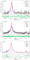 |
Fig. 2. Hβ–[O III]λλ4959,5007 spectral region in the SDSS (top panel), the X-shooter spectrum (middle panel), and the MUSE (bottom panel) spectra of PMN J0948+0022. Colors: continuum magenta – the final fit; dashed blue – the broad components of Hβ; dotted red – the narrow components of Hβ and [O III]λλ4959,5007; dotted-dashed yellow – the [O III]λλ4959,5007 blue wings, interpreted as outflows; and green – the residuals, calculated as the difference between the original data and the best-fitting model. For SDSS, the [O III]λ5007 fit is tentative; here, we applied the same model as in the other two cases, keeping in mind that we are dealing with a non-detected line. |
3.3. The resolution problem
When comparing spectra from different instruments, it is important to verify whether the line variability can be attributed to the different instrumental resolutions. X-shooter has the best spectral resolution (R = λ/Δλ ∼ 6500), followed by MUSE (R ∼ 2500), and SDSS (R ∼ 1500). We investigated the possibility that the variations in the lines were related solely to spectral resolution differences. To do so, we lowered the resolution of the X-shooter spectrum, to match those of SDSS and MUSE. Specifically, we convolved the line profiles with the line spread function expressed in terms of the R parameter (first approximation). The results are plotted in Fig. 3.
In the top-left panel of Fig. 3, we can find the difference between X-shooter and SDSS in the Hβ region, featuring a reduced resolution for the first spectrum. The difference is mainly in the central part, with a lower flux for the X-shooter case. We note that while the Hβ profile in the SDSS spectrum can be fit with a simple Lorentzian profile, this is no longer suitable for X-shooter due of the prominence of Hβ narrow component. This corresponds to the typical spectral profile of an IS (e.g., Seyfert 1943; Osterbrock & Koski 1976). We note that the flux of Hβn as measured by SDSS is more than three times that of X-shooter. Nevertheless, the low spectral resolution of SDSS hampers a complete disentangling of the different components of Hβ. Therefore, we conclude that the original classification as NLS1 was biased by the lower spectral resolution of SDSS.
In the bottom-left panel, we can see that Hβ in the MUSE case exhibits a lower flux in the central part compared to the X-shooter spectrum. From the results in Table A.1 (fitting of the unconvolved spectra), we observe that the change in the Hβn between X-shooter and MUSE is weakly significant (∼14%, ∼3σ).
In the top-right panel, we can find the same figure as the left panel, but for [O III]λ5007. Given that the measured upper limit in SDSS does not constrain the flux, it is not possible to draw important conclusions regarding its comparison with the resolution-decreased X-shooter spectrum. In the other case, we reported a significant change (> 8σ) of the core component of [O III]λ5007 (flux almost doubled), while the blue wing is more asymmetric in the MUSE profile (see Fig. 3 bottom-right panel) with the MUSE flux equal to about 71% of the X-shooter flux.
4. Results
4.1. Hβ profile
The flux of the Hβ total broad component remains stable across all the observations (variations within 1σ), as shown in Table A.1. However, the profile is changing, as indicated by the relative variation of the two sub-broad components (broad 1 and 2). Hβb1 is stable in both X-shooter and MUSE, (∼230 ⋅ 10−17 erg s−1 cm−2 in each), but shows a lower flux in SDSS (∼154 ⋅ 10−17 erg s−1 cm−2). In contrast, Hβb2 changes in all the three cases (SDSS: ∼190 ⋅ 10−17 erg s−1 cm−2; X-shooter: ∼132 ⋅ 10−17 erg s−1 cm−2; and MUSE: ∼122 ⋅ 10−17 erg s−1 cm−2). As noted in Sect. 3.2, the two broad components can be interpreted as emission from a stratified BLR (Popovic 2006). Therefore, changes in Hβb1 and Hβb2 can be interpreted as changes in the radial profile of the BLR. In addition, Cracco et al. (2016) noted that this profile is more typical of broad-line Seyfert 1 (BLS1), which strengthens our reclassification of PMN J0948+0022 as IS.
Hβn drastically decreased from SDSS to X-shooter epochs (dropping by a factor of 3.4, about 4σ), while the change from the latter to MUSE is smaller (the MUSE flux is 86% of the X-shooter value, ∼3σ), as already noted in Sect. 3.3.
From these variations, we can estimate the halving-doubling timescale, τ, by using the simple formula:
 (1)
(1)
where t1 and t2 denote the epochs of the observations (SDSS MJD 51630, X-shooter MJD 58109, and MUSE MJD 59959 ± 52, this being the middle epoch of all the MUSE observations), F(t1) and F(t2) are the fluxes, and τ represents the timescale over which the flux decreases to half (or increases to twice) its initial value.
In the Hβn case we obtain:  years for SDSS and X-shooter, and
  years for X-shooter and MUSE (see Table A.1 for the flux values).
4.2. [O III]λ5007 outflow
The first optical spectrum of PMN J0948+0022, obtained from SDSS, was analyzed by Zhou et al. (2003) who noted that the [O III]λ5007 line was not significantly detected in this spectrum. More recently, Berton et al. (2016) examined the [O III] properties of γ-ray emitters identified by Foschini et al. (2015), classifying PMN J0948+0022 among the blue outliers. These are objects with strong [O III] blueshifts exceeding 100 to several hundred km s−1 (e.g., Komossa et al. 2008). The classification by Berton et al. (2016) was driven by the presence of the prominent blue wing interpreted as an outflow, rather than the oxygen core component, which is completely buried in the noise in the SDSS spectrum, as depicted in Fig. 2. With the new X-shooter and MUSE observations, which show a significant detection of this line, we can confirm PMN J0948+0022 as a blue outlier (see Tables A.1 and A.2).
As discussed in Sect. 3, we confirmed the lack of a reliable detection of the [O III]λ5007 line in the SDSS spectrum (significance < 3σ). Consequently, we tested the best-fit model – a narrow Gaussian for the core component and a broad blueshifted Gaussian for the outflow – on the X-shooter and MUSE spectra, and applied the same model to the SDSS data. Details of the parameters are provided in Tables A.1 and A.2. The results show a blue wing with a negative velocity of < 466 km/s, (383 ± 31) km/s, and (582 ± 20) km/s, respectively in the three epochs with an increased asymmetry in the X-shooter and MUSE, as shown in the bottom-right panel of Fig. 3. This confirms the classification of PMN J0948+0022 in the blue outliers family.
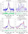 |
Fig. 3. Top panels: Comparison of the Hβ and [O III]λ5007 (left and right panels, respectively) lines observed in the SDSS−X-shooter spectra with the resolution of the latter decreased to match that of the former (SDSS in blue and X-shooter in red). Bottom panels: Same as in the top panels, but for X-shooter – MUSE with the resolution of the former reduced to match that of the latter (MUSE in blue and X-shooter in red). The left panels refer to the comparison of Hβ, while the right panels to [O III]λ5007. |
Comparing the different observations, we can calculate the halving-doubling timescale using Eq. (1). We considered only the difference between X-shooter of MUSE, because of the non-detection of [O III]λ5007 in the SDSS spectrum. The results are:  years for [O III]λ5007c, and
  years in the case of [O III]λ5007o (see Table A.1 for the flux values).
4.3. Black hole mass
To estimate MBH, we used the classical virial relation
 (2)
(2)
where f is a factor related to the geometry of the system, RBLR is the radius of the BLR, σline is the second order moment of the line profile, and G is the gravitational constant. We adopted f = (3.85 ± 1.15) as reported by Collin et al. (2006). The second order moment σline2(λ) is calculated as follows (see Eq. 3):
 (3)
(3)
where P(λ) is the profile of the selected line and λ is its wavelength.
To estimate RBLR, we employed several methods. First, we used the properties of Hβ and Eq. (4) from Greene et al. (2010), as revised by Berton et al. (2021):
 (4)
(4)
where L(Hβb) is the luminosity of the broad component of the Hβ line.
Second, we used the continuum luminosity at 5100 Å, applying Eq. (5) from Bentz et al. (2013):
 (5)
(5)
where λLλ(5100) is the continuum luminosity at 5100 Å.
Lastly, we considered an updated method that includes the iron contribution, as suggested by Du & Wang (2019), using Eq. (6):
 (6)
(6)
where R4570 = F(Fe IIλ4570)/F(Hβb), F(Fe IIλ4570) is the flux of the iron bump between 4434−4684 Å, and F(Hβb) is the flux of the broad component of Hβ.
The results are summarized in Table 2. All methods yield consistent values within the uncertainties and align with the estimates presented in Foschini et al. (2015). However, a noticeable bias is observed in the second method relative to the other two, indicating that the Bentz et al. (2013) equation may overestimate MBH. This method relies solely on the continuum luminosity, and since PMN J0948+0022 is a jetted AGN (Abdo et al. 2009b), the continuum includes contributions from both the accretion disk and the jet, which could explain the overestimation. Indeed, the jet component increases the continuum flux, leading to an overestimation of the BLR radius.
MBH, REdd, and Lbol along with their associated uncertainties for SDSS, X-shooter, and MUSE spectra of PMN J0948+0022.
It is also worth noting that the method incorporating the iron contribution (Eq. 6) may be affected by systematic uncertainties due the complexities of fitting and subtracting the iron emission. For this reason, we adopted the black hole mass estimate obtained from the first method (Eq. 4) by Greene et al. (2010) for the subsequent analysis. We calculated the weighted average between the three results (SDSS, X-shooter, and MUSE), obtaining log(MBH) = (7.76 ± 0.12) M⊙ (last row of Table 2).
4.4. Eddington ratio
Given the MBH parameter, we can derive REdd using Eq. (7):
 (7)
(7)
where Lbol denotes the bolometric luminosity, which primarily reflects the accretion disk emission, and ṁ is the accretion parameter (the last equality is true if the efficiency η is constant). The most common method for estimating the disk luminosity is through the equation provided by Kaspi et al. (2000), which relates Lbol to the continuum luminosity at 5100 Å:
 (8)
(8)
The continuum luminosity can be directly measured from the spectrum and substituted into the above equation. Alternatively, we can invert Eqs. (5) and (6) to calculate the continuum luminosity from RBLR obtained using Eq. (4). This latter approach derives the continuum based on line properties, specifically as a function of L(Hβb). The inverted forms of Eqs. (5) and (6) are
![Mathematical equation: $$ \begin{aligned} {\log }\frac{\lambda L_{{\lambda }}(5100)}{10^{44}\,\mathrm{erg/s}}&= \left[\log \left(\frac{R_{\mathrm{BLR} }}{1\,\mathrm{lt-day}}\right) - (1.53 \pm 0.03)\right] \cdot \frac{1}{(0.53 \pm 0.03)}, \end{aligned} $$](/articles/aa/full_html/2025/06/aa52421-24/aa52421-24-eq13.gif) (9)
(9)
![Mathematical equation: $$ \begin{aligned} {\log }\frac{\lambda L_{{\lambda }}(5100)}{10^{44}\,\mathrm{erg/s}}&= \left[\log \left(\frac{R_{\mathrm{BLR} }}{1\,\mathrm{lt-day}}\right) - (1.65 \pm 0.06)\right.\nonumber \\&\qquad \left. + (0.35 \pm 0.08) \times R_{4570} \right] \cdot \frac{1}{(0.45 \pm 0.03)}\cdot \end{aligned} $$](/articles/aa/full_html/2025/06/aa52421-24/aa52421-24-eq14.gif) (10)
(10)
All three methods are affected by different sources of bias. Directly using Eq. (8) encounters similar issues as Eq. (5), as it relies on continuum measurements from the spectrum. As discussed in Sect. 4.3, for jetted sources, the continuum includes contributions from both the accretion disk and the jet, leading to contamination in the measurements. Conversely, the other two methods derive the continuum from line properties, in particular Hβ. Equation (10) is influenced by the iron fitting process, making the second method (inverting Eq. 5 into Eq. 9 and using RBLR from Eq. 4) a less biased approach in our specific scenario.
The results are shown in Table 2. It is evident from the table that the second method yields the most consistent results, whereas the other two methods exhibit more variability, likely influenced by jet activity. Consequently, we used the value calculated with Eq. (9) (central section, last column of Table 2) as the reference for λLλ(5100). The weighted average between the X-shooter and MUSE values of the second method the reference value for the discussion (REdd = 0.21 ± 0.06), as shown in the last row of Table 2.
4.5. Geometry of the system
We derived the key geometrical parameters necessary to construct a schematic representation of the AGN. These include the sublimation radius (Rsub), which represents the boundary between the BLR and the dusty torus; the outer radius (Rout), the outer boundary of the dusty torus; and the maximum extent of the NLR (RNLR). These quantities were computed using the following relations from Elitzur (2008) and Fischer et al. (2018):
 (11)
(11)
 (12)
(12)
![Mathematical equation: $$ \begin{aligned} R_{\mathrm{NLR} }&= 10^{-18.41 + 0.52 \cdot {\log }\,L_{\rm [O\,III] }}. \end{aligned} $$](/articles/aa/full_html/2025/06/aa52421-24/aa52421-24-eq17.gif) (13)
(13)
All these quantities are functions of Lbol (reported in Table 2) or of the [O III]λ5007 luminosity L[O III]. Results are reported in Table 3 in parsecs. There is general agreement in the Rsub and Rout parameters, while the NLR in the SDSS case appears to be more extended. It is important to note that the NLR size is determined from the [O III]λ5007 properties (see Eq. 13), and in the SDSS spectrum this line was not significantly detected, providing only an upper limit.
Geometric parameters for PMN J0948+0022.
5. Discussion
Variations in optical line properties are generally attributed to changes in the accretion activity of the disk. However, this explanation only partially applies to the case of PMN J0948+0022. The REdd parameter, reported in Table 2 and calculated using Eq. (9), remains consistent across different observations. Spectral variations driven by accretion activity typically emerge first in the BLR (after ∼46 days, in our case) and propagate to the NLR over longer timescales (∼2700 years, for PMN J0948+0022). In our case, the flux of Hβb remains stable over time, although we observed changes in Hβb1 and Hβb2, which suggest an adjustment of the stratification. Conversely, we observed changes in the Hβn and [O III]λ5007.
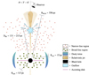 |
Fig. 4. Schematic representation of PMN J0948+0022. The scheme is not to scale. |
As noted in Sect. 3.3, the better spectral resolution of X-shooter and MUSE, requires a change in the Hβ line profile from a Lorentzian to a combination of three Gaussians, which is typical of ISs. This type of reclassification is not unprecedented. For instance, SDSS J211852.96−073227.5 and SDSS J164100.10+345452.7 were initially classified as NLS1, and later reclassified as IS following new observations (Järvelä et al. 2020; Crepaldi et al. 2025). However, as we will show, PMN J0948+0022 is a different case.
According to the UM, IS are viewed at large angles, and consequently the composite profile is due to partial obscuration. This is the case of SDSS J164100.10+345452.7 – reclassified as IS by Crepaldi et al. (2025) – which displays intrinsic obscuration in X-rays (Romano et al. 2023). In contrast, many authors (Foschini et al. 2015; Bhattacharyya et al. 2014; D’Ammando et al. 2014; Berton et al. 2019) found that PMN J0948+0022 does not show any evidence of intrinsic obscuration in X-rays.
The optical spectra analyzed in the present work also support the absence of intrinsic absorption. In particular, the detection of prominent iron multiplets (R4570 ≳ 1) – thought to originate in the innermost regions of the NLR, close to the accretion disk and within the obscuring torus (Dong et al. 2010) – further supports this scenario. While the Fe II bump strength shows some dependence on inclination, this effect is considered secondary (Śniegowska et al. 2023; Panda et al. 2020) and should be interpreted as such.
Another point refers to the effect of the obscuration on the FWHM of the broad lines. In this case, we would expect some difference between Hβ at 4861 Å and Hα at 6563 Å, since the latter is in the red part of the spectrum. However, we find consistent values within 2σ: FWHM(Hβb) = 1520 ± 31 km s−1 and FWHM(Hαb) = 1466 ± 20 km s−1.
In addition, we know the viewing angle of the relativistic jet to be about 3° −6° (Abdo et al. 2009b; Foschini et al. 2012; Doi et al. 2019). Since it is known that there is a strong correlation between the jet and the NLR-bicone axes, but no correlation with the host-galaxy axis (Schmitt et al. 2003a,b; Fischer et al. 2013, 2014), the small jet viewing angle confirms that the object is observed almost face-on. There are cases of misalignment between the AGN and the host galaxy (Circosta et al. 2019; Malizia et al. 2020), see also the case of NGC 5506 described in (Nagar et al. 2002; Fischer et al. 2013, 2014), but – again – in such a case we should observe an additional absorption at X-rays, which is not the case. Furthermore, such a misalignment would likely be a result of a recent merger, which is ruled out by Olguín-Iglesias et al. (2020).
If no obscuration in PMN J0948+0022 is affecting the spectral lines, another mechanism must be considered to explain the observed variations. A starting point is to focus on the changes in the Hβn and [O III] lines. Specifically, the changes of Hβn on timescales of ∼10−27 years, much smaller than those expected from the NLR (∼2700 years) point to a mechanism different from the AGN ionization. Given the presence of a relativistic jet, it is straightforward to study the interaction between the jet and the NLR (e.g., Rawlings & Saunders 1991; Mullaney et al. 2013; Berton et al. 2016; Meenakshi et al. 2022; Escott et al. 2025).
By studying the radio morphology and emission of PMN J0948+0022, Doi et al. (2019) found that the relativistic jet changed its shape, from parabolic to conic, in the NLR (distance from the center 100−430 pc). This process is due to deceleration as the jet is converting part of its kinetic energy into internal energy. The observed changes in the [O III]λ5007 line suggest that this internal energy is then dissipated in the NLR. To prove this hypothesis, we can calculate the location where this occurs, by using the timescales obtained in Sect. 4.2. The relationship between the timescale and the dimension of the emitting region rIR is given by
 (14)
(14)
where c is the speed of light, z is the redshift,  years, and δ is the Doppler factor. After four years of observations of PMN J0948+0022, Foschini et al. (2012) reported changes of the bulk Lorentz factor (Γ) between 11 and 16. By assuming a viewing angle of 3°, it results δ = 16.5 − 18.8. Given the self-similarity of the jet and assuming a typical scaling factor of 0.1, then the distance from the central BH is
 (15)
(15)
Homan et al. (2021) reported δ = 47 on the basis of Very Long Baseline Interferometer (VLBI) radio observations at 15 GHz. By assuming this value, and τ = 4.8 years, DIR ∼ 435 pc. All these values are consistent with the distance found by Doi et al. (2019) and thus strengthens our hypothesis that we observe, at optical wavelengths, the transfer of the jet internal energy to the NLR. Since the [O III]λ5007c increases from X-shooter to MUSE observations, we expect a corresponding decrease of the jet activity. This is precisely what we observe at high-energy in the γ−ray (0.1−100 GeV) light curve from Fermi Large Area Telescope (LAT)9, displayed in Fig. 5. The binning is one month, to enhance the long-term activity periods. Since high-energy γ-rays are a clear product of the relativistic jet, it is evident from this plot that, after a significant activity period, the source has been in a quiet state since 2020. Specifically, the activity showed an notable peak around 2017−2018. Comparing the periods in which the X-shooter and MUSE observations were carried out, we note an almost order of magnitude difference in the γ photon flux (∼2 ⋅ 10−7 ph cm−2 s−1 in August 2017 versus ∼6 ⋅ 10−8 ph cm−2 s−1 in January 2023). For the SDSS period, we do not have any data points because the Fermi satellite was not operating at that time.
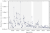 |
Fig. 5. Fermi light curve for PMN J0948+0022 with a data binning of one month. We highlighted the two periods that coincide with the X-shooter and MUSE observations. The highlighted peak was observed on August 2, 2017. The quiet phase began on April 18, 2020, and is still ongoing. |
A similar, but opposite, effect is also visible in the [O III]λ5007o component, which displays: a flux decrease, an increase in its velocity (Δv ∼ 200 km s−1) together with a strengthening of the asymmetry (see Fig. 3). All these variations occurred in a timescale (∼10 years), which is consistent with that of Hβn one (τ ∼ 10 − 27).
To summarize, we propose the following scenario: according to radio observations (Doi et al. 2019), at a distance of about 100−430 pc from the central BH the jet decelerates, changes its shape from parabolic to conical, and converts part of its kinetic energy into internal energy. From the optical observations, presented in this work, we suggest that the jet internal energy is transferred to the NLR (increase of [O III]λ5007c flux), which generates an outflow propagating along the NLR and affecting Hβn, see Fig. 4.
6. Conclusions
We analyzed three optical spectra of PMN J0948+0022 taken at different epochs, specifically in 2000 (SDSS), 2017 (X-shooter), and 2022−2023 (MUSE, composition). The source exhibits multiwavelength variability, but we focused on the Hβ and [O III]λ5007 spectral lines. We tested the robustness of the variations in these lines by reducing the spectral resolution of the X-shooter spectrum to match that of the SDSS and MUSE spectra. We find the following:
-
Despite being initially classified as an NLS1 based on the SDSS spectrum (Zhou et al. 2003), the higher resolution of X-shooter and MUSE supports its reclassification as an IS (see Sect. 3.3); however, the Hβ composite profile is not due to a geometrical effect of partial obscuration, but rather to the interaction of the relativistic jet with the NLR.
-
Although the total flux of the broad component of Hβ is stable during all the observations (variations within 1σ), there are changes in the two subcomponents Hβb1 and Hβb2, which imply a stratification of the BLR.
-
We observe significant variation in the Hβn (an ∼4σ variation in flux between SDSS and X-shooter, and an ∼3σ between X-shooter and MUSE) as well as in the [O III]λ5007 line flux and asymmetry (a variation > 8σ in flux between X-shooter and MUSE), which we interpret as the interaction of the relativistic jet with the NLR, confirming the results of Doi et al. (2019) based on radio observations. The relativistic jet decelerates in the NLR (131−215 pc from the central BH), changes its shape from parabolic to conic, and converts part of its kinetic energy into internal energy. This internal energy then dissipates in the NLR, generating an outflow revealed by the blue wing in the [O III] line.
-
Based on these new high-quality spectra and considering the lack of additional obscuration, we recalculated MBH = 107.76 ± 0.12 M⊙ and REdd = (0.21 ± 0.06).
Lastly, we emphasize the importance of high-spectral-resolution optical spectroscopy, to be performed with instruments such as X-shooter or its successor Son of X-shooter (SOXS), in order to gain deeper insight into the jet-NLR interaction. This approach would allow for a better understanding of the possible connection between high-energy processes – such as the γ-ray emission from AGNs – and their optical counterpart.
Sloan Digital Sky Survey-DR9 (Ahn et al. 2012).
Acknowledgments
The authors thank Dr. N. Winkel for the fruitful discussion during the MUSE-10yrs workshop (Garching bei München, November 18–22). The authors thank the referee for the detailed and helpful review of the manuscript, which was significantly improved by the received comments. G.V. acknowledges support from the European Union (ERC, WINGS, 101040227). Based on observations collected at the European Southern Observatory under ESO programmes 099.B-0785(A) and 110.23WR.001. Funding for the Sloan Digital Sky Survey IV has been provided by the Alfred P. Sloan Foundation, the U.S. Department of Energy Office of Science, and the Participating Institutions. SDSS acknowledges support and resources from the Center for High-Performance Computing at the University of Utah. The SDSS website is www.sdss4.org. SDSS is managed by the Astrophysical Research Consortium for the Participating Institutions of the SDSS Collaboration including the Brazilian Participation Group, the Carnegie Institution for Science, Carnegie Mellon University, Center for Astrophysics | Harvard & Smithsonian (CfA), the Chilean Participation Group, the French Participation Group, Instituto de Astrofísica de Canarias, The Johns Hopkins University, Kavli Institute for the Physics and Mathematics of the Universe (IPMU)/University of Tokyo, the Korean Participation Group, Lawrence Berkeley National Laboratory, Leibniz Institut für Astrophysik Potsdam (AIP), Max-Planck-Institut für Astronomie (MPIA Heidelberg), Max-Planck-Institut für Astrophysik (MPA Garching), Max-Planck-Institut für Extraterrestrische Physik (MPE), National Astronomical Observatories of China, New Mexico State University, New York University, University of Notre Dame, Observatório Nacional/MCTI, The Ohio State University, Pennsylvania State University, Shanghai Astronomical Observatory, United Kingdom Participation Group, Universidad Nacional Autónoma de México, University of Arizona, University of Colorado Boulder, University of Oxford, University of Portsmouth, University of Utah, University of Virginia, University of Washington, University of Wisconsin, Vanderbilt University, and Yale University. This research has made use of the NASA/IPAC Extragalactic Database (NED), which is operated by the Jet Propulsion Laboratory, California Institute of Technology, under contract with the National Aeronautics and Space Administration.
References
- Abazajian, K. N., Adelman-McCarthy, J. K., Agüeros, M. A., et al. 2009, ApJS, 182, 543 [Google Scholar]
- Abdo, A. A., Ackermann, M., Ajello, M., et al. 2009a, ApJ, 707, 727 [NASA ADS] [CrossRef] [Google Scholar]
- Abdo, A. A., Ackermann, M., Ajello, M., et al. 2009b, ApJ, 707, L142 [NASA ADS] [CrossRef] [Google Scholar]
- Ahn, C. P., Alexandroff, R., Allende Prieto, C., et al. 2012, ApJS, 203, 21 [Google Scholar]
- Ahumada, R., Allende Prieto, C., Almeida, A., et al. 2020, ApJS, 249, 3 [NASA ADS] [CrossRef] [Google Scholar]
- Alam, S., Albareti, F. D., Allende Prieto, C., et al. 2015, ApJS, 219, 12 [Google Scholar]
- Angelakis, E., Fuhrmann, L., Marchili, N., et al. 2015, A&A, 575, A55 [NASA ADS] [CrossRef] [EDP Sciences] [Google Scholar]
- Antonucci, R. 1993, ARA&A, 31, 473 [Google Scholar]
- Baldwin, J. A., Phillips, M. M., & Terlevich, R. 1981, PASP, 93, 5 [Google Scholar]
- Bentz, M. C., Denney, K. D., Grier, C. J., et al. 2013, ApJ, 767, 149 [Google Scholar]
- Berton, M., Foschini, L., Ciroi, S., et al. 2016, A&A, 591, A88 [NASA ADS] [CrossRef] [EDP Sciences] [Google Scholar]
- Berton, M., Foschini, L., Caccianiga, A., et al. 2017, Front. Astron. Space Sci., 4, 8 [NASA ADS] [CrossRef] [Google Scholar]
- Berton, M., Braito, V., Mathur, S., et al. 2019, A&A, 632, A120 [NASA ADS] [CrossRef] [EDP Sciences] [Google Scholar]
- Berton, M., Peluso, G., Marziani, P., et al. 2021, A&A, 654, A125 [NASA ADS] [CrossRef] [EDP Sciences] [Google Scholar]
- Bhattacharyya, S., Bhatt, H., Bhatt, N., & Singh, K. K. 2014, MNRAS, 440, 106 [Google Scholar]
- Blandford, R., Meier, D., & Readhead, A. 2019, ARA&A, 57, 467 [NASA ADS] [CrossRef] [Google Scholar]
- Circosta, C., Vignali, C., Gilli, R., et al. 2019, A&A, 623, A172 [NASA ADS] [CrossRef] [EDP Sciences] [Google Scholar]
- Collin, S., Kawaguchi, T., Peterson, B. M., & Vestergaard, M. 2006, A&A, 456, 75 [NASA ADS] [CrossRef] [EDP Sciences] [Google Scholar]
- Comparat, J., Kneib, J.-P., Bacon, R., et al. 2013, A&A, 559, A18 [NASA ADS] [CrossRef] [EDP Sciences] [Google Scholar]
- Cracco, V., Ciroi, S., Berton, M., et al. 2016, MNRAS, 462, 1256 [NASA ADS] [CrossRef] [Google Scholar]
- Crepaldi, L., Berton, M., Dalla Barba, B., et al. 2025, A&A, 696, A74 [NASA ADS] [CrossRef] [EDP Sciences] [Google Scholar]
- D’Ammando, F., Larsson, J., Orienti, M., et al. 2014, MNRAS, 438, 3521 [Google Scholar]
- D’Ammando, F., Orienti, M., Finke, J., et al. 2015, MNRAS, 446, 2456 [Google Scholar]
- Dimitrijević, M. S., Kovačević, J., Popović, L. Č., Dačić, M., & Ilić, D. 2007, AIP Conf. Ser., 895, 313 [CrossRef] [Google Scholar]
- Doi, A., Nagai, H., Asada, K., et al. 2006, PASJ, 58, 829 [NASA ADS] [Google Scholar]
- Doi, A., Nagira, H., Kawakatu, N., et al. 2012, ApJ, 760, 41 [NASA ADS] [CrossRef] [Google Scholar]
- Doi, A., Nakahara, S., Nakamura, M., et al. 2019, MNRAS, 487, 640 [NASA ADS] [CrossRef] [Google Scholar]
- Dojčinović, I., Kovačević-Dojčinović, J., & Popović, L. Č. 2023, Adv. Space Res., 71, 1219 [CrossRef] [Google Scholar]
- Donato, D. 2010, ATel, 2733, 1 [Google Scholar]
- Dong, X.-B., Ho, L. C., Wang, J.-G., et al. 2010, ApJ, 721, L143 [NASA ADS] [CrossRef] [Google Scholar]
- Drinkwater, M. J., Byrne, Z. J., Blake, C., et al. 2018, MNRAS, 474, 4151 [Google Scholar]
- Du, P., & Wang, J.-M. 2019, ApJ, 886, 42 [NASA ADS] [CrossRef] [Google Scholar]
- Duncan, K. J. 2022, MNRAS, 512, 3662 [NASA ADS] [CrossRef] [Google Scholar]
- Elitzur, M. 2008, New Astron. Rev., 52, 274 [CrossRef] [Google Scholar]
- Escott, E. L., Morabito, L. K., Scholtz, J., et al. 2025, MNRAS, 536, 1166 [Google Scholar]
- Foschini, L., Fermi/Lat Collaboration, Ghisellini, G., et al. 2010, ASP Conf. Ser., 427, 243 [NASA ADS] [Google Scholar]
- Fischer, T. C., Crenshaw, D. M., Kraemer, S. B., & Schmitt, H. R. 2013, ApJS, 209, 1 [Google Scholar]
- Fischer, T. C., Crenshaw, D. M., Kraemer, S. B., Schmitt, H. R., & Turner, T. J. 2014, ApJ, 785, 25 [CrossRef] [Google Scholar]
- Fischer, T. C., Kraemer, S. B., Schmitt, H. R., et al. 2018, ApJ, 856, 102 [Google Scholar]
- Foschini, L. 2020, Universe, 6, 136 [NASA ADS] [CrossRef] [Google Scholar]
- Foschini, L., Ghisellini, G., Kovalev, Y. Y., et al. 2011, MNRAS, 413, 1671 [Google Scholar]
- Foschini, L., Angelakis, E., Fuhrmann, L., et al. 2012, A&A, 548, A106 [NASA ADS] [CrossRef] [EDP Sciences] [Google Scholar]
- Foschini, L., Berton, M., Caccianiga, A., et al. 2015, A&A, 575, A13 [NASA ADS] [CrossRef] [EDP Sciences] [Google Scholar]
- Foschini, L., Lister, M. L., Andernach, H., et al. 2022, Universe, 8, 587 [NASA ADS] [CrossRef] [Google Scholar]
- Fossati, G., Maraschi, L., Celotti, A., Comastri, A., & Ghisellini, G. 1998, MNRAS, 299, 433 [Google Scholar]
- Ghisellini, G., Celotti, A., Fossati, G., Maraschi, L., & Comastri, A. 1998, MNRAS, 301, 451 [NASA ADS] [CrossRef] [Google Scholar]
- Giroletti, M., Paragi, Z., Bignall, H., et al. 2011, A&A, 528, L11 [NASA ADS] [CrossRef] [EDP Sciences] [Google Scholar]
- Goodrich, R. W. 1989, ApJ, 342, 224 [Google Scholar]
- Greene, J. E., Hood, C. E., Barth, A. J., et al. 2010, ApJ, 723, 409 [NASA ADS] [CrossRef] [Google Scholar]
- Homan, D. C., Cohen, M. H., Hovatta, T., et al. 2021, ApJ, 923, 67 [NASA ADS] [CrossRef] [Google Scholar]
- Ilić, D., Oknyansky, V., Popović, L. Č., et al. 2020, A&A, 638, A13 [NASA ADS] [CrossRef] [EDP Sciences] [Google Scholar]
- Ilić, D., Rakić, N., & Popović, L. Č. 2023, ApJS, 267, 19 [CrossRef] [Google Scholar]
- Järvelä, E., Berton, M., Ciroi, S., et al. 2020, A&A, 636, L12 [NASA ADS] [CrossRef] [EDP Sciences] [Google Scholar]
- Kaspi, S., Smith, P. S., Netzer, H., et al. 2000, ApJ, 533, 631 [Google Scholar]
- Kauffmann, G., Heckman, T. M., Tremonti, C., et al. 2003, MNRAS, 346, 1055 [Google Scholar]
- Keel, W. C. 1980, AJ, 85, 198 [Google Scholar]
- Kewley, L. J., Groves, B., Kauffmann, G., & Heckman, T. 2006, MNRAS, 372, 961 [Google Scholar]
- Komossa, S., Xu, D., Zhou, H., Storchi-Bergmann, T., & Binette, L. 2008, ApJ, 680, 926 [NASA ADS] [CrossRef] [Google Scholar]
- Lähteenmäki, A., Järvelä, E., Hovatta, T., et al. 2017, A&A, 603, A100 [NASA ADS] [CrossRef] [EDP Sciences] [Google Scholar]
- Lister, M. L., Aller, M. F., Aller, H. D., et al. 2016, AJ, 152, 12 [NASA ADS] [CrossRef] [Google Scholar]
- Liu, H., Wang, J., Mao, Y., & Wei, J. 2010, ApJ, 715, L113 [NASA ADS] [CrossRef] [Google Scholar]
- Malizia, A., Bassani, L., Stephen, J. B., Bazzano, A., & Ubertini, P. 2020, A&A, 639, A5 [NASA ADS] [CrossRef] [EDP Sciences] [Google Scholar]
- Mao, L. 2021, Res. Notes Am. Astron. Soc., 5, 109 [Google Scholar]
- Mathur, S. 2000, MNRAS, 314, L17 [NASA ADS] [CrossRef] [Google Scholar]
- Meenakshi, M., Mukherjee, D., Wagner, A. Y., et al. 2022, MNRAS, 516, 766 [NASA ADS] [CrossRef] [Google Scholar]
- Mullaney, J. R., Alexander, D. M., Fine, S., et al. 2013, MNRAS, 433, 622 [Google Scholar]
- Nagar, N. M., Oliva, E., Marconi, A., & Maiolino, R. 2002, A&A, 391, L21 [NASA ADS] [CrossRef] [EDP Sciences] [Google Scholar]
- Ojha, V., Chand, H., & Gopal-Krishna 2021, MNRAS, 501, 4110 [Google Scholar]
- Ojha, V., Jha, V. K., Chand, H., & Singh, V. 2022, MNRAS, 514, 5607 [Google Scholar]
- Olguín-Iglesias, A., Kotilainen, J., & Chavushyan, V. 2020, MNRAS, 492, 1450 [Google Scholar]
- Osterbrock, D. E., & Ferland, G. J. 2006, Astrophysics of Gaseous Nebulae and Active Galactic Nuclei (Sausalito: University Science Books) [Google Scholar]
- Osterbrock, D. E., & Koski, A. T. 1976, MNRAS, 176, 61P [NASA ADS] [CrossRef] [Google Scholar]
- Osterbrock, D. E., & Pogge, R. W. 1985, ApJ, 297, 166 [Google Scholar]
- Panda, S., Marziani, P., & Czerny, B. 2020, Contrib. Astron. Obs. Skaln. Pleso, 50, 293 [Google Scholar]
- Popovic, L. C. 2006, Serb. Astron. J., 173, 1 [Google Scholar]
- Pradhan, A. K., Montenegro, M., Nahar, S. N., & Eissner, W. 2006, MNRAS, 366, L6 [NASA ADS] [CrossRef] [Google Scholar]
- Rakić, N. 2022, MNRAS, 516, 1624 [CrossRef] [Google Scholar]
- Rawlings, S., & Saunders, R. 1991, Nature, 349, 138 [NASA ADS] [CrossRef] [Google Scholar]
- Riess, A. G., Yuan, W., Macri, L. M., et al. 2022, ApJ, 934, L7 [NASA ADS] [CrossRef] [Google Scholar]
- Romano, P., Lähteenmäki, A., Vercellone, S., et al. 2023, A&A, 673, A85 [NASA ADS] [CrossRef] [EDP Sciences] [Google Scholar]
- Schmitt, H. R., Donley, J. L., Antonucci, R. R. J., et al. 2003a, ApJ, 597, 768 [NASA ADS] [CrossRef] [Google Scholar]
- Schmitt, H. R., Donley, J. L., Antonucci, R. R. J., Hutchings, J. B., & Kinney, A. L. 2003b, ApJS, 148, 327 [NASA ADS] [CrossRef] [Google Scholar]
- Schönebeck, F., Puzia, T. H., Pasquali, A., et al. 2014, A&A, 572, A13 [NASA ADS] [CrossRef] [EDP Sciences] [Google Scholar]
- Seyfert, C. K. 1943, ApJ, 97, 28 [NASA ADS] [CrossRef] [Google Scholar]
- Śniegowska, M., Panda, S., Czerny, B., et al. 2023, A&A, 678, A63 [NASA ADS] [CrossRef] [EDP Sciences] [Google Scholar]
- Urry, C. M., & Padovani, P. 1995, PASP, 107, 803 [NASA ADS] [CrossRef] [Google Scholar]
- Varglund, I., Järvelä, E., Ciroi, S., et al. 2023, A&A, 679, A32 [NASA ADS] [CrossRef] [EDP Sciences] [Google Scholar]
- Veilleux, S., & Osterbrock, D. E. 1987, ApJS, 63, 295 [Google Scholar]
- Weilbacher, P. M., Palsa, R., Streicher, O., et al. 2020, A&A, 641, A28 [NASA ADS] [CrossRef] [EDP Sciences] [Google Scholar]
- Williams, R. J., Pogge, R. W., & Mathur, S. 2002, AJ, 124, 3042 [CrossRef] [Google Scholar]
- Xin, Y.-X., Xiong, D.-R., Bai, J.-M., et al. 2022, RAA, 22, 075001 [Google Scholar]
- Yao, S., & Komossa, S. 2023, MNRAS, 523, 441 [Google Scholar]
- Zhang, J., Zhang, H.-M., Zhu, Y.-K., et al. 2017, ApJ, 849, 42 [Google Scholar]
- Zhou, H.-Y., Wang, T.-G., Dong, X.-B., Zhou, Y.-Y., & Li, C. 2003, ApJ, 584, 147 [NASA ADS] [CrossRef] [Google Scholar]
Appendix A: Fitting parameters
In this section we present the fitting parameters of the different lines in the SDSS, X-shooter, and MUSE spectra (see Table A.2).
By comparing the flux of the [O II]λλ3726,3729 lines, we obtain a ratio of approximately 1.4–1.2. Some authors (Pradhan et al. 2006; Comparat et al. 2013) have found a typical range of 1.5 to 0.35 for this ratio, where the limit values correspond to low (→0) and high (→∞) electron densities, respectively. From our result, we can infer that the [O II] gas is associated with an extremely low electron density.
Furthermore, due to the X-shooter spectral coverage, it is possible to obtain two additional properties of the system from Hα and [N II]λ6583: the Seyfert type (discussed in Sects. 3.3 and 4.1) and the classification from the Baldwin, Phillips, and Terlevich-Veilleux & Osterbrock (BPT-VO) diagram (Baldwin et al. 1981; Veilleux & Osterbrock 1987). The BPT-VO diagram relates Hα and Hβ in their narrow components, to [O III]λ5007 and [N II]λ6583. In this case, followingKauffmann et al. 2003; Kewley et al. 2006 classifications, PMN J0948+0022 is an AGN that lies close to the separation between Seyfert and Low-Ionization Nuclear Emission-line Regions. The obtained ratios are: log([N II]/Hα) = (-0.38±0.05) and log([O III]/Hβ) = (-0.01±0.12).
Most important identified lines.
Fitting parameters for the main spectral lines and the observed redshifts (zobs) for those lines identified at least at 5σ.
Appendix B: Telluric contamination in Hβ
The original shape of Hβ is affected by significant telluric absorption in the blue part (see Fig. B.1). To correct for this contribution, we assumed a symmetric shape for Hβ, based on that of Hα. Consequently, we mirrored the right side of the line onto the left side and added random noise proportional to what was observed in the 5050–5150 Å range. The entire procedure was performed using IRAF and specific Python codes.
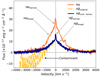 |
Fig. B.1. Comparison between Hβ (in blue for the corrected profile, and in dotted-yellow for the contaminated one) and Hα (in orange) in the X-shooter spectrum. The gray arrows refer to the broad and narrow components of Hβ and Hα. The black arrow stresses the position of the telluric absorption. |
Appendix C: Other sources in the MUSE FoV
As an IFS, MUSE produces data cubes that can be separated in two components: one for the two spatial directions (x,y) (see for example the FoV of PMN J0948+0022 in Fig. C.1), and one spectral direction (z) for each pixel. In Table C.1 we present the first measurement of the spectroscopic redshift of the sources in the MUSE FoV of PMN J0948+0022. The selection of the sources was made applying a filter to the original data cube, limiting those sources with a flux smaller than 4 × 10⁻²⁰ erg s−1 cm−2. This threshold corresponds to ∼2 times the noise level, calculated in an empty region of the image (top-left part of Fig. C.1). All the objects that we present are galaxies, except for [VV2006] J094855.7+002238. It is also important to stress the presence of a possible artifact, highlighted by the yellow circle in Fig. C.1. In this position none of the public catalogs present a source, so we classified it as an instrumental effect. The resulting redshift is the weighted average of the redshifts for all the identified lines in the corresponding spectra.
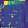 |
Fig. C.1. MUSE WFM-NOAO FoV (1x1 arcmin2) of PMN J0948+0022 (at the center). The MUSE scale is of 0.2 arcsec/pixel. Combined with the scale of PMN J0948+0022 of s = 6.31 kpc/arcsec, this yields ∼ 1.26 kpc/pixel for the central source. We averaged the z-axis (spectral axis) to enhance the flux for each pixel of the image. The white circles indicate the sources for which we measured the spectroscopic redshifts. The numbers correspond to those listed in the first column of Table C.1. |
Objects in the MUSE FoV.
All Tables
MBH, REdd, and Lbol along with their associated uncertainties for SDSS, X-shooter, and MUSE spectra of PMN J0948+0022.
Fitting parameters for the main spectral lines and the observed redshifts (zobs) for those lines identified at least at 5σ.
All Figures
|
Fig. 1. Top: Three redshift-corrected spectra in the visible range. Bottom: Three redshift-corrected spectra, with the continuum and iron lines subtracted shown. The X-shooter spectrum is composed of three sections, but here we report only the one useful for the comparison with the SDSS and MUSE spectra. In both panels, we present the SDSS spectrum in light blue, the X-shooter spectrum in blue, and the MUSE spectrum in magenta. The vertical lines correspond to the identified optical lines with a significance > 5σ in all the spectra, except for [O III]λ5007, which was included even though it was not detected in the SDSS spectrum. |
| In the text | |
|
Fig. 2. Hβ–[O III]λλ4959,5007 spectral region in the SDSS (top panel), the X-shooter spectrum (middle panel), and the MUSE (bottom panel) spectra of PMN J0948+0022. Colors: continuum magenta – the final fit; dashed blue – the broad components of Hβ; dotted red – the narrow components of Hβ and [O III]λλ4959,5007; dotted-dashed yellow – the [O III]λλ4959,5007 blue wings, interpreted as outflows; and green – the residuals, calculated as the difference between the original data and the best-fitting model. For SDSS, the [O III]λ5007 fit is tentative; here, we applied the same model as in the other two cases, keeping in mind that we are dealing with a non-detected line. |
| In the text | |
|
Fig. 3. Top panels: Comparison of the Hβ and [O III]λ5007 (left and right panels, respectively) lines observed in the SDSS−X-shooter spectra with the resolution of the latter decreased to match that of the former (SDSS in blue and X-shooter in red). Bottom panels: Same as in the top panels, but for X-shooter – MUSE with the resolution of the former reduced to match that of the latter (MUSE in blue and X-shooter in red). The left panels refer to the comparison of Hβ, while the right panels to [O III]λ5007. |
| In the text | |
|
Fig. 4. Schematic representation of PMN J0948+0022. The scheme is not to scale. |
| In the text | |
|
Fig. 5. Fermi light curve for PMN J0948+0022 with a data binning of one month. We highlighted the two periods that coincide with the X-shooter and MUSE observations. The highlighted peak was observed on August 2, 2017. The quiet phase began on April 18, 2020, and is still ongoing. |
| In the text | |
|
Fig. B.1. Comparison between Hβ (in blue for the corrected profile, and in dotted-yellow for the contaminated one) and Hα (in orange) in the X-shooter spectrum. The gray arrows refer to the broad and narrow components of Hβ and Hα. The black arrow stresses the position of the telluric absorption. |
| In the text | |
|
Fig. C.1. MUSE WFM-NOAO FoV (1x1 arcmin2) of PMN J0948+0022 (at the center). The MUSE scale is of 0.2 arcsec/pixel. Combined with the scale of PMN J0948+0022 of s = 6.31 kpc/arcsec, this yields ∼ 1.26 kpc/pixel for the central source. We averaged the z-axis (spectral axis) to enhance the flux for each pixel of the image. The white circles indicate the sources for which we measured the spectroscopic redshifts. The numbers correspond to those listed in the first column of Table C.1. |
| In the text | |
Current usage metrics show cumulative count of Article Views (full-text article views including HTML views, PDF and ePub downloads, according to the available data) and Abstracts Views on Vision4Press platform.
Data correspond to usage on the plateform after 2015. The current usage metrics is available 48-96 hours after online publication and is updated daily on week days.
Initial download of the metrics may take a while.