| Issue |
A&A
Volume 673, May 2023
|
|
|---|---|---|
| Article Number | A57 | |
| Number of page(s) | 13 | |
| Section | The Sun and the Heliosphere | |
| DOI | https://doi.org/10.1051/0004-6361/202245825 | |
| Published online | 04 May 2023 | |
Statistical study of type III bursts and associated HXR emissions
1
LESIA, Observatoire de Paris, Université PSL, CNRS, Sorbonne Université, Université Paris Cité, 5 place Jules Janssen, 92195 Meudon, France
e-mail: This email address is being protected from spambots. You need JavaScript enabled to view it.
2
Observatoire Radioastronomique de Nançay, Observatoire de Paris, PSL Research University, CNRS, Univ. Orléans, route de Souesmes 18330 Nançay, France
Received:
30
December
2022
Accepted:
24
March
2023
Abstract
Context. Flare-accelerated electrons may produce closely temporarily related hard X-ray (HXR) emission while interacting with the dense solar atmosphere and radio type III bursts when propagating from the low corona to the interplanetary medium. The link between these emissions has been studied in previous studies. We present here new results on the correlation between the number and spectrum of HXR-producing electrons and the type III characteristics (flux, starting frequency).
Aims. The aim of this study is to extend the results from previous statistical studies of radio type III bursts and associated HXR emissions: in particular, to determine what kind of correlation, if any, exists between the HXR-emitting electron numbers and the radio flux, as well as whether any correlations between the electron numbers or energy spectra are deduced from associated HXR emissions and type III starting (stopping) frequencies.
Methods. This study is based on thirteen years of data between 2002 and 2014. We shortlisted ≃200 events with a close temporal association between HXR emissions and radio type III bursts in the 450–150 MHz range. We used X-ray flare observations from RHESSI and Fermi/GBM to calculate the number of electrons giving rise to the observed X-ray flux and observations from the Nançay Radioheliograph to calculate the peak radio flux at different frequencies in the 450–150 MHz range. Under the assumption of thick-target emissions, the number of HXR-producing electrons and their energy spectra were computed. The correlation between electron numbers, power-law indices, and the peak radio fluxes at different frequencies were analysed as well as potential correlations between the electron numbers and starting frequency of the radio burst. Bootstrap analysis for the correlation coefficients was performed to quantify the statistical significance of the fit.
Results. The correlation between the number of HXR electrons and the peak flux of the type III emission decreases with increasing frequency. This correlation is larger when considering the electron number above 20 keV rather than the electron number above 10 keV. A weak anti-correlation is also found between the absolute value of the electron spectral index and the peak radio flux at 228 MHz. A rough correlation is found between the HXR-producing electron number above 20 keV and the type III starting frequency. This correlation is smaller if the electron number above 10 keV is considered. All the results are discussed in the framework of results from previous studies and in the context of numerical simulations of bump-in-tail instabilities and subsequent radio emissions.
Key words: Sun: activity / Sun: flares / Sun: radio radiation / Sun: X-rays / gamma rays / Sun: particle emission
On leave from LESIA, Observatoire de Paris, Université PSL, CNRS, Sorbonne Université, Université Paris Cité.
© The Authors 2023
 Open Access article, published by EDP Sciences, under the terms of the Creative Commons Attribution License (https://creativecommons.org/licenses/by/4.0), which permits unrestricted use, distribution, and reproduction in any medium, provided the original work is properly cited.
This article is published in open access under the Subscribe to Open model. This email address is being protected from spambots. You need JavaScript enabled to view it. to support open access publication.
1. Introduction
Solar energetic particles are a major driver of solar-terrestrial physics and space-weather applications. They contain a substantial fraction of the energy released in solar flares and are presently extensively studied in the context of the new heliospheric missions, Solar Orbiter and Parker Solar Probe (Müller et al. 2020; Fox et al. 2016). The relationship between electron spectra at the Sun (derived from HXR diagnostics of electrons interacting in the solar chromosphere) and electrons directly detected at 1AU has been investigated in a few papers (see e.g., Krucker et al. 2007; James et al. 2017; Dresing et al. 2021; Wang et al. 2021). However, in most of these papers, radio emission from escaping electron beams (type III bursts) is used to provide crucial information on the magnetic connectivity between energetic electrons in the corona and electrons measured in situ (see e.g., Pick & Vilmer 2008; Vilmer 2012; Klein 2021 for reviews and references).
Type III radio emissions can be observed over decades of frequency (1 GHz to 10 kHz), and they are characterised by fast frequency drifts (around 100 MHz/s in the metric range). Several mechanisms have been proposed in the literature for the production of type III bursts. The most common interpretation is based on the conversion of Langmuir waves produced by high-energy (0.05c–0.3c) electron beams propagating through the corona and the interplanetary medium (see e.g., Reid 2020 for a recent review and references). As high-energy electrons propagate through plasma, a bump-in-tail instability is produced which induces high levels of Langmuir waves. A non-linear wave-wave interaction then converts some of the energy contained in the Langmuir waves into electromagnetic emission near the local plasma frequency or at its harmonic (e.g., Melrose 1980; Li & Cairns 2013; Ratcliffe et al. 2014; Reid & Kontar 2018), producing radio emission that drifts from high to low frequencies as the electrons propagate through the corona and into interplanetary space. In recent years, several numerical simulations have been performed to simulate the radio coronal type III emissions from energetic electrons and to investigate the effects of beam and coronal parameters on the emission (e.g., Li et al. 2008, 2009; Li & Cairns 2013; Ratcliffe et al. 2014; Reid & Kontar 2018). However, contrary to the HXR diagnostics, it is still not straightforward to derive the characteristics of the emitting electrons from the type III radio emissions themselves.
Alternative interpretations as to the production of type III bursts have also been proposed in the literature based on the electron cyclotron maser theory (e.g., Wu et al. 2002, 2014; Tang & Wu 2009; Chen et al. 2017). Moreover, as shown by Chen et al. (2021), this emission mechanism can reproduce the properties of interplanetary type IIIb bursts observed by Parker Solar Probe.
Since the discovery of type III bursts and the advent of continuous and regular HXR observations, many studies have analysed the relationship between type III bursts and hard X-ray emissions (see the first studies by Kane 1972, 1981). Hamilton et al. (1990) performed one of the first statistical studies of the correlation of hard X-ray and radio type III bursts. They confirmed the previous results of Kane (1981) that the association of hard X-ray and type III bursts slightly increases for harder X-ray spectra and that higher flux radio bursts are more likely to be associated with hard X-ray bursts and vice versa. They also examined the correlation between the hard X-ray peak count rates and the peak flux density at 237 MHz for the associated type III burst and found no clear apparent correlation between both quantities. A further analysis of the intensity distribution of the occurrence of hard X-ray bursts associated with type III radio bursts shows a significantly different behaviour than the distribution of all hard X-ray bursts, implying some correlation between HXR and type III radio intensities.
Using ten years of data from 2002 to 2011, Reid & Vilmer (2017) performed a new study on the link between coronal type III bursts and HXR emissions, and the probability that coronal type III bursts have interplanetary counterparts. This study was based on the analysis of 321 events with co-temporal HXR and radio emission. A weak correlation was found between the type III radio flux at frequencies below 327 MHz and the X-ray intensity at 25–50 keV. The weakness of the correlation can be explained by the coherent nature of the emission mechanism of radio type III bursts which can produce high radio fluxes from low-density electron beams.
The present study is a continuation of the study performed by Reid & Vilmer (2017) in which HXR peak counts were used to quantify the flare-accelerated electrons. In the present study based on a new and larger selection of events (HXR Fermi/GBM observations are used in addition to RHESSI observations), the number of electrons producing HXR emission at the time of the type III burst (and not the instrument-dependent HXR count rate) is systematically estimated from the spectral analysis of the hard X-ray burst and correlated with the peak radio flux. The results of the spectral analysis allow us to investigate whether there is some correlation between the energetic electron spectral indices and the peak radio fluxes. The correlation between the starting and stopping frequencies of the type III bursts and the number of HXR-emitting electrons is also investigated. Section 2 presents the observations and methodology used in the study. Section 3 presents an overview of the data analysis performed on the observations and Sect. 4 presents the results of the statistical study between radio type III bursts and HXR-emitting electrons. Section 5 discusses the results in the context of previous and future observations, as well as in the context of the predictions of models of type III emissions.
2. Observations and methodology
2.1. Instruments used
The present study is based on thirteen years of observations (2002–2014) from the start of the X-ray observations with RHESSI (Lin et al. 2002) to the end of the Nancay Radioheliograph (NRH) observations before a scheduled upgrade starting from the beginning of 2015. During part of the duration of our study, there were two instruments capable of measuring the solar HXR spectrum above 10 keV: RHESSI, which was launched in 2002, and Fermi (Meegan et al. 2009), which was launched in 2008. While RHESSI was a solar dedicated instrument, Fermi is a general purpose high-energy astronomy mission which can also measure solar HXR emission. During every orbit of RHESSI and Fermi (orbit period of 90 min), the Sun is blocked by the Earth’s shadow and no observations are possible. In addition, the RHESSI spacecraft is put into safety mode when it passes through the South Atlantic Anomaly (SAA) region and there are no RHESSI observations during that time. The Fermi orbit does not pass through the SAA region and is devoid of this data gap in its observation. Even though both RHESSI and Fermi have low-Earth orbits, which dictates their orbital period, their orbits are not in phase. Hence events missed by one instrument can be picked by the other instrument if occurring during the day time for that instrument. Thus the data availability from the two missions from 2008 until the end of the study enabled us to detect many more events than would have been possible just with RHESSI. Once HXR events were selected, the HXR counts measured by each instruments were then processed in OSPEX to derive the HXR-producing electron spectrum from HXR spectroscopy (see details below).
Solar radio spectra from decimetric to kilometric wavelengths (1 GHz–0.1 MHz frequency range) were measured with a combination of spectrographs. For the decimetric range (frequencies above 100 MHz), we used the PHOENIX-2 radio spectrometer (Messmer et al. 1999) for the time period between 2002–2007, the PHOENIX-3 (Benz et al. 2009) radio spectrometer for the one between 2008–2011, and ORFEES for the one between 2012–2014 (Hamini et al. 2021). PHOENIX-2 and PHOENIX-3 are part of the e-CALLISTO network and are based in ETH Zürich. ORFEES is based at the Nançay site of the Paris Observatory. PHOENIX-2 and ORFEES have frequency coverage up to 1 GHz, while PHOENIX-3 covers only until 870 MHz. For the decametric range (10 MHz–100 MHz), we used the Nançay Decametric Array (NDA; Lecacheux 2000); and for kilometric ranges (frequencies less than 10 MHz), we used the WIND/WAVES instrument (Bougeret et al. 1995). Combining measurements in the different frequency ranges allows one to measure plasma radio emissions at different heights in the corona and in the case of type III bursts to trace the radio-emitting electron beams during their propagation from the acceleration site in the low corona towards the higher corona and possibly the interplanetary (IP) medium. To obtain calibrated radio fluxes of the type III bursts, Nançay Radio Heliograph (NRH) observations (Kerdraon & Delouis 1997) were used at four different frequencies: 150, 228, 327, and 432 MHz.
2.2. Selection criteria and event list
In order to select events, software was developed in Python to produce daily (08:00–16:00 UT) quick-look plots showing HXR count rates observed by RHESSI and Fermi/GBM (depending on the period) with a combination of 1D projections of the radio emissions recorded by the NRH at 150 MHz in two perpendicular directions (EW and NS terrestrial directions), corresponding to the two arms of the NRH and radio spectra in the 1 GHz–20 kHZ range from PHOENIX-2, PHOENIX-3, ORFEES (depending on the period), NDA, and WIND/WAVES. The quick-look plots were then used to select manually associated HXR bursts and radio type III emissions. As solar radio emissions can be complex in the case of large flares producing not only type III bursts, but also other kinds of emissions, such as type II, type IV, among others, we selected for this specific study rather simple events based on the following strict criteria:
– There should be impulsive X-ray emission with counts above the background at least up to 15 keV. This is to enable a reliable fit to the HXR spectrum. No events that were partially covered by RHESSI or Fermi (due to data gaps while the instruments are in the Earth’s shadow or in SAA) were included. It can be noticed that events where the decay phase exhibited a long tail were usually big flares and had complex emission characteristics and hence were excluded.
– Type III burst emissions clearly seen above 100 MHz should be present within the time duration of the impulsive HXR flare. For our selection extension of type III bursts into interplanetary space (i.e. below 10 MHz), was not a necessary condition.
– There should be a clear increase in the radio emission observed by the NRH at 150 MHz at the onset time of the type III burst detected in the radio spectra.
After selection of the events from these quick-look plots, more detailed time profiles were produced such as the ones plotted through Figs. 1–4 (see figure description in the next section). In total we found 205 events that matched our selection criteria within the time period of the study. It should be noticed that even though the time period chosen for our survey coincided with a major portion of the Reid & Vilmer (2017) study, only 48 events, out of total selection which were also included in their event list, are common to the present study because of our more stringent selection criterion (in particular, a clear X-ray signature above 15 keV). In conclusion, more than 75% of our events had not been studied before. Of the shortlisted events, 89% are associated with C & B class flares. This closely matches with the proportion of events studied in Reid & Vilmer (2017). This proportion is the result of our selection process since events with complex radio emissions usually associated with large X-class flares (Benz et al. 2005) were excluded from our study.
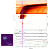 |
Fig. 1. Time profile of a selected event on 10 March 2003. From bottom to top: time profile of the X-ray count rates (corrected from attenuator states) observed with RHESSI in four energy bands (3–6 keV, 6–12 keV, 12–25 keV, and 25–50 keV); time profile of the NRH radio flux at three frequencies (327 MHz, 228 MHz, and 150 MHz) computed on the squared region shown in the insert on the left; and a combination of radio spectrograms in the 1 GHz–20 kHz range obtained with PHOENIX-2 for frequencies above 100 MHz, NDA for frequencies between 10 and 80 MHz, and WIND/WAVES for frequencies below 10 MHz. Insert on the left: position of the type III radio source at the time of the 150 MHz peak. The blue circle represents the position of the optical solar limb and the square shows the region for which the radio flux was computed. |
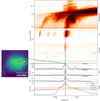 |
Fig. 2. Same as Fig. 1, but for the event selected on 26 August 2011. The HXR count rates are provided by Fermi/GBM in four energy bands: 4–8 keV; 9–14 keV; 15–25 keV; and 25–50 keV. |
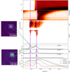 |
Fig. 3. Same as Fig. 2, but for the event selected on 22 April 2013. The radio spectrograph for frequencies above 100 MHz is from ORFEES. Two events were selected and considered in the study during the period plotted. The positions of the type III sources at 150 MHz for the two events are plotted on the left. The white box in the top figure is due to a data gap in the RAD2 instrument. |
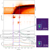 |
Fig. 4. Same as Fig. 3, but for the event selected on 20 October 2013. The HXR data are from RHESSI. Two events were selected and considered in the study during the period plotted. The positions of the type III sources at 150 MHz for the two events are plotted on the right. |
3. Data analysis
For each of the shortlisted events, systematic analyses of their radio and HXR emissions were carried out. For both analyses, we used the standard SolarSoftware(SSW) packages developed for these instruments.
3.1. General description of events
Figures 1–4 show examples of events observed by RHESSI or Fermi in the HXR domain and PHOENIX or ORFEES in the radio domain between 100 MHz and 10 GHz. Figure 1 shows the event that occurred at 10:03 UT on 10 March 2003. A well-defined peak is seen in the HXR energy range (up to energies above 25 keV). We also show the light curves corresponding to the radio flux (see next section) at three frequencies: 150, 228, and 327 MHz. The peak corresponding to the 150 MHz is marked by a straight line. The peak flux at each frequency was computed by subtracting, from the flux at the peak point, the background defined as the mean flux before the event. The HXR spectrum was computed for a 20 s time interval centred around the 150 MHz peak flux. The top panel is the combination of emissions detected by the different radio instruments starting from PHOENIX in the decimetric range, NDA in decametric range, and WIND/WAVES in the kilometric range. The 10 March 2013 event is an example of a simple association between HXR emission above 25 keV and a well-defined type III burst extending from 400 MHz to the IP medium.
Figure 2 depicts the event that occurred on 26 August 2011 at 09:02 UT. The HXR counts were measured using Fermi. The HXR radio association is clearly seen. As in the previous case, the straight line indicates the peak time at 150 MHz. Peaks are coincident in time for HXR and NRH at the three frequencies shown. The few type IIIs seen before the event below 100 MHz and with no HXR counterparts are not included in the study.
Figure 3 shows two type III bursts occurring within a period of a few minutes. Two events with significant HXR counts above 15 keV and well-identified radio emissions at 150 MHz are considered in the present study. Figure 4 similarly shows two events considered in our study occurring on 20 October 2013. Here the type III burst is not detectable at 327 MHz. Such repetitive type III bursts were observed for 16 cases and represent 35 events.
Out of the 205 events selected, 88% of them had their HXR peak co-aligned with the peak of NRH at 150 MHz. This is probably a bias of our selection which ensures that X-ray and radio-emitting electrons result from electrons energised simultaneously for radio and X-ray comparisons. This implies a simple morphology where a well-defined HXR peak is co-temporal with a well-defined type III burst above 100 MHz. For the rest of the events, HXR peaks lie within 10 s of the NRH peak at 150 MHz.
3.2. Peak type III radio fluxes as a function of frequency
Observations from the Nançay Radioheliograph were used to estimate the peak fluxes of type III bursts at four frequencies: 150 MHz, 228 MHz, 327 MHz, and 432 MHz. To achieve that, we used the 10s integrated raw data files containing measured visibilities and produced images of the radio type III sources using the standard CLEAN routine implemented in the standard NRH software. These images provide information on the location of the radio type III sources on the solar disc (see e.g., Figs. 1–4). The radio flux of the type III burst was then computed using the standard NRH software on a region enclosing the burst position as shown in Figs. 1–4. The peak flux was then obtained after subtracting the background defined as the mean of the flux before the burst. The time corresponding to the peak for the 150 MHz channel was defined as the peak time. The choice of 150 MHz was made because the number of events exhibiting emissions at higher frequencies progressively reduces. In our event list, only 86% of selected bursts had emission at 228 MHz, which further reduced to 58% for 327 MHz and only 34% for 432 MHz. This trend is similar to the trend which was found in the previous study by Reid & Vilmer (2017).
Figure 5 (left) represents the distribution of the events as a function of peak fluxes at different frequencies. There is a large spread of the peak fluxes for all the frequencies. Figure 5 (right) shows the evolution of the peak NRH flux as a function of frequency. The peak flux clearly decreases as the frequency increases from 150 to 450 MHz. The spectral index fitted to the median value of the fluxes for each frequency is found to be −2.43. This is in good agreement with the value (−2.21) found in the study by Reid & Vilmer (2017) after removing the mean peak flux around 168 MHz.
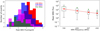 |
Fig. 5. Peak type III radio fluxes. Left: histogram of the NRH peak fluxes at the four selected frequencies. Right: distribution of the NRH peak flux as a function of frequency. The size of the box indicates the interquartile range (IQR) – the range of the 25th percentile to the 75th percentile. The red dots denote the median. A straight-line fit in the log-log space was carried out to the median as shown by the red dashed line. The green triangles are the mean values which are more affected by outliers. |
3.3. Radio starting and stopping frequencies
Starting and stopping frequencies of the type III bursts in our sample were determined using an automated preprocessing pipeline and burst detection algorithm (see Appendix A). Figure 6 (left) shows the distribution of the starting frequencies for all the events of our sample. A large number of events start below 400 MHz. Figure 6 (right) shows the distribution of stopping frequencies of type III bursts. Although it was not a criterion for selection, it is clear that almost all the type III bursts of our sample continue in the IP medium (i.e. below 10 MHz). Only 18 of them have a stopping frequency above 10 MHz. This is most probably due to the fact that the type III bursts selected in our sample are associated with relatively strong X-ray bursts (see the tendency in the previous study by Reid & Vilmer 2017).
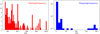 |
Fig. 6. Distribution of starting (left) and stopping (right) frequencies. Given the selection criteria, the starting frequency was purely determined using ORFEES and CALLISTO. A vast majority of the events in our sample extend into interplanetary space. The empty regions of the figure on the right correspond to the frequency bands not covered by observations. |
3.4. HXR spectrum and electron numbers
In this work, our aim is to determine the non-thermal HXR spectrum at the time of the peak flux in the 150 MHz channel. The HXR spectrum observed either by RHESSI or Fermi/GBM was computed on a 20 s time interval centred around this peak (10 s before the peak and 10 s after). Using the OSPEX module in SSW, a combination of a variable isothermal model (red lines in Figs. 7 and 8) and of a non-thermal thick target component (blue lines in Figs. 7 and 8) was fitted to the HXR spectra. The non-thermal component is described by the function thick2 in OSPEX, which directly provides the non-thermal electron spectrum producing HXR emission through thick target radiation. The electron spectrum is represented by a broken power law. Figure 7 shows an example of a spectral fit performed on an event observed by RHESSI (Fig. 1). Since the spectral fit was done only up to 100 keV, only front segments of the detectors were systematically used. Detectors 2 and 7 were also systematically excluded for the whole study because of their degradation mainly after 2006. For each event, RHESSI counts were binned with bin widths of 0.33 keV between 3 and 15 keV and 1 keV between 15 and 100 keV. The figure shows the results of the spectral fit as well as the shape of the non-thermal electron flux deduced from the fit. For the event of 10 March 2003, the electron spectral index below the break δlow is −3.19 while the spectral index above the break δhigh equals −4.52. In that case, the break energy is at 67.2 keV.
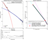 |
Fig. 7. HXR spectral analysis. Left: RHESSI HXR spectrum and fit for the event that occurred on 10 March 2003 (Fig. 1). The figure shows the background-subtracted peak photon spectrum (solid black histogram) overlaid by the total (vth+thick2) spectral fit (light grey line). The red and blue lines show the thermal and the non-thermal components, respectively. Right: non-thermal electron flux deduced from the fit. The integrated electron flux is computed here above the low-energy cutoff 8.37 keV. Bottom: Normalised fit residual as a function of energy. |
Similar spectral fitting is shown in Fig. 8 for an event detected by the Fermi GBM instrument (Fig. 2). Fermi/GBM data consist of 12 NaI detectors which provide full-sky observations. For the present study, we selected data from the most sunward NaI detector (here detector 5). As in the case of RHESSI observations, the spectral fitting was achieved only up to 100 keV. Unlike RHESSI, the energy bins are pre-binned quasilogarithimcally for Fermi. Figure 8 shows the results of the fit for the 22 April 2013 event. The electron spectral index below the break δlow is −4.20 while the spectral index above the break δhigh equals −4.57. In that case, the break energy is at 85.3 keV.
Once the spectral fitting was achieved, the number of non-thermal electrons above variable energy thresholds (low-energy cutoff: 10 keV or 20 keV) at the time of the HXR peak could be directly computed from the fit and this is used in the next section. This estimation was numerically computed as the area under the spectrum using the QUADPACK library in Fortran implemented in Python in the scipy package. The integration was done as a sum of two parts – between 10 or 20 keV and the break energy and between the break energy and 500 keV (since the flux of electrons falls off rapidly above 100 keV). The first term usually dominates the total number of electrons at the time of the HXR peak which is then derived by multiplying, by 20s, the number of electrons/second derived from the fit.
4. Radio type III bursts and HXR electrons
For each event in the present study, the number of HXR-emitting electrons above 10 and 20 keV has been systematically computed at the time of the peak of the associated radio type III burst observed at 150 MHz. Type III radio fluxes observed with the NRH at 228, 327, and 432 MHz were also computed. Scatter plots showing the number of electrons above 20 keV at the time of the type III peak as a function of the peak NRH flux at four frequencies are shown in Fig. 9. The number of events plotted as well as the correlation coefficients are indicated in the figures. Spearman rank-order correlation coefficients are used as they represent a non-parametric measure of the monotonicity of the relationship between two parameters. Due to the spread in the number of electrons and the peak NRH fluxes derived from observations, it is important to estimate the influence of outliers in the estimation of the correlation coefficients. An error analysis was achieved by repeatedly sampling with replacement and estimating the correlation in this sub-sample (bootstrap analysis). For each sampling, 30 data points were chosen and 10 000 such trials were conducted. The median of the distribution of correlation coefficients thus obtained was defined as the true correlation coefficient (indicated in the figure). The standard error was defined as the standard deviation of the distribution of correlation coefficients divided by the square root of the number of trials. Figure 10 shows the results of this bootstrap analysis for peak NRH fluxes versus electron numbers above 10 or 20 keV.
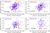 |
Fig. 9. Scatter plot of the type III radio flux at four frequencies versus non-thermal HXR-producing electrons above 20 keV. The number of events for which type III emissions were detected at higher frequencies is indicated and is observed to progressively decrease. The blue points indicate the events that were observed by RHESSI and the red points are the events that were observed by Fermi GBM. Correlation coefficients are 0.38, 0.37, 0.28, and 0.18 for radio frequencies 164 MHz, 228 MHz, 327 MHz, and 432 MHz, respectively. |
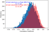 |
Fig. 10. Frequency distribution of correlation coefficient between the type III peak radio flux at 150 MHz and the number of electrons above 10 and 20 keV. The blue distribution corresponds to 10 keV electrons while the red distribution corresponds to 20 keV electrons. We conducted 10 000 trials with 30 data points per sample. |
The correlation coefficients derived from this bootstrap analysis are tabulated in Table 1. It is clear (also see Fig. 9) that the correlation between radio peak fluxes and HXR-producing electrons decreases as the frequency increases. The radio peak fluxes at all frequencies are also more correlated to the number of electrons above 20 keV than to the number above 10 keV, even if the increase in correlation is marginal for 432 MHz.
Correlation coefficients – number of electrons versus peak NRH flux.
A similar analysis was performed between the spectral index of the electron spectra below the break energy (δlow) and the type III peak radio fluxes (it should be noted that for most of the events, the break energy is around 50–80 keV and this is the reason why δhigh is not considered in this analysis). The correlation coefficients are tabulated in Table 2. A weak negative correlation is found for δlow with the peak NRH flux especially at 228 MHz. This suggests that the generation of type III bursts not only depends on the number of electrons above 20 keV, but also on the steepness of the electron spectra in the 20 keV range.
Correlation coefficients – δlow versus peak NRH flux.
Figure 11 finally shows the scatter plot between the starting and stopping frequencies of the type III bursts and the electron number above 10 or 20 keV at the NRH peak, respectively. Some correlation is found between the starting frequency and the electron number. This correlation is stronger for the number of electrons above 20 keV. This suggests that a stronger electron beam will produce type III emission lower in the corona, closer to the acceleration site.
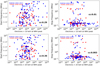 |
Fig. 11. Scatter plot of the electron numbers at the NRH peak above 10 keV and 20 keV versus the starting and stopping frequencies. |
No correlation is found, on the other hand, between the stopping frequency and the electron number. It must however be noted that the bursts associated with the strongest electron numbers (above 1037 for an electron number above 10 keV and above 1036 for an electron number above 20 keV) are systematically observed in the interplanetary medium. This is consistent with the previous results from Reid & Vilmer (2017). More generally, most of the type III bursts in our sample reach the interplanetary medium (only 3% have stopping frequencies above 150 MHz).
5. Discussion and conclusions
In this study, we performed a new statistical analysis on the link between coronal type III bursts and hard X-ray emissions. This is a continuation of the study by Reid & Vilmer (2017) based not only on a new list of events with more stringent selection criteria, but also with a systematic analysis of the HXR spectra allowing for the radio fluxes with the characteristics of HXR-emitting electrons to be compared directly. This has allowed us to use events observed by different HXR instruments and thus to increase the number of events. However, even if the present study is based on thirteen years of observations from 2002 to 2014, the final list of events consists of only 205 cases with a close temporal association between a type III burst at 150 MHz and a significant hard X-ray peak above 12–15 keV (HXR and type III peaks are within 10s). It should be noted that the selection is not done here on the timescale of a flare, but on the timescale of individual bursts in a flare. We summarise the important results of our study below:
-
The type III peak radio flux decreases as a function of frequency in the 450–150 MHz range. There is a large spread in the fluxes at all frequencies as well as in the evolution of the peak flux with frequency, but as a mean the fluxes decrease as ν−2.43. This is consistent with the trend previously observed in the paper by Reid & Vilmer (2017).
-
A rough correlation (correlation coefficient around 0.38) is found between the HXR-producing electron number above 20 keV and the peak type III radio flux at 150 MHz. This correlation decreases with inceasing frequency in the 150–450 MHz range. The correlation is stronger for the electron number above 20 keV than for the electron number above 10 keV.
-
A minor anti-correlation (correlation coefficient around – 0.15) is found essentially at 228 MHz between the absolute value of the spectral index of the HXR-producing electrons in the deka-keV range and the peak radio flux. This anti-correlation decreases at 164 MHz and is null at higher frequencies.
-
A rough correlation (correlation coefficient around 0.36) is found between the HXR-producing electron number above 20 keV and the starting frequency of the type III burst. The correlation is stronger for the electron number above 20 keV than for the electron number above 10 keV.
-
There is no correlation between the stopping frequency of the burst and the HXR-producing electron numbers. Most of the type III bursts of our sample continue in the interplanetary space. This is most probably due to one of our selection criteria since selected type III bursts are associated with relatively strong X-ray bursts (X-ray emission at least to 15 keV) and according to the results of the previous study by Reid & Vilmer (2017), coronal type III bursts associated with significant X-ray emission usually extend to the interplanetary space.
The results of this study reinforce previous results on the connection that exists in simple events between electrons that drive coronal type III emission and X-ray flare emission. In our sample, the close timing between the HXR burst and the peak time of the type III burst as well as the absence of other types of radio emissions favour a situation in which HXR and radio-emitting electrons arise from a common acceleration (injection) site located, for example, in the current sheet that formed above the loop (see e.g., the cartoon from Reid et al. 2014). This choice allowed us to make a detailed association between HXR burst and type III emission, in order to deduce quantitative properties of the non-thermal electrons associated with the generation of type III bursts more precisely.
The present study shows that the HXR-producing electron numbers above 20 keV (resp. above 10 keV) at the peak of the type III bursts range from 1032 to 1038 (resp. a few 1033 to 1039). This can be compared to the total number of electrons in the interplanetary medium estimated to produce a type III burst and which is of the order of 1033 (Lin et al. 1973) as well as to the number of > 10 keV (resp. > 74 keV and > 45 keV) escaping electrons producing interplanetary type III bursts (Krucker et al. 2007; James et al. 2017; Dresing et al. 2021). Generally speaking, the number of electrons producing type III bursts in the interplanetary medium is around 0.1% of the number of electrons necessary to produce X-rays. One of the reasons for this is the rather ineffficient HXR emission process.
The observational results presented in this paper can be interpreted in the context of the results of the many numerical studies of beam-plasma interaction and subsequent production of electromagnetic radiation which have been recently performed (see e.g., Reid et al. 2011; Reid & Kontar 2013, 2018; Li & Cairns 2013; Reid 2020 for a review). These papers deal with the propagation of electron beams injected from a coronal acceleration region upwards in the solar corona, their interaction with Langmuir waves described by a quasi-linear approach, and their subsequent emission of radio emissions (in most cases the fundamental mode of type III bursts). Most of these simulations predict an increase in the type III peak brightness (and then of the peak flux) as a function of decreasing frequency which is observed as a mean in this study as well as in the previous study by Reid & Vilmer (2017). Reid & Kontar (2018) also predict an increase at all frequencies of the peak brightness with an increase in the beam energy density. This could explain why the observations reported here show tendencies of higher peak radio fluxes with an increased number of HXR-emitting electrons (assuming a relationship between upward and downward energetic electrons). The correlation between radio fluxes and electron numbers is better for electrons above 20 keV than for electrons above 10 keV. This tends to show that in the corona, the bump-in-tail distribution (leading to type III radio emission) is rather formed from higher-energy electrons in the 20 keV range. This last conclusion is also supported by the observational result showing a weak anti-correlation between the peak radio fluxes and the electron spectral indices in the 10–30 keV range. Such a weak anti-correlation is consistent with the results of the simulations by Li & Cairns (2013) who found that smaller spectral indices give rise to faster electron beams and produce type III bursts with higher magnitude drift rates but also higher peak values.
The observations also show a decrease with increasing frequencies of the correlation coefficent between electron numbers and peak radio fluxes. In the quasi-linear simulations of electron beam propagation, with an interaction with Langmuir waves and generation of radio emissions, it is found that the ’instability distance’ needed to develop an efficient radio-emitting bump-in-tail distribution) depends on the parameters of the electron beams (spectral index, injection time profile) and on the characteristics of the acceleration site in the corona. In such a context, the increase with decreasing frequency of the correlation between properties of HXR-emitting electrons and radio emissions would be related to an instability distance effect. At high frequencies (435 MHz), the emitting site would be generally too close to the acceleration site and the bump in tail could be not well developed as a mean, while at lower frequencies (150 MHz) the bump-in tail distribution would be formed on a general basis resulting in a stronger relationship between the radio emissions and the number of electrons. The best anti-correlation of the electron spectral index and of the radio peak frequency occurs at 228 MHz. This could be another indication of the mean ‘instability distance’.
Some of the observational results can also be interpreted in the context of alternative interpretations of type III bursts based on electron cyclotron maser theories. In particular, the results of the study by Tang & Wu (2009) show an anti-correlation between the growth rates of the waves (then the peak flux) and the absolute value of the electron spectral index (a harder electron spectrum gives rise to stronger growth rates). This is consistent with the minor anti-correlation found essentially at 228 MHz between the absolute value of the spectral index and the peak radio flux. Moreover, the study by Chen et al. (2021) also shows that the peak growth rate (and thus peak flux) also increases with decreasing emitting frequencies, similarly to the observed increase in peak radio flux with decreasing frequency.
As a final conclusion, the present observational results bring important constraints for further understanding and development of simulations of type III bursts. The characteristics of the HXR-emitting electrons associated with the radio bursts are, however, derived from the emissions clearly detected with instruments such as RHESSI or Fermi/GBM, that is to say in most cases thick-target emissions arising from downward propagating electron beams. Better direct constraints on the properties of type III producing electron beams would result from the direct detection of the X-ray emission produced by upward propagating electron beams. This would require X-ray observations obtained with instruments with higher sensitivities and dynamic ranges such as instruments using focusing optics. As computed by Saint-Hilaire et al. (2009), a total electron number above 10 keV of the order of 1033 could be detected by a HXR direct imager such as FOXSI (Christe et al. 2018). Finally, with Solar Orbiter, the existence on a same platform of X-ray, radio, and particle instruments will also bring many more opportunities in the future to revisit these statistical studies with more events.
Acknowledgments
Tomin James acknowledges the support of the European Commission Horizon 2020 INFRADEV-1-2017 LOFAR4SW project number 777442. Nicole Vilmer acknowledges support from the Centre National d’Études Spatiales (CNES), and from the French programme on Solar-Terrestrial Physics (PNST) of INSU/CNRS for the participation to the RHESSI project. The NRH is funded by the French Ministry of Education and the Région Centre. The Institute of Astronomy, ETH Zürich and FHNW Windisch, Switzerland is acknowledged for funding Phoenix spectrometers. The RHESSI team, the Fermi/GBM team, the WIND/WAVES team and the NRH and ORFEES teams are acknowledged for providing data access and analysis software. The authors acknowledge the Nançay Radio Observatory/Observatoire Radioastronomique de Nançay of the Paris Observatory (USR 704-CNRS, supported by Université d’Orléans, OSUC, and Région Centre in France) for providing access to NDA observations accessible online at http://www.obsnancay.fr. The authors thank the anonymous referee for the useful comments which led to an improved version of the manuscript.
References
- Benz, A. O., Grigis, P. C., Csillaghy, A., & Saint-Hilaire, P. 2005, Sol. Phys., 226, 121 [NASA ADS] [CrossRef] [Google Scholar]
- Benz, A. O., Monstein, C., Beverland, M., Meyer, H., & Stuber, B. 2009, Sol. Phys., 260, 375 [NASA ADS] [CrossRef] [Google Scholar]
- Bougeret, J. L., Kaiser, M. L., Kellogg, P. J., et al. 1995, Space Sci. Rev., 71, 231 [CrossRef] [Google Scholar]
- Chen, L., Wu, D. J., Zhao, G. Q., & Tang, J. F. 2017, J. Geophys. Res. (Space Phys.), 122, 35 [NASA ADS] [CrossRef] [Google Scholar]
- Chen, L., Ma, B., Wu, D., et al. 2021, ApJ, 915, L22 [NASA ADS] [CrossRef] [Google Scholar]
- Christe, S., Shih, A. Y., Krucker, S., et al. 2018, in 2018 Triennial Earth-Sun Summit (TESS), ed. D. Brousseau, 404.144 [Google Scholar]
- Dresing, N., Warmuth, A., Effenberger, F., et al. 2021, A&A, 654, A92 [NASA ADS] [CrossRef] [EDP Sciences] [Google Scholar]
- Fox, N. J., Velli, M. C., Bale, S. D., et al. 2016, Space Sci. Rev., 204, 7 [Google Scholar]
- Hamilton, R. J., Petrosian, V., & Benz, A. O. 1990, ApJ, 358, 644 [NASA ADS] [CrossRef] [Google Scholar]
- Hamini, A., Auxepaules, G., Birée, L., et al. 2021, J. Space Weather Space Clim., 11, 57 [NASA ADS] [CrossRef] [EDP Sciences] [Google Scholar]
- James, T., Subramanian, P., & Kontar, E. P. 2017, MNRAS, 471, 89 [Google Scholar]
- Kane, S. R. 1972, Sol. Phys., 27, 174 [NASA ADS] [CrossRef] [Google Scholar]
- Kane, S. R. 1981, ApJ, 247, 1113 [NASA ADS] [CrossRef] [Google Scholar]
- Kerdraon, A., & Delouis, J. M. 1997, in The Nançay Radioheliograph, ed. G. Trottet, 483, 192 [Google Scholar]
- Klein, K.-L. 2021, Front. Astron. Space Sci., 7, 105 [NASA ADS] [Google Scholar]
- Krucker, S., Kontar, E. P., Christe, S., & Lin, R. P. 2007, ApJ, 663, L109 [CrossRef] [Google Scholar]
- Lecacheux, A. 2000, Geophys. Monogr. Ser., 119, 321 [NASA ADS] [Google Scholar]
- Li, B., & Cairns, I. H. 2013, J. Geophys. Res. (Space Phys.), 118, 4748 [NASA ADS] [CrossRef] [Google Scholar]
- Li, B., Cairns, I. H., & Robinson, P. A. 2008, J. Geophys. Res. (Space Phys.), 113, A06105 [NASA ADS] [Google Scholar]
- Li, B., Cairns, I. H., & Robinson, P. A. 2009, J. Geophys. Res. (Space Phys.), 114, A02104 [NASA ADS] [Google Scholar]
- Lin, R. P., Evans, L. G., & Fainberg, J. 1973, App. Lett., 14, 191 [Google Scholar]
- Lin, R. P., Dennis, B. R., Hurford, G. J., et al. 2002, Sol. Phys., 210, 3 [Google Scholar]
- Meegan, C., Lichti, G., Bhat, P. N., et al. 2009, ApJ, 702, 791 [Google Scholar]
- Melrose, D. B. 1980, Space Sci. Rev., 26, 3 [NASA ADS] [CrossRef] [Google Scholar]
- Messmer, P., Benz, A. O., & Monstein, C. 1999, Sol. Phys., 187, 335 [NASA ADS] [CrossRef] [Google Scholar]
- Müller, D., St. Cyr, O. C., Zouganelis, I., et al. 2020, A&A, 642, A1 [Google Scholar]
- Pick, M., & Vilmer, N. 2008, A&ARv, 16, 1 [NASA ADS] [CrossRef] [Google Scholar]
- Ratcliffe, H., Kontar, E. P., & Reid, H. A. S. 2014, A&A, 572, A111 [NASA ADS] [CrossRef] [EDP Sciences] [Google Scholar]
- Reid, H. A. S. 2020, Front. Astron. Space Sci., 7, 56 [NASA ADS] [CrossRef] [Google Scholar]
- Reid, H. A. S., & Kontar, E. P. 2013, Sol. Phys., 285, 217 [NASA ADS] [CrossRef] [Google Scholar]
- Reid, H. A. S., & Kontar, E. P. 2018, ApJ, 867, 158 [NASA ADS] [CrossRef] [Google Scholar]
- Reid, H. A. S., & Vilmer, N. 2017, A&A, 597, A77 [NASA ADS] [CrossRef] [EDP Sciences] [Google Scholar]
- Reid, H. A. S., Vilmer, N., & Kontar, E. P. 2011, A&A, 529, A66 [NASA ADS] [CrossRef] [EDP Sciences] [Google Scholar]
- Reid, H. A. S., Vilmer, N., & Kontar, E. P. 2014, A&A, 567, A85 [NASA ADS] [CrossRef] [EDP Sciences] [Google Scholar]
- Saint-Hilaire, P., Krucker, S., Christe, S., & Lin, R. P. 2009, ApJ, 696, 941 [NASA ADS] [CrossRef] [Google Scholar]
- Tang, J. F., & Wu, D. J. 2009, A&A, 493, 623 [NASA ADS] [CrossRef] [EDP Sciences] [Google Scholar]
- Vilmer, N. 2012, Philos. Trans. R. Soc. London Ser. A, 370, 3241 [NASA ADS] [Google Scholar]
- Wang, W., Wang, L., Krucker, S., et al. 2021, ApJ, 913, 89 [NASA ADS] [CrossRef] [Google Scholar]
- Wu, C. S., Wang, C. B., Yoon, P. H., Zheng, H. N., & Wang, S. 2002, ApJ, 575, 1094 [NASA ADS] [CrossRef] [Google Scholar]
- Wu, D. J., Chen, L., Zhao, G. Q., & Tang, J. F. 2014, A&A, 566, A138 [NASA ADS] [CrossRef] [EDP Sciences] [Google Scholar]
Appendix A: An algorithm to extract the radio burst from background
To reliably estimate the starting and stopping frequencies, we developed a novel method, using computer vision techniques, to extract the burst out of the background. This is essential because the emissions are detected using different instruments with a different base background. Because the final frequency spectrum was constructed out of data from three different radio instruments, the inherent sampling rates available were also different. This poses a problem for computer vision algorithms since they work in the pixel space and not in the frequency space. To overcome this problem, we equalised the sampling rate of all the instruments to 1 second, which was the native time cadence for NDA. This meant for CALLISTO and WAVES that we had to upsample the data. For upsampling, we used the linear interpolation of the nearest values of a pixel. However, for ORFEE we had to downsample to get to 1 second time cadence. For this purpose, we used a Gaussian averaging with an anti-aliasing filter to avoid image artefacts. The re-sampled spectrograms were combined in the time axis to form a single spectrogram of the chosen time cadence.
To determine the background, we had to define the noise level. This was done in two ways – both manually and using an adaptive threshold algorithm. In the first step, we defined global threshold limits by removing the outliers. This was done by removing bad frequency channels and then calculating the median iteratively such that the brightest pixel was at least 10% more in magnitude than the average median value. This way we ensured a robust signal-to-noise ratio, even after removing the outliers. We defined an area of interest around the peak time of the 150 MHz flux determined from the NRH. The remaining signal above the noise level threshold after this stage is predominantly that from the radio burst with various small band RFI signals intermixed, especially along the communication bands. Using an adaptive threshold algorithm, we generated contours on this image. The adaptive threshold was defined as those pixels that had a gradient increase of more than 50% in comparison to neighbouring pixels. These pixels were then grouped and linked together to form bigger groups that defined the outline of the burst. Since radio bursts have a predominantly elongated shape profile along the frequency axis, we defined an elongated rectangle as a block kernel. This block kernel was then convoluted with the contours locally. This ensured that local frequency disturbances, which are usually elongated along a time axis, got averaged out. Since only the pixels grouped as belonging to the burst were sampled, we ended up isolating the burst from the background. The starting and stopping frequencies were estimated from the pixelised reconstruction of the burst.
We show an example in Fig A.1. We were interested in extracting the second burst which occurred at 10:26 UT (Fig 3). The spectrogram is plotted on a linear scale. There is increased noise in the NDA because of the common normalisation employed instead of normalising individually for each instrument. There are some data gaps in the rad 1 and rad 2 instrument. After running it through the algorithm with a convolution kernel of the size shown in the lower left of the second panel, we were able to extract the major contours of the burst. The starting frequency of the burst was found to be 374 MHz while the stopping frequency was found to be 0.24 MHz.
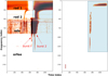 |
Fig. A.1. Burst extraction algorithm in action for an event on 22 April 2013. On the left-hand side, the primary data are plotted. We note that there are two bursts in the present figure but that the extraction is shown here for the second burst (blue bounding box). The figure on the right shows the pixelised representation of the second type III burst, once the algorithm had been applied. The starting and stopping frequencies were found to be 374 MHz and 0.24 MHz, respectively. |
All Tables
All Figures
|
Fig. 1. Time profile of a selected event on 10 March 2003. From bottom to top: time profile of the X-ray count rates (corrected from attenuator states) observed with RHESSI in four energy bands (3–6 keV, 6–12 keV, 12–25 keV, and 25–50 keV); time profile of the NRH radio flux at three frequencies (327 MHz, 228 MHz, and 150 MHz) computed on the squared region shown in the insert on the left; and a combination of radio spectrograms in the 1 GHz–20 kHz range obtained with PHOENIX-2 for frequencies above 100 MHz, NDA for frequencies between 10 and 80 MHz, and WIND/WAVES for frequencies below 10 MHz. Insert on the left: position of the type III radio source at the time of the 150 MHz peak. The blue circle represents the position of the optical solar limb and the square shows the region for which the radio flux was computed. |
| In the text | |
|
Fig. 2. Same as Fig. 1, but for the event selected on 26 August 2011. The HXR count rates are provided by Fermi/GBM in four energy bands: 4–8 keV; 9–14 keV; 15–25 keV; and 25–50 keV. |
| In the text | |
|
Fig. 3. Same as Fig. 2, but for the event selected on 22 April 2013. The radio spectrograph for frequencies above 100 MHz is from ORFEES. Two events were selected and considered in the study during the period plotted. The positions of the type III sources at 150 MHz for the two events are plotted on the left. The white box in the top figure is due to a data gap in the RAD2 instrument. |
| In the text | |
|
Fig. 4. Same as Fig. 3, but for the event selected on 20 October 2013. The HXR data are from RHESSI. Two events were selected and considered in the study during the period plotted. The positions of the type III sources at 150 MHz for the two events are plotted on the right. |
| In the text | |
|
Fig. 5. Peak type III radio fluxes. Left: histogram of the NRH peak fluxes at the four selected frequencies. Right: distribution of the NRH peak flux as a function of frequency. The size of the box indicates the interquartile range (IQR) – the range of the 25th percentile to the 75th percentile. The red dots denote the median. A straight-line fit in the log-log space was carried out to the median as shown by the red dashed line. The green triangles are the mean values which are more affected by outliers. |
| In the text | |
|
Fig. 6. Distribution of starting (left) and stopping (right) frequencies. Given the selection criteria, the starting frequency was purely determined using ORFEES and CALLISTO. A vast majority of the events in our sample extend into interplanetary space. The empty regions of the figure on the right correspond to the frequency bands not covered by observations. |
| In the text | |
|
Fig. 7. HXR spectral analysis. Left: RHESSI HXR spectrum and fit for the event that occurred on 10 March 2003 (Fig. 1). The figure shows the background-subtracted peak photon spectrum (solid black histogram) overlaid by the total (vth+thick2) spectral fit (light grey line). The red and blue lines show the thermal and the non-thermal components, respectively. Right: non-thermal electron flux deduced from the fit. The integrated electron flux is computed here above the low-energy cutoff 8.37 keV. Bottom: Normalised fit residual as a function of energy. |
| In the text | |
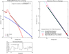 |
Fig. 8. Same as Fig. 7, but for the 22 April 2013 event observed by Fermi/GBM. |
| In the text | |
|
Fig. 9. Scatter plot of the type III radio flux at four frequencies versus non-thermal HXR-producing electrons above 20 keV. The number of events for which type III emissions were detected at higher frequencies is indicated and is observed to progressively decrease. The blue points indicate the events that were observed by RHESSI and the red points are the events that were observed by Fermi GBM. Correlation coefficients are 0.38, 0.37, 0.28, and 0.18 for radio frequencies 164 MHz, 228 MHz, 327 MHz, and 432 MHz, respectively. |
| In the text | |
|
Fig. 10. Frequency distribution of correlation coefficient between the type III peak radio flux at 150 MHz and the number of electrons above 10 and 20 keV. The blue distribution corresponds to 10 keV electrons while the red distribution corresponds to 20 keV electrons. We conducted 10 000 trials with 30 data points per sample. |
| In the text | |
|
Fig. 11. Scatter plot of the electron numbers at the NRH peak above 10 keV and 20 keV versus the starting and stopping frequencies. |
| In the text | |
|
Fig. A.1. Burst extraction algorithm in action for an event on 22 April 2013. On the left-hand side, the primary data are plotted. We note that there are two bursts in the present figure but that the extraction is shown here for the second burst (blue bounding box). The figure on the right shows the pixelised representation of the second type III burst, once the algorithm had been applied. The starting and stopping frequencies were found to be 374 MHz and 0.24 MHz, respectively. |
| In the text | |
Current usage metrics show cumulative count of Article Views (full-text article views including HTML views, PDF and ePub downloads, according to the available data) and Abstracts Views on Vision4Press platform.
Data correspond to usage on the plateform after 2015. The current usage metrics is available 48-96 hours after online publication and is updated daily on week days.
Initial download of the metrics may take a while.