| Issue |
A&A
Volume 673, May 2023
|
|
|---|---|---|
| Article Number | A137 | |
| Number of page(s) | 20 | |
| Section | The Sun and the Heliosphere | |
| DOI | https://doi.org/10.1051/0004-6361/202245412 | |
| Published online | 18 May 2023 | |
Comparison of chromospheric diagnostics in a 3D model atmosphere
Hα linewidth and millimetre continua
1
Rosseland Centre for Solar Physics, University of Oslo, Postboks 1029 Blindern, 0315 Oslo, Norway
2
Institute of Theoretical Astrophysics, University of Oslo, Postboks 1029 Blindern, 0315 Oslo, Norway
e-mail: This email address is being protected from spambots. You need JavaScript enabled to view it.
Received:
8
November
2022
Accepted:
24
March
2023
Abstract
Context. The Hα line, one of the most studied chromospheric diagnostics, is a tracer of magnetic field structures, while the intensity of its line core provides an estimate of the mass density. The interpretation of Hα observations is complicated by deviations from local thermodynamic equilibrium (LTE) or instantaneous statistical equilibrium conditions. Meanwhile, millimetre (mm) continuum radiation is formed in LTE, and therefore the brightness temperatures from Atacama Large Millimetre-submillimetre Array (ALMA) observations provide a complementary view of the activity and the thermal structure of stellar atmospheres. These two diagnostics together can provide insights into the physical properties of stellar atmospheres, such as their temperature stratification, magnetic structures, and mass density distribution.
Aims. In this paper, we present a comparative study between synthetic continuum brightness temperature maps at mm wavelengths (0.3 mm to 8.5 mm) and the width of the Hα 6565 Å line.
Methods. We used the 3D radiative-transfer codes Multi3D and Advanced Radiative Transfer (ART) to calculate synthetic spectra for the Hα line and the mm continua, respectively, from an enhanced network atmosphere model with non-equilibrium hydrogen ionisation generated with the state-of-the-art 3D radiation magnetohydrodynamics (rMHD) code Bifrost. We use a Gaussian point spread function (PSF) to simulate the effect of ALMA’s limited spatial resolution and calculate the Hα versus mm continuum correlations and slopes of scatter plots for the original and degraded resolution of the whole box, quiet sun, and enhanced network patches separately.
Results. The Hα linewidth and mm brightness temperatures are highly correlated and the correlation is highest at a wavelength of 0.8 mm, that is, in ALMA Band 7. The correlation systematically increases with decreasing resolution. On the other hand, the slopes decrease with increasing wavelength. The degradation of resolution does not have a significant impact on the calculated slopes.
Conclusions. With decreasing spatial resolution, the standard deviations of the observables, Hα linewidth, and brightness temperatures decrease and the correlations between them increase, but the slopes do not change significantly. These relations may therefore prove useful in calibrating the mm continuum maps observed with ALMA.
Key words: radiative transfer / Sun: chromosphere / Sun: radio radiation / line: profiles / methods: numerical / radio continuum: stars
© The Authors 2023
 Open Access article, published by EDP Sciences, under the terms of the Creative Commons Attribution License (https://creativecommons.org/licenses/by/4.0), which permits unrestricted use, distribution, and reproduction in any medium, provided the original work is properly cited.
This article is published in open access under the Subscribe to Open model. This email address is being protected from spambots. You need JavaScript enabled to view it. to support open access publication.
1. Introduction
One of the most commonly used chromospheric diagnostics is the Hα line, that is, the transition between atomic levels 3 and 2 in the hydrogen atom (Cram & Mullan 1985). Because of its high opacity in the line core, the Hα line core forms in the low plasma beta regime, where there is more dominant magnetic pressure than the plasma pressure, which results in magnetic fields being the main structuring agent in the upper chromosphere (Leenaarts et al. 2012). For this reason, the Hα line is a very good diagnostic for the magnetic structures in the chromosphere. The chromospheric mass density can be traced with the Hα line core intensity (Leenaarts et al. 2012). The low atomic mass of hydrogen results in high-temperature sensitivity of the Hα line width through significant thermal Doppler broadening (Cauzzi et al. 2009). Even though the Hα line is a useful diagnostic of stellar chromospheres –because it forms in non-local thermodynamic equilibrium (NLTE)–, it is not particularly suitable for determination of the chromospheric temperature stratification (Pasquini & Pallavicini 1991).
Based on radiative-transfer calculations for a solar atmospheric radiation–magnetohydrodynamics (rMHD) simulation (Carlsson et al. 2016), Leenaarts et al. (2012) show that the Hα line width is correlated with the temperature of the plasma, while the line core intensity is a diagnostic of the mass density in the chromosphere. These relations come from the fact that the Hα line is a strongly scattering line such that the source function is non-locally determined by the mean intensity. A high local temperature means that the atomic absorption profile becomes wide (because of the low atomic mass, the width of the profile is dominated by thermal broadening), and we also get a wide intensity profile because the source function is rather insensitive to the local conditions. A high mass density in the chromosphere leads to line-core formation at a larger height where the source function is lower, and therefore lower line-core intensity.
It is well established that the continuum radiation at millimetre (mm) wavelengths is formed at chromospheric heights (see e.g. Wedemeyer et al. 2016, and references therein). The continuum radiation at mm wavelengths (here 0.3–8.5 mm) originates from free-free emission in the chromosphere, and the two main opacity sources are H and H− free-free absorption (Dulk 1985). These processes result in a LTE source function as they are coupled to the local property of the plasma: the electron temperature. We can therefore use the Rayleigh-Jeans law and interpret the emergent intensity (the observed brightness temperature (Tb)) in the mm wavelength domain as local electron temperature (Loukitcheva et al. 2015). For this reason, the mm continuum is a very convenient diagnostic for understanding the temperature stratification in solar and stellar atmospheres (Wedemeyer-Böhm et al. 2007; Wedemeyer et al. 2020).
The Hα line opacity is proportional to the hydrogen n = 2 level population; the Hα optical depth scales with the n = 2 column density (Leenaarts et al. 2007). The availability of free electrons is dependent on the n = 2 population of hydrogen in the upper atmosphere (Molnar et al. 2019). The formation of the Hα and mm continuum is influenced by the plasma temperature, the H(n = 2) level populations, and electron populations.
Traditional Hα activity indicators, such as linewidth, full width at half maximum (FWHM), or integrated fluxes depend on several wavelengths across the line profile (Hanuschik 1989; Gizis et al. 2002; Marsden et al. 2014; Molnar et al. 2019). The Hα line core is formed higher in the atmosphere than the wings, and therefore while calculating these activity indicators from observations, we inherently look at a large volume of plasma in the chromosphere (Vitas et al. 2009), which makes determining the thermal stratification difficult. In this regard, the mm continuum has an additional advantage as a complementary diagnostic, namely that –to a first approximation– the radiation at a given mm wavelength originates from approximately the same height range with the average formation height range increasing as a function of wavelength. While this assumption is probably valid on average, we note that the exact formation height ranges might show variations because of the surface corrugation, which is investigated here (see e.g. Eklund et al. 2021; Wedemeyer et al. 2022; Hofmann et al. 2022, and references therein). On the other hand, the formation height of the Hα line is in the range of 0.5 Mm to 3 Mm above the photosphere, which is a large range (Leenaarts et al. 2012).
The Atacama Millimetre/submillimetre Array (ALMA; Wootten & Thompson 2009) provides observations with a high spatial and temporal resolution for the mm continuum. The Hα linewidth and mm continua both depend on the temperature and the electron density of the volume of plasma where they are formed. In the present work, we focus on using these two as complementary diagnostics, similar to the case study on co-observational data for ALMA Band 3 and IBIS in Molnar et al. (2019). Here, we compare the mm continuum and Hα linewidth synthesised from a 3D realistic Bifrost model atmosphere to understand how these can be used as complementary diagnostics for the chromosphere. Our model and spectral synthesis are described in Sect. 2. In Sect. 3, we present a quantitative comparison of the two diagnostics, which is further qualitatively discussed in Sect. 4. Finally, we present our conclusions in Sect. 5.
2. Methods
We used a snapshot of a numerical 3D simulation of the solar atmosphere (see Sect. 2.1) as input for radiative-transfer codes to compute the Hα line intensity (see Sect. 2.2) and the continuum intensity at mm wavelengths (see Sect. 2.5). We then degraded the resulting maps for different wavelengths to a spatial resolution typically achieved with ALMA as described in Sect. 2.6, before determining the Hα line width and comparing it to the mm brightness temperatures.
2.1. Three-dimensional model atmosphere
Bifrost is a 3D radiation magnetohydrodynamics (rMHD) simulation code that includes physics relevant to chromospheric conditions (Gudiksen et al. 2011). The model used for this study is taken from a continuation of the enhanced network simulation en024048 at 17 min after the publicly released snapshots from Carlsson et al. (2016). The computational box of this model extends 24 Mm × 24 Mm horizontally, and vertically from 2.4 Mm below the visible surface to 14.4 Mm above it, thereby encompassing the upper part of the convection zone, the photosphere, chromosphere, transition region, and corona. The computational box consists of 504 × 504 × 496 grid points with a horizontal resolution of 48 km, which corresponds to an angular size of approximately 0.066 arcsec. The grid is non-equidistant in the vertical direction, varying from 19 km in the photosphere and chromosphere up to a height of 5 Mm and then increasing to 100 km at the top boundary. Both the top and bottom boundaries are transparent, whereas lateral boundary conditions are periodic. At the bottom boundary, the magnetic field is passively advected with no extra field fed into the computational domain. For further details, see Carlsson et al. (2016, and references therein).
The temperature and absolute magnetic field showing the loops of the enhanced network with the quiet region at typical chromospheric heights are shown in Fig. 1. As seen in Figs. 11 and 12 in Carlsson et al. (2016), the simulation has different regions. The en024048 simulation features an enhanced network (EN) patch with loops in the middle of the computational domain as seen in Fig. 2 in Loukitcheva et al. (2015) or (see the black square in Figs. 3 and 4), whereas the outer parts are more representative of magnetically less active, quiet Sun (QS) conditions. In the absolute magnetic field slice through 1.74 Mm (Fig. 1b), the footpoints of the magnetic loops are seen. The gas temperatures at those heights are comparatively lower at locations with higher magnetic strengths, and the loops show significantly higher temperatures in the range of 2 to 3 MK from the footpoint to the apex of the loop.
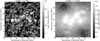 |
Fig. 1. Horizontal cross-section of temperature (left) and the absolute magnetic field ( |
2.2. Hα spectral line synthesis
Multi3D (Leenaarts et al. 2009) employs the accelerated lambda iteration method developed by Rybicki & Hummer (1992) with the extension to treat effects of partial frequency redistribution using the angle averaged approximation by Uitenbroek (2001). We used a five-level plus continuum hydrogen model atom. Microturbulence is not introduced, as Leenaarts et al. (2012) show that the synthesised spectra are similar to observational spectra even without using microturbulence. Further details of how the Hα spectra are synthesised in 3D using Multi3D can be found in Leenaarts et al. (2012).
2.3. Hα observations of α Cen A
In this study, H α observations of the solar-like star α Cen A are used for comparison. The data were acquired from Porto de Mello et al. (2008) and Lyra & Porto de Mello (2005). The Hα observations were collected at Observatório do Pico dos Dias (OPD), which is operated by the Laboratório Nacional de Astrofísica (LNA), CNPq, Brazil on the ESPCOUDE 1.60m telescope. The data were wavelength-calibrated, Doppler-corrected, and flux-normalised to unity by Porto de Mello et al. (2008).
2.4. Definition of linewidth
As this study is based on forward modelling, we use the definition of linewidth put forward by Leenaarts et al. (2012). However, we note that different definitions of the Hα linewidth are used in the literature. The definition of core width given by Leenaarts et al. (2012) and the definitions used by Cauzzi et al. (2009) and Molnar et al. (2019) are compared to the definition of FWHM for the linewidth in Fig. 2
 |
Fig. 2. Comparison of the linewidth as defined by Molnar et al. (2019; upper panel), by Leenaarts et al. (2012; middle panel) and as defined as the FWHM (lower panel). The red, black and green lines show normalised spectra for the VAL C model, Bifrost QS and the observed spectrum for α Cen A (Porto de Mello et al. 2008), respectively. The solid blue lines in the top panel mark ± 1 Å, while the dotted lines show the considered maxima and the dashed lines show the calculated linewidths in all three cases. |
The Leenaarts et al. (2012) Hα line-core width calculated for the Bifrost model is the full width at one-tenth maximum, which is the separation between the line wings at I = Imin + 0.1(Imax − Imin). The representative wavelengths for the red and blue line wing that span the core width are calculated by first identifying the two spectral sampling points which are closest to one-tenth of the intensity between the pseudo continuum and the line core and then using linear interpolation.
Molnar et al. (2019) follow the definition by Cauzzi et al. (2009) for their observational study, and these authors define linewidth as the separation of the line profile wings at half of the line depth, where the maxima are defined at ± 1 Å from the line core (referred to as the Molnar et al. (2019) definition of linewidth hereafter). The line-core intensity calculated for the Bifrost model used in this study reveals the structure of the EN loops. The variation in the activity in the model atmosphere among QS and EN regions is also visible from the variation of the Hα line core intensity. It is to be noted that throughout the paper, the wavelengths mentioned are vacuum wavelengths.
The resulting line core width according to the Leenaarts et al. (2012) definition is shown in Fig. 3a. Please note that the plotted value ranges for these maps have been limited to the 99th to 1st percentile for better visibility, and in particular to highlight the imprints of the loop structures in contrast to the less active surroundings.
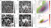 |
Fig. 3. Comparisons of the Hα line core width (a,d) and ALMA at 3.0 mm brightness temperature maps (b,e) at original (top row) and degraded (bottom row) resolution. The black and red boxes on these maps denote the chosen EN and QS regions, respectively. The last column is a correlation contour plot between the Hα linewidth and ALMA brightness temperature at 3.0 mm, with contours with linear fits (dashed lines) and means (circles) of the three cases: the whole simulation box in red, the QS box in green, and the EN region box in blue. The red and green star data points are for the FAL C and VAL C 1D semi-empirical models and the black circle with error bars is an observational data point for the G2V type star α Cen A with a linewidth of 0.62 Å. |
2.5. Synthesis of mm continuum brightness temperatures
The intensity of the continuum radiation at mm wavelengths for the 3D input model (see Sect. 2.1) is calculated with the Advanced Radiative Transfer (ART) code by de la Cruz Rodríguez et al. (2021). The output intensities Iλ are then converted to brightness temperatures Tb using the Rayleigh-Jeans approximation:
 (1)
(1)
where, λ, kB, and c are the wavelength and Boltzmann constant and the speed of light, respectively. In total, maps for 34 wavelengths are computed, covering the range that in principle can be observed with ALMA. This includes both currently available receiver bands and bands that might be offered for solar observations in the future. The resulting maps for the wavelengths of 3.0 mm and 0.8 mm are presented in Figs. 3 and 4, respectively, while further maps for selected wavelengths are shown in Appendix A (Figs. A.1–A.8).
2.6. Image degradation
In principle, the synthesised beam for interferometric observations with ALMA, that is, the effective point spread function (PSF), depends on several factors, such as the angle of the Sun in the sky with respect to the array baselines and the configuration of the antennas. The resulting beam would be typically elliptical, while the Fourier space of the source (here the Sun) would only be sampled sparsely (see e.g. Högbom 1974; Boone 2013). For this theoretical study, circular Gaussians are used as PSFs as a first approximation, as this simplified approach is sufficient to demonstrate the effect of spatial resolution. The more detailed modelling of the ALMA beam would depend on the exact array configuration, receiver band (some of which are not yet used for solar observations), and details of the imaging process, which would go beyond the scope of this study (Wedemeyer et al. 2022).
As mentioned above, the exact shape and width of the synthetic beam varies even for observations in the same receiver band. For instance, the data sets found on the Solar ALMA Archive (SALSA, Henriques et al. 2022) have widths of around 2″, which includes the beam with a width of 1.92″ × 2.30″ for the data set 2016.1.01129.S. That data set was also used by Mohan et al. (2021), although their choice of imaging parameters results in a beam width of only 1.75″ × 1.91″. However, based on a comparison with Hα observations, these latter authors instead chose a PSF with a width of 1.95″ × 2.03″. For simplicity in this study, the width of the beam (i.e. the PSF) is set to 2″ at a wavelength of λ = 3.0 mm and is then linearly scaled as a function of the observing wavelength λ. The considered wavelength range includes the receiver bands that are already available for solar observations with ALMA (bands 3, 5 and 6, i.e. 2.59–3.57, 1.42–1.90 and 1.09–1.42 mm), but in addition also bands 1, 2, 4, and 7–10, thereby covering the whole range that might be offered in the future from 0.3 mm to 8.5 mm. The same wavelength-dependent Gaussian kernels are used for degrading the mm brightness temperature maps and the Hα intensity maps. Please note that all three considered snapshots (with 5 min solar time between snapshots) are synthesised and then degraded with the different beams. In addition, corresponding time-averaged ALMA maps are calculated so that they can be compared to the observational data used by Molnar et al. (2019).
2.7. Semi-empirical models
For comparison, the 1D semi-empirical reference models Vernazza-Avrett-Loeser C (VAL C; Vernazza et al. 1981) and Fontella-Avrett-Loeser C (FAL C; Fontenla et al. 1993) are used, which are both representative of quiet Sun conditions. Corresponding Hα line profiles and mm continuum intensities for these 1D semi-empirical atmosphere models are calculated with the radiative code RH (Uitenbroek 2001; Pereira & Uitenbroek 2015).
3. Results
3.1. Dependence on spatial resolution
Figure 3 shows a comparison between the EN and QS regions for the original and the degraded resolution corresponding to the assumed ALMA resolution at a wavelength of 3 mm. The calculated Hα line core width for the whole box (panel a) is very similar to the results in Fig. 9a in Leenaarts et al. (2012). The Hα line core width from the simulation (Fig. 9a in Leenaarts et al. 2012) appears to be formed at a lower height in the chromosphere than that suggested by observations (Fig. 16b in Leenaarts et al. 2012). As the employed wavelength points are very close to the line core, one should expect to see chromospheric features in the line-core width map. However, in contrast, the continuum intensity for 3 mm at the original resolution as shown in Fig. 3b differs notably from the line-core width shown in Fig. 3a.
The maps appear more similar at reduced resolution after convolution with a circular Gaussian kernel corresponding to the spatial resolution at the wavelength of 3 mm (see panels (d) and (e)). The black and red boxes on these maps denote the chosen EN and QS regions for further comparison. The EN region is chosen to be centred at the EN as seen in the degraded resolution, and the QS region is placed at the bottom right corner of the simulation box. Both boxes are of the same size, of namely 9.5 Mm × 9.5 Mm (200 pixels × 200 pixels).
Panels (c) and (f) of Fig. 3 show the scatter contour plots for the three sets of pixels: the whole simulation box, the QS box (red square in panels a,b,d,e), and the EN box (black square in panels a,b,d,e). The distribution for the whole simulation box is shown in red contours with the colour bar for the number of pixels falling into the individual bins. The QS and EN distributions are represented by green and blue contours, respectively. The distributions at the original resolution show substantially more spread than the distributions at degraded resolution because of the associated loss of variations on small spatial scales. This effect is already clear from a visual comparison of the Hα linewidth maps in panels (a) and (d) and likewise for the mm brightness temperature maps in panels (b) and (e), respectively. The red, green, and blue points in panels (c) and (f) represent the average values for the whole box, QS and EN, respectively. The impact of applying the ALMA beam can be seen from the spatial power spectral density plots in Fig. 5. As seen in the plots for 3.0 mm and 0.8 mm, the power spectral density (PSD) falls drastically for small spatial scales that are not resolved with the respective PSF (beam). Another notable observation is that both definitions of linewidth show similar values of power at larger scales. At smaller scales, the mm PSD is close to the PSD of the line-core-width definition, implying better correlations (see Table 1). Also, the observational 3 mm data show a very similar trend in PSD to the mm spatially degraded data, as expected.
Brightness temperatures in kK, correlation coefficients, and slopes for the three pixel sets (whole box, QS, and EN) each for two resolutions (original and degraded) for the single snapshot and time-averaged dataset, with both the definitions used for calculating the linewidth.
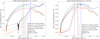 |
Fig. 5. Normalised power spectral density kPk plots for time-averaged datasets of mm brightness temperatures with both definitions of linewidth at 3.0 mm and 0.8 mm. The solid lines represent the original-resolution data and the dashed lines show the spatially degraded data, green for the Leenaarts et al. (2012) linewidth, red for the Molnar et al. (2019) definition of linewidth, and blue for the corresponding mm wavelength. The vertical lines represent the dominant spatial scales (in arcsec) for the original-resolution data with the (Leenaarts et al. 2012) definition of linewidth and the Molnar et al. (2019) definition of linewidth. The black dashed line represents the PSF corresponding to the mm wavelength, showing the resolution limit for the degraded dataset. In the left panel, the spatial power spectral density for the Band 3 ALMA observations (ADS/NRAO.ALMA#2016.1.01129.S) as used by Molnar et al. (2019) and shown in Fig. 11 are plotted as the black solid line. The power spectral density was calculated for all time steps in the time range considered by Molnar et al. (2019) and then averaged in time. |
In addition, the Hα linewidth and the Tb at the mm wavelengths for the VAL C and FAL C semi-empirical model atmospheres are plotted for comparison. The VAL C model has consistently lower brightness temperature than the FAL C model, as seen in Fig. 6. When plotted on the linewidth-versus-temperature planes, these QS models lie in between the EN and QS distributions, demonstrating the agreement between the data from our study and the semi-empirical models. Applying the beam changes the mean Tb value for the QS and EN pixel sets as shown in Table 1. The mean EN Tb decrease and mean QS Tb increase leave the mean Tb of the whole box unchanged. This change in the mean and standard deviation of the brightness temperatures is further shown in Fig. 6 and discussed in Sect. 4.1. The Tb at 3 mm for the VAL C and FAL C models are calculated as 7009 K and 7624 K, respectively, which are similar to the corresponding average brightness temperature of 6968 K across the whole horizontal extent of the 3D model employed here (see Table 1). The value for FAL C agrees with the calculations reported by Loukitcheva et al. (2004). The differences are further discussed in comparison to observations in Sect. 4.2 It should also be noted that the average QS Tb = 6621 K found for the 3D model is lower than the reference value of 7300 K suggested by White et al. (2017) for Band 3 (λ = 3.0 mm) at the centre of the solar disk. Please refer to Sect. 4.2 for further discussion.
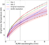 |
Fig. 6. Comparison of the mean brightness temperatures for mm wavelengths at the resolution of the original simulations (in black) and the resolution of the observations from the ALMA observatory (in red). In both these cases, the whole simulation box (solid lines), the QS box (dotted lines), and the EN box (dashed lines) are taken separately. The pink and blue shaded regions show a region of one standard deviation around the mean for the original resolution and the degraded resolution case, respectively. The green and blue dashed lines show brightness temperature trends for FAL C and VAL C models, respectively. The black dashed vertical lines mark 0.8 mm and 3 mm. |
The wavelength of 0.8 mm is of particular interest for this study, too, as will be discussed in Sects. 3.2 and 4.2. The results for λ = 0.8 mm are presented in Fig. 4, which corresponds to the above-discussed Fig. 3 for λ = 3.0 mm. While the Hα line core width map at the original resolution (panel a) is the same in both figures, the mm brightness temperature maps (panel (b)) and the degraded maps (panels (d) and (e)) differ. The Hα line core width map (Fig. 4a) and the mm continuum map at 0.8 mm (Fig. 4b) are already very similar at the original resolution and even more so at the lower resolution, as shown in Fig. 4d-e. The PSF at 0.8 mm is smaller in width compared to the 3.0 mm PSF by a factor of 0.8/3.0, which can be seen from a visual comparison of Fig. 3e and Fig. 4e. The 3.0 mm maps appear more blurred, mainly as a result of the wider PSF. The same effect can be seen for the Hα line width maps, which were derived from the Hα line-intensity maps after these were all degraded accordingly for each wavelength point.
The slopes in the EN and QS cases are very similar to each other and are also similar to the slopes for the whole box as seen in Table 1. In contrast to Fig. 3c and f, the scatter plots in Fig. 4c and f show that the slopes for the QS and EN distributions (0.052 and 0.045) are very similar to the values for the maps at degraded resolution. On the other hand, for 3 mm, the values are 0.03 and 0.029, which show a higher departure from each other. The mean Tb values for the QS region and the whole box are relatively close, as seen in Table 1, as the atmosphere is mainly QS. The VAL C and FAL C data points are closer to the mean Tb for the EN region, possibly because of the factors discussed above. Treating the synthetic mm and the Hα linewidth map with the generated PSFs for corresponding wavelengths (see Appendix A for representative plots similar to Figs. 3 and 4 for ALMA bands), the scatter and the linear fits were plotted and the slopes and the correlation coefficients were calculated. The trends in correlations and slopes for all considered wavelengths are presented in Sect. 3.2 and shown in Figs. 7 and 8, respectively.
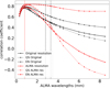 |
Fig. 7. Comparison of the calculated Pearson correlation coefficients with two different resolutions. Black vertical lines show the ALMA band 3 range and black horizontal lines show the Molnar et. al. correlation coefficient = 0.84. and the red vertical line shows the maximum correlation in the original resolution case, which is at 0.8 mm. |
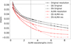 |
Fig. 8. Comparison of the calculated slopes for the scatter plots, legend same as Fig. 6. The black lines show the Molnar et. al. slope = 0.0612 at 3 mm. |
3.2. Correlations and slopes
The correlation of the Hα linewidth maps and the mm brightness temperature maps and the dependence of this correlation on mm wavelength and therefore spatial resolution are quantified through the Pearson correlation coefficient between the Hα linewidth maps and mm brightness temperature maps and linear fits to the distributions, as shown for example in Figs. 3 and 4. The slopes, as well as the intercept of the linear fits, are calculated by linear regression for the whole box, and the EN and QS regions, separately.
The resulting correlation coefficients as a function of wavelength are shown in Fig. 7 at original resolution (black lines) and after degradation with the synthetic ALMA PSFs (red lines) corresponding to the wavelength. It should be noted that the mm brightness temperature maps exhibit differences as a function of wavelength which are due to the different formation height ranges at a given wavelength. Although the formation heights can vary notably across the model, they nonetheless increase on average with increasing wavelength. Consequently, the mm brightness temperature maps at original resolution show a maximum correlation with the Hα linewidth maps at a given wavelength as can be seen most clearly from the peak for the QS correlation (black dotted line) for wavelengths in the range from 0.5 mm to 1.8 mm. Peaks are also present for the whole box and the EN region with a decrease towards shorter and longer wavelengths in all cases.
Reducing the spatial resolution has a notable impact on the correlation coefficients (see Fig. 7), resulting in generally higher values as compared to the correlation at the original resolution. The QS region correlations are lower than for the whole box in both cases and the EN region correlations are slightly higher in the degraded resolution case and for most wavelengths for the original resolution. While the correlation for the degraded resolution maps also exhibits peaks, there is a systematic increase in the correlation between the degraded resolution maps as a function of wavelength for longer wavelengths. This effect can be attributed primarily to the spatial resolution, that is, the width of the PSF, which increases with wavelength. Consequently, the structure below a corresponding (small) spatial scale is blurred, which affects the resulting correlation coefficient. With increasing wavelength, more and more of this atmospheric fine structure is blurred, as already discussed in Sect. 3.1 and seen from a comparison of Figs. 3 and 4 (see Table 1 for the correlation coefficients for 3.0 mm and 0.8 mm). However, at the longest wavelengths, even structure on relatively large spatial scales is lost. Consequently, the data ranges for these very blurred maps become very narrow, which then results in a high correlation coefficient. The impact of a lower spatial resolution on the data ranges is also visible in Fig. 3c,f and 4c,f: The shown distributions become notably narrower as a function of spatial resolution for the whole box, QS region, and EN region, being broadest at the original resolution and narrowest when degraded with the 3.0 mm PSF. Most importantly, the highest correlation for the degraded maps with a value of 0.844 is found for the EN region at 1.1 mm, whereas the QS region has a maximum of 0.839 at 1.0 mm. The correlation for the whole box peaks with 0.799 at a wavelength of 1.0 mm as well. These results suggest that (i) the highest correlation between the Hα line core width and mm continuum brightness temperature maps is found for wavelengths at 1.0 mm, which corresponds to ALMA Band 7, and that (ii) the correlation between observed Hα line core width maps and simultaneously obtained ALMA Band 7 brightness temperature maps is expected to be higher than what was found by Molnar et al. (2019) for Band 3 observations (at 3.0 mm); see Sect. 4.2 for further discussion.
The blue contours in Fig. 4c and f, which represent the EN region, show higher Hα line core widths and mm brightness temperatures. On the other hand, the green contours, which represent the QS regions, show lower intensities in mm and lower Hα linewidths in both resolutions; these differences are more distinct in the degraded resolution case. As the smaller network–internetwork features get blurred, the higher (lower) intensities in the QS (EN) region get blurred with neighbouring lower (higher) intensities and hence the green (blue) contours shift downwards (upwards). The slopes of the fitted lines for the three distributions change with resolution. The slope decreases for the EN case but increases for the QS case with the degraded resolution, as can be seen in Fig. 8 for all the cases in the dataset.
The slopes show a general decreasing trend with wavelength. As the wavelength increases, the radiation originates from a slightly higher layer of the atmosphere, which is on average slightly hotter. As seen in Fig. 6, the temperatures at different wavelengths are dependent on the formation heights, in addition to the resolution. This is evident from the decreasing slopes shown in Fig. 8. For the degraded resolution case, the difference in the slope for QS and EN regions is more than the original resolution case. In particular, for the EN case, as seen in Figs. 3 and 4, in the degraded resolution case (panels d and e), the brightness temperatures decrease, decreasing slopes significantly. For the QS case, on the other hand, the slopes remain comparable, or approximately the same in both resolutions. This is explained by the blurring effect due to the application of the ALMA PSFs, but in the QS region, the features are more equally distributed. The slopes therefore do not significantly change with the resolution in the mm range of interest (Bands 3-6). The line widths derived from the time-averaged Hα intensity maps following the definition by Molnar et al. (2019) produce very similar trends and also indicate that the best match occurs at wavelengths corresponding to ALMA Band 7. Please refer to Sects. 3.3 and 4.2 for further discussion.
3.3. Dependence on temporal resolution
Figures 9 and 10 show the original and ALMA resolution maps for the dataset averaged over 10 min. The comparison of features in Figs. 9a,b and 3a,b with those in Figs. 10a,b and 4a,b shows that the time averaging causes the features to smooth out, as expected. The QS, EN, and whole box contours show less spread in the time-averaged case than in the single snapshot case, as observed in Figs. 9c,f and 3c,f and Figs. 10c,f and 4c,f, respectively. When calculating the Hα line core width from the time-averaged maps and comparing it to the time-averaged mm brightness temperature maps, the correlation between the Hα line core width maps and the mm brightness temperature maps at original resolution decreases, whereas the correlation increases significantly for the corresponding maps at reduced (i.e. ALMA) resolution. The correlation is highest for the EN case and the lowest for the QS case at both resolutions. This can be attributed to the differences in the small-scale features in the QS region, which get averaged over time and therefore do not match in the two data sets at degraded resolution. Similarly, the slopes for the QS region are also lower than for the whole box, whereas the slopes for the EN region are higher than for the whole box. The slopes do not show very drastic changes from the single snapshot case, but they are monotonically decreasing for all pixel sets.
4. Discussion
The Hα line core widths correlate best with the mm continuum brightness temperatures at a wavelength of 0.8 mm. The Pearson correlation coefficients for the degraded maps are determined as 0.778 for the whole box, 0.808 for the QS region, and 0.834 for the EN region (see Table 1). These results imply that, despite the similarities of the Hα linewidth with the observational ALMA Band 3 data found by Molnar et al. (2019), a closer match with Band 7 is to be expected. The immediate next step would therefore be to compare observational ALMA Band 7 data with co-observed Hα data but, to the best of our knowledge, no such data are currently available for the study presented here.
4.1. Effect of spatial resolution
One of the aims of this study is to use high-resolution synthetic data at mm wavelengths to investigate how they can complement other diagnostics, such as Hα, for determining the properties of small-scale features in the solar atmosphere. Even though the resolution of ALMA observational data is outstanding compared to previous observations at mm wavelengths, the resolution is very low compared to what is typically achieved at optical wavelengths (see e.g. White et al. 2006; Wedemeyer et al. 2016, and references therein).
The comparison between maps at the original resolution and maps at the ALMA resolution using Gaussian kernels as simplified PSFs for the respective wavelengths (see Figs. 3 and 4) shows that there are two effects in action: the change in the formation layer for the mm data, and the decreasing resolution due to the increasing wavelength. These two effects cannot be disentangled in observational data, but with a simulation like the one employed here the physical and instrumental effects can be separated. In Fig. 6, the effect of the change in formation height for the continuum radiation at mm wavelengths and the change in resolution for the given wavelength are demonstrated. Although the average brightness temperature of the whole simulation box remains the same when degrading the resolution at a given wavelength, the width of the brightness temperature distribution (as represented by the shaded areas of one standard deviation around the mean values in the figure) reduces with degrading resolution. The increase in correlations and a general decrease in slopes with the degradation of the resolution can be attributed to this phenomenon.
To understand this impact of the spatial resolution more quantitatively, the values of the correlations for all six cases for λ = 0.8 mm and λ = 3.0 mm are listed in Table 1. The correlations significantly increase with the degradation of the resolution, as observed in Fig. 7. On the other hand, as seen in Fig. 8 and Table 1, the slopes do not change significantly. Hence, it can be safely speculated that the Hα linewidth and mm brightness temperatures are correlated and follow the linear fit fairly well.
Figure 16 presents the formation heights for the continuum at wavelengths of 3.2 mm, 1.8 mm, and 0.8 mm, along with the vertical temperature slice through the model atmosphere. Two more formation height profiles are plotted for the linewidth definition by Molnar et al. (2019; cf. Cauzzi et al. 2009) and for the line core width as defined by Leenaarts et al. (2012). In both cases, the plotted line is the average formation height of the wavelength points in the blue and red line wing that result from the calculation of the linewidth. It is observed that the Leenaarts et al. (2012) definition agrees better with the 0.8 mm formation height range. The Molnar et al. (2019) linewidth is rather a diagnostic of the lower atmosphere.
4.2. Comparison with observations
To compare these results with the observational study by Molnar et al. (2019), we used the same definition of the linewidth, which follows the approach by Cauzzi et al. (2009, see Sect. 2.4). The corresponding Hα and mm maps at the original and degraded resolution with the scatter contour plots are shown in Figs. 12 and 13. In Figs. 14c,f and 15c,f, the black dashed lines show the respective correlation and slope calculated by Molnar et al. (2019) for the observational data obtained with ALMA in Band 3 (3 mm) on 23 April 2017 (see their Fig. 3). We produced a brightness temperature map similar to the one shown in Fig. 3 by Molnar et al. (2019) by time-averaging the corresponding data that is publicly available on the Solar ALMA Science Archive (SALSA, Henriques et al. 2022; see Fig. 11). The differences between the data from Molnar et al. (2019) and the data taken from SALSA are due to the difference in the applied imaging, including the choice of CLEAN parameters and the combination of the interferometric and total power (TP) data, as Molnar et al. (2019) follow the standard approach while the SALSA data are produced with the Solar ALMA Pipeline (Wedemeyer et al. 2020). Please refer to White et al. (2017) and Shimojo et al. (2017) for a detailed discussion of the uncertainties of the interferometric and TP data, which both affect the resulting absolute brightness temperatures. A cutout from the central part of the observed field of view with the same extent as the synthetic observations presented here (i.e. 24 Mm × 24 Mm) is shown in Fig. 11b to allow for a direct comparison. Within the 1st and 99th percentiles, the brightness temperature range is observed to be between 5 kK and 11 kK both in the observational data and the simulated data (see Fig. 3e), in particular given the aforementioned uncertainties in absolute brightness temperatures derived from ALMA observations. This qualitative agreement with observations was already demonstrated for a different snapshot of the same Bifrost simulation by Loukitcheva et al. (2015); see also Loukitcheva et al. (2004). As mentioned in Sect. 3.1, the average brightness temperature at 3.0 mm for the whole computational box of the 3D model is only ∼100 K higher than the corresponding value for the VAL C model and only 520 K lower than the FAL C value. These therefore all agree with the reference value of 7300 K derived by White et al. (2017) from ALMA observations within the aforementioned uncertainties.
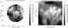 |
Fig. 11. Time-averaged ALMA Band 3 brightness temperature for the same measurement set as used by Molnar et al. (2019), i.e. ADS/NRAO.ALMA#2016.1.01129.S from 23 April 2017. The data were averaged over the period from 17:31 to 17:41 UTC. (a) The whole FOV. (b) The central 24 Mm × 24 Mm part, also indicated by the red box in panel (a) for comparison with the simulated data. |
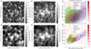 |
Fig. 12. Same as Fig. 9, for the Molnar et al. (2019) definition of linewidth. The black dashed line denotes the linear fit by Molnar et al. (2019). |
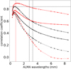 |
Fig. 14. Same as Fig. 7, but for the time-averaged data set, for the Molnar et al. (2019) definition of linewidth. The legend is the same as for Fig. 7 |
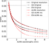 |
Fig. 15. Same as Fig. 8, but for the time-averaged data set, for the Molnar et al. (2019) definition of linewidth. |
The resolution of the observed ALMA data shown in Fig. 11 appears to be lower than for the degraded maps presented in Fig. 4e, which can be attributed to several factors. Firstly, as detailed in Sect. 2.6, the synthetic brightness temperatures maps are degraded to ALMA’s angular resolution by convolution with ideal PSFs, each of which is constructed as a circular Gaussian with a width appropriate for the respective wavelength. This simplified approach corresponds in principle to a telescope with a filled aperture of the size of the longest baseline. However, in reality, ALMA consists of a limited number of antennas in a given configuration, which results in a sparse sampling of the spatial Fourier space of the observed source. The resulting PSF (or rather referred to as synthesised beam) of the interferometric array is typically elongated and tilted. Properly accounting for these detailed instrumental effects, the additional degradation due to Earth’s atmosphere and the necessary imaging of the ALMA data (see e.g. Henriques et al. 2022) requires a much more detailed and computationally more expensive modelling approach (Wedemeyer et al. 2022), which goes beyond the scope of the study presented here. However, overall it is safe to assume that the employed degradation of the synthetic brightness temperature maps is still too optimistic. The same is true for the synthetic Hα data for which further instrumental effects and the influence of the Earth’s atmosphere are not accounted for. The statement that the employed instrumental degradation for ALMA is still too optimistic is confirmed by the power spectral density shown for the ALMA Band 3 in Fig. 5. The curve for the observational data starts to drop at a slightly larger spatial scale as compared to the simulated data and also shows a noise component at smaller spatial scales that is not included in the simulations here.
Secondly, the ALMA image shown in Fig. 11 represents the time-average over an observational period of 10 min, which is produced in the same way as described by Molnar et al. (2019). Also, the Hα observations obtained with IBIS by Molnar et al. (2019) were time-averaged for a comparison with the aforementioned ALMA data. A period of 10 min is substantial given the dynamic timescales on which the chromospheric fine structure evolves, and the time-averaging further blurs the resulting images. This effect can be seen by comparing, for example, Figs. 3e and 12e, but it is also apparent in Fig. 3 by Molnar et al. (2019), which compares snapshots to time-averaged images. In Table 1, the correlation coefficients and the slopes for both cases are listed.
Thirdly, limited spectral sampling points for the IBIS observations (Cavallini 2006) and also the time it takes to scan through the spectral line profile would contribute to uncertainties. For our simulated data, we used more than three times more spectral sampling points for the Hα line, namely 101, as compared to the 29 points for the IBIS data used by Molnar et al. (2019).
As a result of the limited resolution discussed above, emission from different heights gets mixed within the respective synthesised ALMA beam. It is particularly important to be aware of this effect in view of the highly dynamic and intermittent nature of the solar chromosphere, which can result in substantial changes in formation height across small (possibly unresolved) spatial distances. In addition, it should be noted that the region observed by Molnar et al. (2019) comprises a mix of plage, network, and magnetically quiet regions, whereas the simulated data contain only EN and QS regions and can therefore only be compared within the respective limitations.
As a result of these effects, differences in the density plot for Hα linewidth versus ALMA brightness temperature for the simulated data in Fig. 12f and the corresponding density plot for observed data in Molnar et al. (2019, see their Fig. 4) are expected. However, it should be noted that, despite these effects, the distributions in observed and simulated data are very similar. The simulated QS distribution coincides with the high-density scatter distribution at low observed brightness temperatures and low Hα line widths in the plot shown by Molnar et al. (2019). The blue EN contour, which has a slightly lower slope than the slopes for the QS part and the slope for the whole box in the simulated data, has its counterpart in the scatter plot for the observed data. The calculated slopes for the whole box at the degraded resolution are slightly different, which can be attributed to the aforementioned differences between the observations and the simulations reported here. For the observed data, Molnar et al. (2019) report the slope to be 0.0612, as compared to 0.015 for the whole box at degraded spatial and temporal resolution for the simulated data (see Table 1 for details).
As shown in Sect. 3.2, changing the spatial resolution affects the correlations between Hα linewidth and mm brightness temperatures. The correlation for the data observed at 3 mm reported by Molnar et al. (2019) is 0.84, which is close to the correlation of 0.61 found here for the simulated data at degraded spatial and temporal resolution. The correlation is 0.5 for the data at the original resolution. The difference in the correlation coefficients is because the spatial arrangement of the individual pixels relative to each other does not matter when calculating them. Consequently, the correlation coefficient increases with decreasing spatial resolution, because the resulting image degradation gradually removes the largest variations on the smallest scales in both the ALMA and the Hα maps. For both data sets, lowering the spatial resolution results in narrower intensity distributions towards the mean value. The height at which the core is formed is higher and the linewidth is lower for the quiet region, and the formation height is lower and linewidth is higher for the EN region (Leenaarts et al. 2012).
4.3. Effect of temporal resolution
When time-averaging the spatially degraded Hα and mm brightness temperature maps, the resulting correlation coefficients change with respect to the results based on single snapshots. As summarised in Table 1, for the line core width as defined by Leenaarts et al. (2012), the correlation coefficients for all three pixel sets become lower when time-averaging both at original and reduced resolution, except for a small increase for the correlation with the 3 mm data across the whole box at reduced resolution (cf. Fig. 14). The same behaviour is found when using the linewidth definition by Molnar et al. (2019), except perhaps for a small increase of the EN correlations both at original and reduced spatial resolution.
In general, temporal averaging results in blurring of the maps and lower correlation coefficients. However, for the EN region, time-averaging can tend to highlight persistent features, resulting in a slightly higher correlation coefficient. In contrast, for the QS region, the more uniformly distributed and short-lived features get averaged over time and space and lose the similarities. Similarly, the values of slopes for original and degraded resolutions are very close for individual wavelengths (see Fig. 15). In conclusion, time averaging causes a decrease in the correlation in the QS case and a small increase in the EN case for the Molnar definition, while the slopes decrease marginally. This effect becomes slightly more notable for the maps at reduced spatial resolution as compared to the maps at original resolution. We conclude that the exact values and behaviour of correlation coefficients as shown here may depend critically on the spatial and temporal resolution of the employed data.
4.4. Comparison of linewidth definitions
As seen in Fig. 2, the value and the atmospheric layer connected to the linewidth change significantly based on the definition used. In the case of the Molnar et al. (2019) definition, as described in Sect. 2.4, the continuum and therefore the line depth are derived from the ±1 Å region around the line core. On the other hand, for both the Leenaarts et al. (2012) definition and the FWHM, the continuum is defined based on the true continuum intensity. The wavelength grid points used for the calculation of the line core width –which are close to the line core– are formed significantly higher in the atmosphere than they are when taking the Molnar et al. (2019) approach, as illustrated in Fig. 16. The radiation at the wavelength points in the line wings as used for the FWHM definition are accordingly formed lower in the atmosphere, even lower than for the Molnar et al. (2019) definition. In Fig. 17, the line widths for all three definitions are compared, implying the above-discussed differences in connected atmospheric heights, which are highest for the line-core width definition by Leenaarts et al. (2012). The FWHM linewidth map much resembles a granulation pattern as formed in the low photosphere.
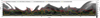 |
Fig. 16. Simulated logarithmic gas temperature (grey-scale) in a vertical slice of 3D rMHD Bifrost simulations. The solid lines represent the heights at which the optical depth is unity at a wavelength of 3.2 mm (red), and 0.8 mm (green), which correspond to ALMA bands 3, 5 and 7, respectively. The orange, white and yellow lines show the average heights at which the red and blue sides of the Hα line width according to the Leenaarts et al. (2012), Molnar et al. (2019) and FWHM definitions of linewidth are formed. |
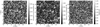 |
Fig. 17. Maps of linewidths for original resolution case for the single snapshot: Left: Leenaarts et al. (2012) definition, middle: Molnar et al. (2019) definition and right: FWHM. |
The distribution of line core widths as seen in Fig. 18a is in the range of line core widths calculated by Leenaarts et al. (2012). Using the Molnar et al. (2019) definition instead produces larger linewidths (see Fig. 18b), which nonetheless remain smaller than the observationally determined values reported by Molnar et al. (2019). The simulated linewidths according to the Molnar et al. (2019) definition cover a range of 0.75 to 1.0. Å, whereas the values derived from observations by Molnar et al. (2019) are in the range of 0.9 to 1.3 Å, which is also in line with the observed linewidth for α Cen A (see Sect. 4.5). The reason behind this discrepancy could be that the Hα opacity used in the simulations that include the radiative transfer calculations is lower than that for the real Sun (Leenaarts et al. 2012). Similarly, as seen in Fig. 16, the formation heights of the radiation at the wavelength positions entering the line-core width calculation with the Leenaarts et al. (2012) definition are closer to the formation heights of the mm continua than to the corresponding heights for the Molnar et al. (2019) definition. The conclusion that the Leenaarts et al. (2012) definition produces a better match of the Hα line (core) width with the mm continua is also implied by a closer match in terms of spatial power spectral density as compared to the Molnar et al. (2019) definition (see Fig. 5). This seems to be true at both the original and reduced resolutions.
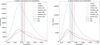 |
Fig. 18. Left: Distribution of Hα line core widths (following the definition by Leenaarts et al. 2012) for the whole time series. Right: Corresponding line widths according to the definition by Molnar et al. (2019). The whole box, QS and EN regions are separately plotted in blue, black and red, and mean and median values for the three sets of pixels are indicated with a dot-dashed and dashed lines in the respective colours. Please note the difference in ranges for linewidths axes in the two plots. |
4.5. Implications for solar-like stars
The correlation between Hα linewidth and mm brightness temperatures described in Sect. 3.2 can be transferred to the study of Sun-like stars. It should be noted that the study presented here is based on simulated EN and QS regions, while the corresponding trends for a whole active region could not be investigated because of the lack of an equivalent consistent simulation. Any comparison with unresolved observations of other solar-like stars therefore needs to account for the potential contributions of active regions via corresponding filling factors.
A direct application to stellar observations is to estimate the stellar activity level, in particular for Sun-like stars as for instance used in the studies by Liseau et al. (2016) and Mohan et al. (2021, 2022). The position in the Hα linewidth–mm brightness temperature plane as derived from adequate observations then provides constraints on the properties of the observed stellar atmosphere. This approach is illustrated by comparing the data points for the semi-empirical 1D models FAL C and VAL C to the averages for the whole box, EN, and QS data points on the Hα linewidth–mm brightness temperature plane in Figs. 3 (c and f) and 4 (c and f). For the disk-integrated signal, the centre-to-limb variation for the Hα line and ALMA full disk data should be taken into account (see e.g. Alissandrakis et al. 2022a,b; Otsu et al. 2022; Nindos et al. 2018, and references therein). As the Hα core forms in the chromosphere and the wings in the photosphere, the limb effects would be varying (brightening or darkening depending on the wavelength) when going from the core to the wing. In a recent study based on SST observations, Pietrow et al. (2022) concluded that chromospheric lines might exhibit a blueshift towards the limb due to the chromospheric canopies, but the resulting effect on the equivalent width or linewidths is non-trivial. Further, the authors show that the line core widths would decrease when going from the centre to the limbs. Further systematic studies need to be conducted in order to understand the limb effects on the correlations between the two diagnostics and the implications for disk-integrated stellar observations.
The brightness temperature values at the wavelengths of 0.8 mm and 3 mm for α Cen A, which are obtained from ALMA observations (see Mohan et al. 2021, and references therein), are in line with the values derived from ALMA observations of the Sun and also with those based on the simulations presented in this study. In contrast, the Hα line profile for α Cen A (see Fig. 2), with a line core width of ∼0.6 Å, is significantly broader than the simulated data based on the Bifrost simulation and also for the FAL C and VAL C models, which causes the respective data point to be placed away from the linear fit for the solar simulation shown in Figs. 3 (c and f) and 4 (c and f); see the black circle with error bars in these figures. The α Cen A datapoint is out of the bounds of the plane in Figs. 12 (c and f) and 13 (c and f) as the calculated Molnar et al. (2019) linewidth is 1.1 Å. The comparatively broad Hα line profile for α Cen A is likely due to differences in atmospheric structure and the activity level of this star as compared to the Sun; although an in-depth study would be needed to in order to draw any detailed conclusions. We also note that the solar observations are spatially resolved and cover only a small region on the Sun, whereas the α Cen A data are intrinsically integrated across the whole (spatially unresolved) stellar disk.
5. Conclusions
We look at the synthetic Hα linewidth and the brightness temperatures corresponding to the mm wavelengths generated from a close-to-realistic 3D Bifrost model. Degrading the spatial resolution of these synthetic observations to ALMA resolution results in decreased standard deviations of the synthetic observables: Hα line width and mm brightness temperatures, and increased correlations between them. With increasing wavelength, the beam size increases and the small structures get blurred out, resulting in a further increased correlation between the two diagnostics. But this degradation in terms of spatial resolution does not have any significant effect on the mean slopes for the linear fits on the Hα linewidth versus mm brightness temperature distributions. This implies that the instrumental resolution of ALMA is sufficient to capture the similarities between the two diagnostics.
The solar results in comparison with the observations of α Cen A strongly imply that the Hα linewidth and mm continuum brightness temperatures can be considered equivalent indicators; as shown in Fig. 16, they form close to each other and the thermal stratification of a star can be constrained using the correlations and slopes found in this study in the absence of mm data, simply using the Hα data, and vice versa. As discussed in Wedemeyer et al. (2016, see also references therein), using multi-wavelength observations along with mm observations can provide better insights into the thermal structure of stellar atmospheres.
The Hα linewidth depends on the temperature in the line-forming region, which is observed using mm continua (Leenaarts et al. 2012). The brightness temperatures can be directly calculated from the mm continuum intensity maps, which correlate with the Hα linewidth very well. The best match, that is, in terms of the highest correlation, is found for a wavelength of 0.8 mm, which corresponds to ALMA Band 7. Simultaneous Hα–ALMA Band 7 observations have therefore the potential advantage of better constraining the imaging process, resulting in more reliable temperature measurements for the solar chromosphere. Published simulations of the solar chromosphere (Carlsson et al. 2016) show overly narrow MgII h & k lines compared with IRIS observations (Carlsson et al. 2019), indicating that the models have too little mass at upper chromospheric temperatures. Newer models in higher resolution, including ambipolar diffusion and non-equilibrium ionisation (e.g., Martínez-Sykora et al. 2023), flux emergence (Hansteen et al. 2023), or run with the MURaM code with chromospheric extensions (Przybylski et al. 2022), show significantly broader magnesium lines. It will be important to check the reported ALMA-Hα relationships with these new models. As the correlation between the two diagnostics is high even in the case of lower resolution, this study may prove useful in mitigating the challenging task of calibrating mm continuum solar data obtained from ALMA.
Acknowledgments
We thank the referee for very valuable comments and suggestions, which improved considerably the quality of this paper. This work is supported by the Research Council of Norway through the EMISSA project (project number 286853), the Centres of Excellence scheme, project number 262622 (“Rosseland Centre for Solar Physics”) and through grants of computing time from the Programme for Supercomputing. This paper makes use of the following ALMA data: ADS/NRAO.ALMA#2016.1.01129.S. ALMA is a partnership of ESO (representing its member states), NSF (USA) and NINS (Japan), together with NRC (Canada), MOST and ASIAA (Taiwan), and KASI (Republic of Korea), in cooperation with the Republic of Chile. The Joint ALMA Observatory is operated by ESO, AUI/NRAO and NAOJ. The authors thank Porto de Mello et al. (2008) for their prompt correspondence regarding the Hα observational data of α Cen A. This research utilised the Python libraries matplotlib (Hunter 2007), seaborn (Waskom 2021) and the NumPy computational environment (Oliphant 2006). The authors would like to thank Thore Espedal Moe, Mats Ola Sand, Atul Mohan, Juan Camilo Guevara Gomez, Vasco Henriquez, Shahin Jafarzadeh for their support.
References
- Alissandrakis, C. E., Bastian, T. S., & Brajša, R. 2022a, Front. Astron. Space Sci., 9, 981320 [NASA ADS] [CrossRef] [Google Scholar]
- Alissandrakis, C. E., Bastian, T. S., & Nindos, A. 2022b, A&A, 661, L4 [NASA ADS] [CrossRef] [EDP Sciences] [Google Scholar]
- Boone, F. 2013, Exp. Astron., 36, 77 [NASA ADS] [CrossRef] [Google Scholar]
- Carlsson, M., Hansteen, V. H., Gudiksen, B. V., Leenaarts, J., & De Pontieu, B. 2016, A&A, 585, A4 [NASA ADS] [CrossRef] [EDP Sciences] [Google Scholar]
- Carlsson, M., De Pontieu, B., & Hansteen, V. H. 2019, ARA&A, 57, 189 [Google Scholar]
- Cauzzi, G., Reardon, K., Rutten, R. J., Tritscheenaarter, A., & Uitenbroek, H. 2009, A&A, 503, 577 [NASA ADS] [CrossRef] [EDP Sciences] [Google Scholar]
- Cavallini, F. 2006, Sol. Phys., 236, 415 [NASA ADS] [CrossRef] [Google Scholar]
- Cram, L. E., & Mullan, D. J. 1985, ApJ, 294, 626 [NASA ADS] [CrossRef] [Google Scholar]
- de la Cruz Rodríguez, J., Szydlarski, M., & Wedemeyer, S. 2021, https://zenodo.org/record/4604825 [Google Scholar]
- Dulk, G. A. 1985, ARA&A, 23, 169 [Google Scholar]
- Eklund, H., Wedemeyer, S., Szydlarski, M., & Jafarzadeh, S. 2021, A&A, 656, A68 [NASA ADS] [CrossRef] [EDP Sciences] [Google Scholar]
- Fontenla, J. M., Avrett, E. H., & Loeser, R. 1993, ApJ, 406, 319 [Google Scholar]
- Gizis, J. E., Reid, I. N., & Hawley, S. L. 2002, AJ, 123, 3356 [Google Scholar]
- Gudiksen, B. V., Carlsson, M., Hansteen, V. H., et al. 2011, A&A, 531, A154 [NASA ADS] [CrossRef] [EDP Sciences] [Google Scholar]
- Hansteen, V. H., Martinez-Sykora, J., Carlsson, M., et al. 2023, ApJ, 944, 131 [NASA ADS] [CrossRef] [Google Scholar]
- Hanuschik, R. W. 1989, Ap&SS, 161, 61 [NASA ADS] [CrossRef] [Google Scholar]
- Henriques, V. M. J., Jafarzadeh, S., Guevara Gómez, J. C., et al. 2022, A&A, 659, A31 [NASA ADS] [CrossRef] [EDP Sciences] [Google Scholar]
- Hofmann, R. A., Reardon, K. P., Milic, I., et al. 2022, ApJ, 933, 244 [NASA ADS] [CrossRef] [Google Scholar]
- Högbom, J. A. 1974, A&AS, 15, 417 [Google Scholar]
- Hunter, J. D. 2007, Comput. Sci. Eng., 9, 90 [NASA ADS] [CrossRef] [Google Scholar]
- Leenaarts, J., & Carlsson, M. 2009, ASP Conf. Ser., 415, 87 [Google Scholar]
- Leenaarts, J., Carlsson, M., Hansteen, V., & Rutten, R. J. 2007, A&A, 473, 625 [NASA ADS] [CrossRef] [EDP Sciences] [Google Scholar]
- Leenaarts, J., Carlsson, M., & Rouppe van der Voort, L. 2012, ApJ, 749, 136 [NASA ADS] [CrossRef] [Google Scholar]
- Liseau, R., De la Luz, V., O’Gorman, E., et al. 2016, A&A, 594, A109 [NASA ADS] [CrossRef] [EDP Sciences] [Google Scholar]
- Loukitcheva, M., Solanki, S. K., Carlsson, M., & Stein, R. F. 2004, A&A, 419, 747 [NASA ADS] [CrossRef] [EDP Sciences] [Google Scholar]
- Loukitcheva, M., Solanki, S. K., Carlsson, M., & White, S. M. 2015, A&A, 575, A15 [NASA ADS] [CrossRef] [EDP Sciences] [Google Scholar]
- Lyra, W., & Porto de Mello, G. F. 2005, A&A, 431, 329 [NASA ADS] [CrossRef] [EDP Sciences] [Google Scholar]
- Marsden, S. C., Petit, P., Jeffers, S. V., et al. 2014, MNRAS, 444, 3517 [Google Scholar]
- Martínez-Sykora, J., de la Cruz Rodríguez, J., Gošić, M., et al. 2023, ApJ, 943, L14 [CrossRef] [Google Scholar]
- Mohan, A., Wedemeyer, S., Pandit, S., Saberi, M., & Hauschildt, P. H. 2021, A&A, 655, A113 [NASA ADS] [CrossRef] [EDP Sciences] [Google Scholar]
- Mohan, A., Wedemeyer, S., Hauschildt, P. H., Pandit, S., & Saberi, M. 2022, A&A, 664, L9 [NASA ADS] [CrossRef] [EDP Sciences] [Google Scholar]
- Molnar, M. E., Reardon, K. P., Chai, Y., et al. 2019, ApJ, 881, 99 [Google Scholar]
- Nindos, A., Alissandrakis, C. E., Bastian, T. S., et al. 2018, A&A, 619, L6 [NASA ADS] [CrossRef] [EDP Sciences] [Google Scholar]
- Oliphant, T. E. 2006, Guide to NumPy (Trelgol) [Google Scholar]
- Otsu, T., Asai, A., Ichimoto, K., Ishii, T. T., & Namekata, K. 2022, ApJ, 939, 98 [NASA ADS] [CrossRef] [Google Scholar]
- Pasquini, L., & Pallavicini, R. 1991, A&A, 251, 199 [NASA ADS] [Google Scholar]
- Pereira, T. M. D., & Uitenbroek, H. 2015, A&A, 574, A3 [NASA ADS] [CrossRef] [EDP Sciences] [Google Scholar]
- Pietrow, A. G. M., Kiselman, D., Andriienko, O., et al. 2022, A&A, 671, A130 [Google Scholar]
- Porto de Mello, G. F., Lyra, W., & Keller, G. R. 2008, A&A, 488, 653 [NASA ADS] [CrossRef] [EDP Sciences] [Google Scholar]
- Przybylski, D., Cameron, R., Solanki, S. K., et al. 2022, A&A, 664, A91 [NASA ADS] [CrossRef] [EDP Sciences] [Google Scholar]
- Rybicki, G. B., & Hummer, D. G. 1992, A&A, 262, 209 [NASA ADS] [Google Scholar]
- Shimojo, M., Bastian, T. S., Hales, A. S., et al. 2017, Sol. Phys., 292, 87 [Google Scholar]
- Uitenbroek, H. 2001, ApJ, 557, 389 [Google Scholar]
- Vernazza, J. E., Avrett, E. H., & Loeser, R. 1981, ApJS, 45, 635 [Google Scholar]
- Vitas, N., Viticchiè, B., Rutten, R. J., & Vögler, A. 2009, A&A, 499, 301 [NASA ADS] [CrossRef] [EDP Sciences] [Google Scholar]
- Waskom, M. L. 2021, J. Open Source Softw., 6, 3021 [CrossRef] [Google Scholar]
- Wedemeyer, S., Bastian, T., Brajša, R., et al. 2016, Space Sci. Rev., 200, 1 [Google Scholar]
- Wedemeyer, S., Szydlarski, M., Jafarzadeh, S., et al. 2020, A&A, 635, A71 [NASA ADS] [CrossRef] [EDP Sciences] [Google Scholar]
- Wedemeyer, S., Fleishman, G., De La Cruz Rodríguez, J., et al. 2022, Front. Astron. Space Sci., 9, 335 [NASA ADS] [CrossRef] [Google Scholar]
- Wedemeyer-Böhm, S. 2007, in Convection in Astrophysics, eds. F. Kupka, I. Roxburgh, & K. L. Chan, 239, 52 [Google Scholar]
- White, S. M., Loukitcheva, M., & Solanki, S. K. 2006, A&A, 456, 697 [NASA ADS] [CrossRef] [EDP Sciences] [Google Scholar]
- White, S. M., Iwai, K., Phillips, N. M., et al. 2017, Sol. Phys., 292, 88 [Google Scholar]
- Wootten, A., & Thompson, A. R. 2009, IEEE Proc., 97, 1463 [NASA ADS] [CrossRef] [Google Scholar]
Appendix A: Additional brightness temperature maps for single snapshot with Leenaarts et al. (2012) linewidth
All Tables
Brightness temperatures in kK, correlation coefficients, and slopes for the three pixel sets (whole box, QS, and EN) each for two resolutions (original and degraded) for the single snapshot and time-averaged dataset, with both the definitions used for calculating the linewidth.
All Figures
|
Fig. 1. Horizontal cross-section of temperature (left) and the absolute magnetic field ( |
| In the text | |
|
Fig. 2. Comparison of the linewidth as defined by Molnar et al. (2019; upper panel), by Leenaarts et al. (2012; middle panel) and as defined as the FWHM (lower panel). The red, black and green lines show normalised spectra for the VAL C model, Bifrost QS and the observed spectrum for α Cen A (Porto de Mello et al. 2008), respectively. The solid blue lines in the top panel mark ± 1 Å, while the dotted lines show the considered maxima and the dashed lines show the calculated linewidths in all three cases. |
| In the text | |
|
Fig. 3. Comparisons of the Hα line core width (a,d) and ALMA at 3.0 mm brightness temperature maps (b,e) at original (top row) and degraded (bottom row) resolution. The black and red boxes on these maps denote the chosen EN and QS regions, respectively. The last column is a correlation contour plot between the Hα linewidth and ALMA brightness temperature at 3.0 mm, with contours with linear fits (dashed lines) and means (circles) of the three cases: the whole simulation box in red, the QS box in green, and the EN region box in blue. The red and green star data points are for the FAL C and VAL C 1D semi-empirical models and the black circle with error bars is an observational data point for the G2V type star α Cen A with a linewidth of 0.62 Å. |
| In the text | |
 |
Fig. 4. Same as Fig. 3 but for a wavelength of 0.8 mm. |
| In the text | |
|
Fig. 5. Normalised power spectral density kPk plots for time-averaged datasets of mm brightness temperatures with both definitions of linewidth at 3.0 mm and 0.8 mm. The solid lines represent the original-resolution data and the dashed lines show the spatially degraded data, green for the Leenaarts et al. (2012) linewidth, red for the Molnar et al. (2019) definition of linewidth, and blue for the corresponding mm wavelength. The vertical lines represent the dominant spatial scales (in arcsec) for the original-resolution data with the (Leenaarts et al. 2012) definition of linewidth and the Molnar et al. (2019) definition of linewidth. The black dashed line represents the PSF corresponding to the mm wavelength, showing the resolution limit for the degraded dataset. In the left panel, the spatial power spectral density for the Band 3 ALMA observations (ADS/NRAO.ALMA#2016.1.01129.S) as used by Molnar et al. (2019) and shown in Fig. 11 are plotted as the black solid line. The power spectral density was calculated for all time steps in the time range considered by Molnar et al. (2019) and then averaged in time. |
| In the text | |
|
Fig. 6. Comparison of the mean brightness temperatures for mm wavelengths at the resolution of the original simulations (in black) and the resolution of the observations from the ALMA observatory (in red). In both these cases, the whole simulation box (solid lines), the QS box (dotted lines), and the EN box (dashed lines) are taken separately. The pink and blue shaded regions show a region of one standard deviation around the mean for the original resolution and the degraded resolution case, respectively. The green and blue dashed lines show brightness temperature trends for FAL C and VAL C models, respectively. The black dashed vertical lines mark 0.8 mm and 3 mm. |
| In the text | |
|
Fig. 7. Comparison of the calculated Pearson correlation coefficients with two different resolutions. Black vertical lines show the ALMA band 3 range and black horizontal lines show the Molnar et. al. correlation coefficient = 0.84. and the red vertical line shows the maximum correlation in the original resolution case, which is at 0.8 mm. |
| In the text | |
|
Fig. 8. Comparison of the calculated slopes for the scatter plots, legend same as Fig. 6. The black lines show the Molnar et. al. slope = 0.0612 at 3 mm. |
| In the text | |
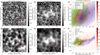 |
Fig. 9. Same as Fig. 3, for time-averaged dataset. |
| In the text | |
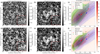 |
Fig. 10. Same as Fig. 4, for time-averaged dataset. |
| In the text | |
|
Fig. 11. Time-averaged ALMA Band 3 brightness temperature for the same measurement set as used by Molnar et al. (2019), i.e. ADS/NRAO.ALMA#2016.1.01129.S from 23 April 2017. The data were averaged over the period from 17:31 to 17:41 UTC. (a) The whole FOV. (b) The central 24 Mm × 24 Mm part, also indicated by the red box in panel (a) for comparison with the simulated data. |
| In the text | |
|
Fig. 12. Same as Fig. 9, for the Molnar et al. (2019) definition of linewidth. The black dashed line denotes the linear fit by Molnar et al. (2019). |
| In the text | |
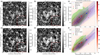 |
Fig. 13. Same as Fig. 12, for 0.8 mm. |
| In the text | |
|
Fig. 14. Same as Fig. 7, but for the time-averaged data set, for the Molnar et al. (2019) definition of linewidth. The legend is the same as for Fig. 7 |
| In the text | |
|
Fig. 15. Same as Fig. 8, but for the time-averaged data set, for the Molnar et al. (2019) definition of linewidth. |
| In the text | |
|
Fig. 16. Simulated logarithmic gas temperature (grey-scale) in a vertical slice of 3D rMHD Bifrost simulations. The solid lines represent the heights at which the optical depth is unity at a wavelength of 3.2 mm (red), and 0.8 mm (green), which correspond to ALMA bands 3, 5 and 7, respectively. The orange, white and yellow lines show the average heights at which the red and blue sides of the Hα line width according to the Leenaarts et al. (2012), Molnar et al. (2019) and FWHM definitions of linewidth are formed. |
| In the text | |
|
Fig. 17. Maps of linewidths for original resolution case for the single snapshot: Left: Leenaarts et al. (2012) definition, middle: Molnar et al. (2019) definition and right: FWHM. |
| In the text | |
|
Fig. 18. Left: Distribution of Hα line core widths (following the definition by Leenaarts et al. 2012) for the whole time series. Right: Corresponding line widths according to the definition by Molnar et al. (2019). The whole box, QS and EN regions are separately plotted in blue, black and red, and mean and median values for the three sets of pixels are indicated with a dot-dashed and dashed lines in the respective colours. Please note the difference in ranges for linewidths axes in the two plots. |
| In the text | |
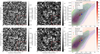 |
Fig. A.1. Same as Fig. 3, but for 0.4 mm corresponding to ALMA Band 9-10. |
| In the text | |
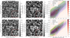 |
Fig. A.2. Same as Fig. 3, but for 0.7 mm corresponding to ALMA Band 8. |
| In the text | |
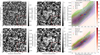 |
Fig. A.3. Same as Fig. 3, but for 1.0 mm, corresponding to ALMA Band 7. |
| In the text | |
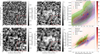 |
Fig. A.4. Same as Fig. 3, but for 2.0 mm, corresponding to ALMA Band 4. |
| In the text | |
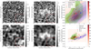 |
Fig. A.5. Same as Fig. 3, but for 3.6 mm, corresponding to ALMA Band 3. |
| In the text | |
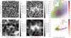 |
Fig. A.6. Same as Fig. 3, but for 4.5 mm, corresponding to ALMA Band 2. |
| In the text | |
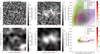 |
Fig. A.7. Same as Fig. 3, but for 6.5 mm, corresponding to ALMA Band 1. |
| In the text | |
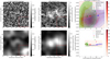 |
Fig. A.8. Same as Fig. 3, but for 8.5 mm, corresponding to ALMA Band 1. |
| In the text | |
Current usage metrics show cumulative count of Article Views (full-text article views including HTML views, PDF and ePub downloads, according to the available data) and Abstracts Views on Vision4Press platform.
Data correspond to usage on the plateform after 2015. The current usage metrics is available 48-96 hours after online publication and is updated daily on week days.
Initial download of the metrics may take a while.