| Issue |
A&A
Volume 673, May 2023
|
|
|---|---|---|
| Article Number | A21 | |
| Number of page(s) | 13 | |
| Section | Stellar atmospheres | |
| DOI | https://doi.org/10.1051/0004-6361/202245206 | |
| Published online | 27 April 2023 | |
Synthetic photometry for carbon-rich giants
V. Effects of grain-size-dependent dust opacities★
1
Theoretical Astrophysics, Department of Physics and Astronomy, Uppsala University,
Box 516,
75120
Uppsala,
Sweden
e-mail: This email address is being protected from spambots. You need JavaScript enabled to view it.
2
Department of Astrophysics, University of Vienna,
Türkenschanzstrasse 17,
1180
Vienna,
Austria
Received:
11
October
2022
Accepted:
25
February
2023
Abstract
Context. The properties and the evolution of asymptotic giant branch (AGB) stars are strongly influenced by their mass loss through a stellar wind. This, in turn, is believed to be caused by radiation pressure due to the absorption and scattering of the stellar radiation by the dust grains formed in the atmosphere. The optical properties of dust are often estimated using the small particle limit (SPL) approximation, and it has been used frequently in modelling AGB stellar winds when performing radiation-hydrodynamics (RHD) simulations.
Aims. We aim to investigate the effects of replacing the SPL approximation by detailed Mie calculations of the size-dependent opacities for grains of amorphous carbon forming in C-rich AGB star atmospheres.
Methods. We performed RHD simulations for a large grid of carbon star atmosphere+wind models with different effective temperatures, luminosities, stellar masses, carbon excesses, and pulsation properties. Also, a posteriori radiative transfer calculations for many radial structures (snapshots) of these models were done, resulting in spectra and filter magnitudes.
Results. We find that, when giving up the SPL approximation, the wind models become more strongly variable and more dominated by gusts, although the average mass-loss rates and outflow speeds do not change significantly; the increased radiative pressure on the dust throughout its formation zone does, however, result in smaller grains and lower condensation fractions (and thus higher gas-to-dust ratios). The photometric K magnitudes are generally brighter, but at V the effects of using size-dependent dust opacities are more complex: brighter for low mass-loss rates and dimmer for massive stellar winds.
Conclusions. Given the large effects on spectra and photometric properties, it is necessary to use the detailed dust optical data instead of the simple SPL approximation in stellar atmosphere+wind modelling where dust is formed.
Key words: stars: AGB and post-AGB / stars: carbon / stars: winds, outflows
Full Table C.1 is only available at the CDS via anonymous ftp to cdsarc.cds.unistra.fr (130.79.128.5) or via https://cdsarc.cds.unistra.fr/viz-bin/cat/J/A+A/673/A21
© The Authors 2023
 Open Access article, published by EDP Sciences, under the terms of the Creative Commons Attribution License (https://creativecommons.org/licenses/by/4.0), which permits unrestricted use, distribution, and reproduction in any medium, provided the original work is properly cited.
This article is published in open access under the Subscribe to Open model. This email address is being protected from spambots. You need JavaScript enabled to view it. to support open access publication.
1 Introduction
Asymptotic giant branch (AGB) stars are in complex, very late evolutionary stages as descendents of stars that started their lives on the main sequence with masses of ~0.8–8 M⊙. They mainly generate energy in a H-burning shell, interrupted by periods of intense He-burning in an inner shell during the so-called He-shell-flashes (see, e.g. Herwig 2005 for details). Many of the AGB stars are variable in brightness (as Mira stars or other types of long-period variables, LPVs) – this has often been interpreted as pulsations, especially for Miras. Another important point is the chemical evolution of the stellar atmosphere when the products of nucleosynthesis are dredged-up to the surface through the deep convection zone; in particular, the carbon produced by He burning may turn an M-type AGB star into a carbon star if/when the atmospheric abundance of carbon exceeds that of oxygen.
The evolution of stars in the AGB stage is more determined by mass loss from the surface than by the growth of their cores. The mass loss from AGB stars has been the subject of research for at least the past 60 yr, both observationally and theoretically (see, e.g. the review by Höfner & Olofsson 2018). One popular mass-loss scenario is the pulsation-enhanced dust-driven outflow, where the stellar pulsations generate outward shocks that carry material to higher and cooler layers where dust can condense; the opacity of the dust causes the material to experience a radiation pressure that can, under suitable conditions, induce and sustain a stellar wind.
This scenario has been modelled theoretically with the radiation-hydrodynamics code DARWIN (see Höfner et al. 2016, and below) and resulting synthetic observables have been presented in a series of papers. In the first article in this series, Aringer et al. (2009, hereafter Paper I) calculated spectra and photometric indices for hydrostatic carbon star photospheric models. Nowotny et al. (2011, hereafter Paper II), found that including a pulsating atmosphere and dust formation in the wind produced observables largely in agreement with those of the carbon star RU Vir. Nowotny et al. (2013, hereafter Paper III) presented a sequence of carbon star atmosphere and wind models with varying parameters to illustrate the properties of early to late carbon stars. In the previous article in this series (Eriksson et al. 2014, hereafter Paper IV), we calculated synthetic colours and spectra for a large grid of solar-metallicity carbon star atmosphere and wind models. The mass-loss rates of these models, together with other DARWIN results presented by Mattsson et al. (2010) and Bladh et al. (2019), were used by Pastorelli et al. (2019, 2020) in their population synthesis studies of SMC and LMC AGB stars, demonstrating the critical role of a realistic mass-loss description.
Photometric observational data, both in the form of long time series for individual AGB stars (e.g. Whitelock et al. 2006; Menzies et al. 2006) and large surveys (e.g. Soszyński et al. 2009; Groenewegen et al. 2020), has played an important role in studying the stellar pulsations, and their effects on the dust-forming atmospheres. While high-angular-resolution techniques have made it possible to resolve the atmospheres and wind formation zones of a handful of nearby AGB stars (e.g. Sacuto et al. 2011; Khouri et al. 2016; Wittkowski et al. 2017), photometry is still a critical tool for studying large samples with different stellar parameters. As these stars are very luminous they can be observed also in other galaxies. In addition, large spectroscopic surveys, combined with efficient spectral classification methods, can contribute to our understanding of evolved stars (e.g. Li et al. 2018).
In the present paper, we improve on our earlier calculations, using dust opacities that depend on the size of the dust grains, in contrast to Paper IV where we assumed the small particle limit (SPL) for the dust opacity. The current study was motivated by our previous results, showing that grains tend to reach sizes beyond the regime where the SPL applies. We find that the mass-loss rates and outflow velocities are similar to the previous results, but the dust condensation (and thus the dust-to-gas ratio) is much smaller, and the photometric filter magnitudes and colours are also quite strongly affected.
2 Dynamic models and radiative transfer
The modelling of dynamic structures and synthetic observables follows the general approach described in Papers II–IV of this series. Here, we only give a brief summary, referring the reader to these and other papers for a more comprehensive description. A more detailed description of the size-dependent dust opacities used here, in contrast to Papers II–IV, is given below.
2.1 Dynamic atmosphere and wind models
The time-dependent radial structures of atmospheres and winds are produced by simultaneously solving the equations of hydrodynamics, frequency-dependent radiative transfer, and non-equilibrium dust formation (describing nucleation and growth of amorphous carbon grains) using the DARWIN code (see Höfner et al. 2003, 2016). Each dynamic model is represented by a sequence of snapshots of radial structures, typically covering hundreds of pulsation periods. Wind properties are derived from the time sequences as described in Sect. 3.1.
The computation of a dynamical model starts from a hydrostatic, dust-free configuration characterized by the fundamental stellar parameters (mass, luminosity, effective temperature) and abundances of chemical elements, which is comparable to classical model atmospheres. The effects of stellar pulsation are simulated by time-dependent boundary conditions at the inner edge of the computational domain, located just below the stellar photosphere. The velocity of the innermost mass shell is prescribed as a sinusoidal variation with the period and amplitude as parameters (so-called piston model), and the amplitude of the accompanying luminosity variation can be adjusted separately (see Appendix B in Höfner et al. 2016).
2.2 Grain-size-dependent opacities
As mentioned above, the dynamical models presented here differ from those in Paper IV by the treatment of dust opacities. The total opacity (cross-section/mass) at wavelength λ of an ensemble of spherical dust grains with radii, agr, embedded in a gas of mass density ρ, can be expressed as
 (1)
(1)
where n(agr) dagr is the number density of grains in the size interval dagr around agr, and Q(agr, λ) is the efficiency factor, defined as the radiative cross-section C(agr, λ) divided by the geometrical cross-section of the grains, that is
 (2)
(2)
In the DARWIN code, the properties of carbon dust, at distance from the centre of r and a time of t, are described by moments of the grain size distribution, weighted with powers of the grain radius:
 (3)
(3)
where K0 is proportional to the total number density of grains (the integral of the size distribution function over all grain sizes), K1 is related to the average grain radius, and K3 to the average volume of the grains, respectively.1 By introducing the quantity Q′ = Q/agr, we can re-write Eq. (1) as
 (4)
(4)
where the integral, apart from the factor Q′(agr, λ) looks similar to the definition of moment K3.
For grains that are much smaller than the wavelength under consideration, the small particle limit (SPL) of Mie theory gives Qabs ∝ agr and  for the absorption and scattering efficiencies, respectively. In this case,
  is independent of the grain radius, and the integral over grain size can be represented by moment K3 of the size distribution, while the scattering efficiency becomes negligible. The assumption of SPL has been used in many dust-driven wind models found in the literature, including Papers II–IV. As it turned out, however, the resulting grain sizes may be well beyond the range where the SPL is valid.
For grains that are of sizes comparable to the wavelengths under consideration, the quantity Q′ depends on the grain radius in a complex way, and can be computed numerically from full Mie theory. Assuming that the grain sizes at each point in the model are well-represented by the average grain radius 〈agr〉 (derived from moment K1 of the size distribution), we can re-formulate Eq. (4) as
 (5)
(5)
In the models presented in this paper, the efficiency factors for absorption and scattering, as well as the mean scattering angle required for calculating the radiative pressure, are computed using Mie theory for spherical particles (programme BHMIE by B.T. Draine2) and optical properties of amorphous carbon by Rouleau & Martin (1991). The efficiency factor, Qacc(agr, λ), representing radiative pressure contains contributions from true absorption and scattering, that is
 (6)
(6)
where gsca is an asymmetry factor describing deviations from isotropic scattering. Examples of efficiency factors and their dependence on grain size and wavelength are shown in Fig. 1, demonstrating the limitations of the SPL assumption, used in earlier models.
 |
Fig. 1 Efficiency factors as a function of grain size for an amC particle computed with full Mie theory (lines dashed red: absorption; dash-dotted blue: scattering; black: radiative pressure) and in the SPL approximation (absorption, plus signs). Top panel: values at a wavelength of 0.54 μm (V band). Bottom panel: values at a wavelength of 2.1 μm (K band; see text for details). While scattering is negligible in the SPL, it contributes significantly to the radiation pressure for particles with sizes that are comparable to the wavelength. |
2.3 Stellar and pulsation parameters
The models have fundamental parameters (effective temperature, luminosity, and stellar mass) as given in Table 1. The stellar parameter combinations in the present grid are the same as in Paper IV. All models have solar abundances following Asplund et al. (2005), except for the carbon abundance. The values are given on the scale where log NH ≡ 12.00. The abundances from Asplund et al. (2005) correspond to a composition by mass: X/Y/Z = 0.73/0.25/0.015–0.020; the variation being due to the varying carbon abundance. For every combination of stellar parameters in the table, models were computed with carbon excesses of log(C–O) + 12 = 8.2, 8.5 and 8.83 and with piston velocity amplitudes of ∆up = 2, 4 and 6 km s−1. The pulsation periods are given by the luminosity through a period-luminosity relation following Feast et al. (1989); for easy reference, the periods are also given in Table 1, although they are not treated as an independent parameter4.
During a pulsation cycle, the radius of the innermost mass shell of the model and the luminosity at that position vary simultaneously, simulating a coupling between the variable brightness and size of the star. Without a quantitative model of the pulsating stellar interior, assumptions have to be made about the forms, the amplitudes, and the relative phases of these temporal variations. Regarding the dynamic boundary (i.e. gas velocity), the functional form is of minor importance since the outward-travelling waves quickly develop into shocks and the kinetic energy transferred into the atmosphere is mostly determined by the velocity amplitude. Therefore, we adopted the common assumption of a sinusoidal variation, parametrised by the velocity amplitude, ∆up and the pulsation period, P. In this differential study of the influence of size-dependent dust opacity, we keep the choice of Paper IV and assume that the luminosity at the position of the innermost mass shell varies in phase with its radius and that the amplitude of the luminosity variation is correlated with the radius amplitude. An adjustable factor, fL, was introduced (see Nowotny et al. 2010, for details) to scale the luminosity variations. Paper IV varied the value of this parameter and found no significant changes in the dynamic properties, so we kept their choice of fL = 2.
Combinations of fundamental stellar parameters covered by the model grid.
Relation between the carbon excess measure log(C–O) + 12 and the C/O ratio for the adopted chemical composition (Asplund et al. 2005), i.e. using an oxygen abundance of log(NO/NH)+12 = 8.66.
2.4 Synthetic spectra and photometry
For each combination of stellar and pulsational parameters, snapshots of the atmospheric structures at various phases (typically 20 per period) during several consecutive periods (typically four) and for a few different epochs during the simulation time span were used for the detailed a posteriori radiative transfer calculations. We need more than one period to obtain a representative behaviour since the models are not strictly periodic, mainly due to the time-dependent dust formation. We applied the code COMA (Aringer 2000, and Paper I), version 11, to compute atomic, molecular, and amorphous carbon (amC) dust. While Eriksson et al. (2014) used dust opacities calculated under the assumption of the small particle limit, here we used size-dependent opacities based on Mie theory and amC optical properties from Rouleau & Martin (1991). We note that the treatment of the opacities is consistent with that in the generation of the dynamic models, except for a higher spectral resolution in the a posteriori radiative transfer calculations (10000).
The resulting synthetic spectra in the 0.35–25 μm wavelength range were used to compute filter magnitudes in the Johnson-Cousins BVRI system (Bessell 1990) and the Johnson-Glass JHKLL′M system (Bessell & Brett 1988). More details can be found in previous articles, for example Paper II. The results given in the table in Appendix C include a temporal mean of the V and K magnitudes, as well as their (maximum) ranges, and also the mean values of the colours (V–I), (V–K), (J–H), and (H–K).
3 Effects of size-dependent dust opacities
In this section, we describe the resulting differences between models using size-dependent dust opacities (SDDO) and the SPL assumption. We mainly discuss the changes of time-averaged properties, giving an overview of trends for the whole grid. In some cases, we show the time-dependent behaviour of individual models in order to demonstrate the underlying physical mechanisms.
3.1 Dynamical and dust properties
The resulting dynamic properties of the new SDDO models are compiled in the table in Appendix C. The listed values are time-averages of the mass-loss rates, outflow velocities, and carbon condensation degrees, and these were determined in the following way. For a given model, the existence of a wind was defined as the outer boundary having reached 25 stellar radii and the velocity of the gas at the outer boundary being positive (i.e. an outflow). Then, for each (pulsation) cycle with the wind condition fulfilled, the mass-loss rate and so on were determined, and later means and standard deviations were calculated. For most models, several hundred cycles were used to determine the means. For some combinations of fundamental parameters, a wind is sustained only for limited periods, resulting in episodic behaviour. In this paper, we define a model as episodic when wind conditions prevail for more than 15% but less than 85% of the total time interval (after the first instance of wind conditions).
In general, mass loss is favoured by low T★ (easier to form dust at cooler temperatures), high luminosity (more momentum transferred from radiation to dust grains), small stellar mass (shallower potential well), large (C–O) (more free carbon to form amorphous carbon grains), and a large piston velocity amplitude (stellar layers reach out to a greater distance from the centre of the star during pulsations). In total, 268 different dynamic model atmospheres were computed (96 of them produced winds and 172 did not lead to outflows). For the SPL case, the corresponding numbers are 95 with outflows and 173 without. An overview of the wind or no-wind status of the different models can be given in so-called wind maps, where the status of a model (no-wind/episodic/wind) is shown in an HR-diagram-like representation. Wind maps of the current grid (SDDO, with size-dependent dust opacities) and the SPL grid are displayed in Fig. 2. As seen, the qualitative changes in dynamic behaviour are minor, mostly consisting of changes from/to the episodic cases.
The relatively small effects on the mass-loss rates and on the outflow velocities when we replace SPL by SDDO are clearly seen in the upper two panels of Fig. 3, where the new (SDDO) values are plotted against the SPL ones. For some model parameter combinations and borderline cases, the wind turns on and off one or more times during the simulation sequence(s); these episodic cases are plotted as triangles where one or both of the models display this behaviour. As seen, it is only these episodic cases that exhibit large differences in mass-loss rates between SPL and SDDO. We note the expected trend of higher outflow speeds for the larger values of the carbon excess (more dust giving more acceleration to the flow).
With SDDOs, the carbon condensation degrees and grain sizes are smaller than for the SPL models. This is seen in Fig. 3 for all non-episodic models producing winds. The condensation degree of carbonaceous dust, and hence the dust-to-gas ratio, is roughly half as big in the SPL case. We note that the dust grains do not grow so large as they quickly travel through the dust formation regions, which is a consequence of higher radiative force compared to the SPL case (see Fig. 1). The largest grains grow in the slow outflows in models with small carbon excesses, especially for the episodic cases.
The change in dust opacity from SPL to SDDO causes changes in the time-dependent behaviour of the models. This is visualised in Fig. 4 for some models with stellar masses of 0.75 M⊙ and for some models with masses of 1.5 M⊙ in Fig. 5, where the (gas) density at the outer boundary for 50 consecutive periods are displayed. We see the same general behaviour for all cases: a larger density contrast in the wind for the SDDO models as compared to the SPL ones, that is a wind with narrower and more pronounced gusts of gas and dust. This is probably a consequence of the steeper dependence of radiative acceleration on the size of the growing grains in the SDDO case (see Fig. 1).
In summary, the mass-loss rates and outflow speeds are not strongly affected by replacing the SPL approximation with SDDOs. The higher radiative force on sub-micron-sized dust grains, compared to the SPL case, however, tends to result in smaller dust grains and lower condensation degrees. These general trends in wind properties are in good agreement with the results of a pilot study by Mattsson & Höfner (2011), which is based on a much smaller number of DARWIN models than in the current grid.
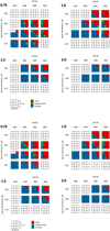 |
Fig. 2 Dynamic behaviour of models these are also referred to as wind-maps. In an HR-type display, the models are colour-coded as red for wind, blue for no wind, and green for episodic behaviour. The upper four panels show the SDDO case and the lower four show the grid with the SPL approximation. The four sub-panels for each grid show models of different stellar masses indicated in the top left corner. For each given combination of temperature and luminosity, the different carbon excesses and piston amplitudes are arranged as shown in the bottom legend. |
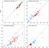 |
Fig. 3 Comparison of different properties of SDDO versus SPL grids. The quantities plotted are mass-loss rates (upper left), outflow speeds (upper right), condensation degrees (lower left) and dust grain radii (lower right). The different carbon excesses are shown in colour: log(C-O) = 8.2 in green, 8.5 in blue, and 8.8 in red. Circles denote wind models and triangles denote episodic models. |
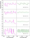 |
Fig. 4 Gas density at outer boundary as a function of time for selected models with a stellar mass of 0.75 M⊙. The left column displays the SDDO values, the right one the SPL values. Stellar parameters, Teff, log L, carbon excess class and piston amplitude, are given in the SPL panels. The densities are given in cgs units: Teff in K, log L in L⊙, and piston amplitudes in km s−1. We use a fixed range in gas density in all panels. |
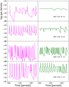 |
Fig. 5 Gas density at the outer boundary as a function of time for 1.5 M⊙ models (see Fig. 4 for details). |
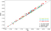 |
Fig. 6 Mean K magnitude for models in the entire grid computed without using the dust opacity in the a posteriori radiative transfer (COMA). The values for the SDDO cases versus the SPL ones are plotted. |
3.2 Photometric properties
Going from SPL to SDDO, the photometric magnitudes could change due to the direct effects of the different dust opacities or through the indirect effects on the structures of the atmosphere+wind caused by the dust. The effects due to changes in the structures can be estimated by computing spectra without taking opacity from the dust into account. We find that the impacts of structural changes are minor for all filters (≲0.1 mag); Fig. 6 shows a comparison of the K magnitudes.
An overview of the differences in the photometric properties with SDDOs compared to SPL models is shown in Fig. 7, displaying the mean V, J, H, and K magnitudes for the models in the entire grid (wind and no-wind models). The K magnitude is typically brighter by 0.2–0.4 magnitudes for the wind models with SDDO. This is mainly due to the reduced amount of dust (lower condensation degree) in the SDDO models (see Fig. 3). The H magnitudes for the wind models are also generally brighter without SPL, typically by 0.5 magnitudes. From the J magnitude to shorter wavelengths, the influence of dust is more complex; for small dust veiling the value is smaller (i.e. brighter), but for increasing obscuration the magnitudes are fainter for the SDDO models, in V by up to three magnitudes. As seen in the figure, this occurs primarily for the highest carbon excess.
For the V band, we estimated the effect by comparing the Q value for absorption (Fig. 1, upper panel) for the smaller grains in the SDDO case with the Q value for the bigger grains in SPL models (see Fig. 3). We find that the former is almost always larger. However, for some models (mostly with a small carbon excess, C5) where the mean grain radius is larger than 0.4 μm (log agr = −4.4 cm) in the SPL case, we see in Fig. 1 (upper panel) that Q(SDDO) is smaller regardless of the SDDO grain radius. In Fig. 8, we again plot V(SDDO) versus V(SPL), now colour-coded by the value of Q(SDDO)/Q(SPL) calculated at the appropriate mean grain radii. The cases with the lowest SDDO/SPL ratios of absorption efficiency tend to show brighter mean V magnitudes. The difference in V is also dependent on the carbon condensation degree. This is shown in the right-hand panel of Fig. 8, where V is colour-coded according to the ratio of the mean condensation degree in the SDDO model to that in the SPL model. As expected, a lower relative amount of dust correlates well with brighter mean V magnitudes. In summary, the behaviour of the V magnitude in Fig. 7 is the result of the combined effects of changed Q values and different condensation degrees, as illustrated in Fig. 8.
Turning from the mean magnitudes to the time-variations, that is, the light curves, we show some examples in Fig. 9 and Fig. 10. To illustrate the photometric variations, we chose two models in Fig. 5 with different characteristics: one with a smaller carbon excess and pulsation amplitude, the other with larger values for these properties; otherwise, the models have the same fundamental parameters. In Figs. 9 and 10, we show the light-curves in V, J, and K as well as the two-colour diagram for (J–H) versus (H–K) for the two models, for both SDDO and SPL. We note period-to-period variations that are larger at visual compared to near-infrared (NIR) wavelengths. The same is true for epoch-to-epoch variations. For high-mass-loss models (such as in Fig. 10), the influence of dust may lead to less periodic variations in V.
We refer to the difference between maximum and minimum brightness during a period as the amplitude, while the difference during all the computed epochs is referred to as the range. We find that the range in K can be larger by up to 0.5 magnitudes for the highest mass-loss SDDO models with much dust in their winds (see Fig. 11). Also, two episodic C5 models show large ranges in the SDDO case due to strong epoch-to-epoch variations.
Plotting the V magnitude amplitudes and ranges for the SDDO versus the SPL grid (Fig. 12), we see the same pattern as for the mean V magnitude itself, as discussed above: smaller amplitude or range and a brighter mean value for moderate mass-losing models, while models with heavy mass loss show larger variations and a fainter mean value when the SPL assumption is replaced by SDDO. Comparing the left and right panels in Fig. 12, some models show much larger ranges in long-term variation than the amplitude over a period; this reflects gusts of dust occurring now and then, extending the range of variations in V. We also note, as we show in Fig. 7, that the V magnitudes are smaller (brighter) for the lower carbon excesses and the C6 models and have smaller amplitudes.
A further examination of the results of the radiative transfer calculations done with COMA is provided in the appendix. The optical depth as a function of distance to the stellar surface, for a maximum phase in the model in Fig. 10, are shown in Figs. A.1 and A.2 for SDDO and SPL, respectively. We draw the reader’s attention to how far from the star the light in for instance the V band originates for models with a large carbon excess.
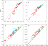 |
Fig. 7 Mean V, J, H, and K magnitude for models in the entire grid. The values for the SDDO cases versus the SPL ones are plotted. Colours and symbols are explained in Fig. 6. |
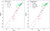 |
Fig. 8 Mean V magnitude for wind models in the SDDO versus SPL cases. In the left panel, the points are colour-coded according to Q(SDDO)/Q(SPL) and evaluated at appropriate grain radii. In the right panel, the colour is given by the ratio of the mean condensation degree in the SDDO and the SPL cases. |
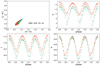 |
Fig. 9 Photometrie variations of the models shown in the top row of Fig. 5. The (J–H) versus (H–K) diagram (top left) and the light curves of the V (top right), J (bottom left), and K (bottom right) magnitudes for three periods in several epochs. The SDDO values are plotted in orange-red hues, and the SPL values are plotted in blue-ones. The model has the parameters Teff = 2600 K, log L = 4.0 L⊙, mass 1.5 M⊙, log(C–O) = 8.5, and a piston amplitude of 4 km s−1. |
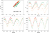 |
Fig. 10 As Fig. 9, but for the models with log(C–O) = 8.8 and piston amplitude of 6 km s−1 (bottom row in Fig. 5). |
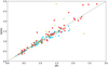 |
Fig. 11 Mean range in K magnitudes for models in the entire grid. The SDDO values are plotted versus the SPL ones. Colours and symbols are explained in Fig. 6. |
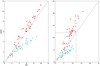 |
Fig. 12 Mean amplitude in V magnitudes (left) and their range (right) for models in the entire grid. The SDDO values are plotted versus the SPL ones. The models are colour-coded according to their carbon excess (see Fig. 6). In the right panel, the area of the left panel is outlined. |
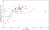 |
Fig. 13 Mass-loss rates versus outflow speeds for wind models in the grid for the SDDO case. The different colours denote the carbon excess. Colours and symbols are explained in Fig. 6. Observational data from Schöier & Olofsson (2001) and Ramstedt & Olofsson (2014) are plotted as grey symbols. |
4 Comparisons to observational data
In this section, we compare the new results to several observational studies of carbon stars. One useful way of displaying the dynamic properties of a grid is to plot the mass-loss rates versus the outflow speeds. Both quantities can be estimated from millimetre-wave observations of CO rotational lines and radiative transfer modelling of these lines. For the SDDO models, such a diagram is shown in Fig. 13, and this can be compared to Fig. 4 in Paper IV for the SPL case. As noted in Sect. 3.1, these quantities do not change much when SPL is replaced by SDDO. In Fig. 13, we display these quantities from the present grid and observations of carbon stars given by Schöier & Olofsson (2001) and Ramstedt & Olofsson (2014) with updated values for sources in common. We note a general agreement, but find some models with very high outflow speeds not seen in these observations. Also, some models with low outflow speeds and rather high mass-loss rates lack observed counterparts. We highlight, however, that not all parameter combinations in the computed grid necessarily occur in nature, or they may be very rare or just not yet observed. In summary, it appears that the models with a moderate carbon excess (C6) show a trend and values of mass-loss rates and wind velocities that agree best with the observations.
The two-colour diagram, (J–H) versus (H–K), is commonly used to compare models to observations. In Fig. 14, we show this diagram for the SDDO models using coloured symbols and for the SPL ones (originally shown in Fig. 13 in Paper IV in grey tones, together with observational data from Whitelock et al. (2006). The slope in the diagram is steeper for the SDDO grid than for the SPL one. This is mostly due to (J–H) becoming larger for SDDO models: H gets brighter more than J does (if at all; see Sect. 3.2, as well as Appendix A). Thus, we note that this slope depends on the details of the dust opacities.
Comparing the SDDO grid to the photometric near-infrared observations by Whitelock et al. (2006), we used the data in their Table 6 where de-reddened J, H, and K magnitudes are listed. Also, some data from their Table 3 are included in our comparison, namely for sources with K < 4, which can be assumed not to be significantly reddened by interstellar extinction. The colours for the SDDO grid agree with observations rather well for 1.0 ≲ (H–K) ≲ 1.5 (i.e. the range of moderately dusty winds). For (H–K) ≳ 1.5, we find SDDO models with low effective temperatures, high luminosities, large carbon excess (C7) and high mass-loss rates, typically 10−5 M⊙yr−1, very red (J–K) colours (≳ 4), and high levels of dust (gas-to-dust ratios ~500–800; see below). Different variability classes for the observed stars are plotted with different colours. The non-Mira stars in Whitelock et al. (2006) fit less well, especially for (H–K) ≲ 1.0; in this interval, updated gas opacities for the models could improve the agreement.
As an example, in Fig. 15 we show a (J–H) versus (H–K) diagram for dust-free hydrostatic carbon star models from Aringer et al. (2016, 2019). The models are computed with the COMARCS code and a have solar metallicity of log(g [cm s−2]) ≤ 0.0, effective temperatures down to 2500 K, and different masses. Two different C/O values are used: 1.4 and 2.0 (here, only the abundance of carbon is changed with respect to a solar mixture). For each C/O value, two sets of models are shown: the original ones and a set with updated gas opacities. For C2, data by Querci et al. (1974) is replaced by Yurchenko et al. (2018); McKemmish et al. (2020), and for C2H2, data from Jorgensen et al. (1989) is replaced by Chubb et al. (2020). The large differences between the two sets of models are due to differences of these gas opacities. In the figure, we also plot observational values for carbon stars selected to be little influenced by dust. The observational values come from Bergeat et al. (2001); Cohen et al. (1981); Costa & Frogel (1996); Gonneau et al. (2016); Totten et al. (2000); Gullieuszik et al. (2012) and agree much better with the set of hydrostatic dust-free models with the updated gas opacities.
The grey box in Fig. 14 centred at (0.5, 1.0) outlines the ranges covered by Fig. 15, indicating that the inclusion of updated C2 and C2H2 gas opacities in future hydrodynamic DARWIN models should improve the agreement with observations for nearly dust-free models. In the current paper, focussing on dust opacities, however, we chose to keep the same set of gas opacity data as in Paper IV to make the SPL and SDDO grids comparable in that respect.
In the colour-magnitude diagram (Fig. 16) displaying MK versus (J–K)0, the observed values from Whitelock et al. (2006), Table 6, come from de-reddened magnitudes and a bolometric PL relation for LMC to derive distances and bolometric corrections. For northern sources, we used the values in Menzies et al. (2006), Table 3, to calculate MK and (J–K)0. We see that the values from our SDDO grid bracket the observed values for (J–K)0 ≲ 4, while the redder stars seem to be affected by larger cŕrcumstellar extinction in K than the models in our grid.
The distribution of carbon stars in colour-magnitude diagrams is relatively flat, which makes them potential candidates as standard candles for (extragalactic) distance determinations, especially as they are intrinsically very bright. This was first studied by Richer et al. (1984), who used VRI photometry to estimate the distance to NGC 205, and later by Weinberg & Nikolaev (2001), who calibrated the MJ versus (J–Ks) distribution of carbon stars in a narrow range in (J–Ks) from 2MASS photometry of the Magellanic Clouds. Recently, this so-called JAGB method has been used for distance determinations by Ripoche et al. (2020) and simultaneously by Freedman & Madore (2020) and in later publications by these groups. Here stars in a population with 1.4 < (J–Ks) < 2.0 are assumed to be carbon stars with a well-determined MJ of −6.2. The precision of this method depends on selection effects in the samples of calibrators, for example the metallicity (as discussed by Lee et al. 2021). In Fig. 17, we show the mean MJ versus (J–Ks)0 for the SDDO grid, and we note a general similarity to Fig. 1 of Madore et al. (2022). In all magnitude-limited samples, one suffers from a Malmquist bias, and Parada et al. (2021) discussed the advantage of using median instead of mean magnitudes for stars in extragalactic surveys. There might also be a difference in our grid between the median and mean magnitudes derived from the light curves. As presented in Appendix B, we find that the median magnitude is generally somewhat brighter than the mean one, but this effect is only significant for some models with the highest carbon excesses (C7). This is due to asymmetric light curves (an effect of very gusty winds). The effect on the J magnitude is mostly much smaller than 0.2 magnitudes. For reasons of comparability with earlier papers and with the SPL grid, we therefore used mean magnitudes for the SDDO models in the figures discussed in this section.
The mass-loss rates for the SDDO models are plotted as a function of the (J–K)0 colour in Fig. 18. For comparison, corresponding values given by Whitelock et al. (2006) are shown. These are derived from the 60 μm IRAS fluxes (assumed to originate from dust in the cŕrcumstellar envelopes) using an expression from Jura (1987). Mass-loss rates by Schöier & Olofsson (2001) and Ramstedt & Olofsson (2014) from CO data are also plotted. We find a reasonable general agreement between models and observations given the underlying uncertainties. In particular, when comparing with the mass-loss rates given by Whitelock et al. (2006), we must remember that these values are based on Jura (1987), who used a gas-to-dust ratio of 220 to convert the dust-mass-loss rates into total mass loss. This ratio is considerably lower than in our models (see Fig. 19). We find values of the order of 103 for our grid of models, reflecting typical condensation degrees well below 1 (see Fig. 3). These gas-to-dust values are considerably higher than those often assumed in the literature.
Taking the mass-loss rates in Whitelock et al. (2006) and their value for the gas-to-dust ratio adopted from Jura (1987), we calculated the dust-mass-loss rates in their sample. These are plotted in Fig. 20, together with the dust-mass-loss rates for the SDDO grid. We note a better agreement between model values and those derived from observations than for the total mass-loss rates (Fig. 18). For (J–K) ≳ 4, however, the models tend to have lower mass-loss rates at a given (J–K). This is interesting in light of the discrepancies in the colour-magnitude diagram (Fig. 16) in the same (J–K) range.
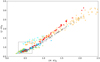 |
Fig. 14 Mean (J–H) colour versus mean (H–K) colour for models in the entire grid. Models using SPL are plotted in grey tones, and those with SDDO are coloured according to carbon excess (see Fig. 6). Observed carbon stars from Whitelock et al. (2006) are also plotted: orange symbols for Miras and cyan for non-Mira stars. The grey box centered at (0.5, 1.0) outlines the area in Fig. 15. |
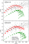 |
Fig. 15 (J–H) versus (H–K) for hydrostatic dust-free carbon star models from the COMARCS grid presented in Aringer et al. (2016, 2019, green squares). Two C/O ratios are shown: 1.4 and 2.0. The results are compared to a similar grid computed with updated opacities for molecular and atomic transitions (red circles). The large shift between the two sets of models is due to changes of the absorption caused by C2 and C2H2. In addition, observed values of carbon stars are included (crosses); they cover objects with solar and subsolar metallicities (see text). |
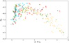 |
Fig. 16 MK values versus mean (J–K)0 colour for SDDO models in the entire grid. Colours and symbols are explained in Fig. 6. Observed carbon Mira stars from Whitelock et al. (2006) are plotted as orange symbols, and those from Menzies et al. (2006) are plotted as green symbols. |
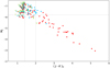 |
Fig. 17 MJ values versus mean (J–K)0 colour for the SDDO models in the entire grid. Colours and symbols are explained in Fig. 6. The value of MJ = −6.2 is marked, as well as (J–K)0 = 1.4 and 2.0. |
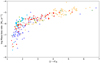 |
Fig. 18 Mass-loss rate versus mean (J–K)0 colour for the SDDO wind models in the grid. The colours denote the carbon excess (see Fig. 6), the circles with different grey hues are the SPL models. Observed carbon Mira stars from Whitelock et al. (2006) are plotted as orange symbols, while observations from Schöier & Olofsson (2001) and Ramstedt & Olofsson (2014) are plotted as blue symbols (or green if the source is also present as an orange symbol from Whitelock et al. 2006). |
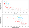 |
Fig. 19 Mean gas-to-dust ratio for the wind models in the grid plotted against the mean (J–K) colour (top panel) and against the mean mass-loss rate (lower panel). The models are colour-coded for the carbon excess (see Fig. 6). For models computed with the SPL, we use grey symbols. |
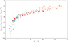 |
Fig. 20 Mean dust-mass-loss rate versus mean (J–K)0 colour for the wind models in the grid. The observed dust-mass-loss rates (plotted as orange symbols) were derived from total mass-loss rates in Whitelock et al. (2006) using a gas-to-dust ratio of 220. |
5 Summary and conclusions
Carbonaceous dust is crucial for driving the stellar winds in carbon stars, and the mass loss will eventually terminate their evolution along the AGB. We computed grids of dynamical atmosphere and wind models representing these stars in order to investigate the effects of changing the dust opacity from the simple small particle approximation (SPL) to a size-dependent treatment using Mie calculations. The grids include 268 combinations of physical parameters appropriate for C-rich AGB stars (effective temperature, luminosity, stellar mass, carbon excess, and pulsational properties). Mass loss (stellar winds) developed in about 1/3 of our radiation-hydrodynamic DARWIN models, which include time-dependent dust formation/sublimation and frequency-dependent radiative transfer. One of the main conclusions of comparing the two grids is that the mass-loss rates and outflow speeds are not strongly affected by replacing the SPL approximation with SDDOs. Due to a higher radiative force on sub-micron-sized dust grains (see Fig. 1), compared to the SPL case, they travel faster through the dust-forming outer atmosphere layers, which results in smaller dust grains and lower condensation degrees (and thus higher gas-to-dust ratios). The dynamics is tending towards more narrow and denser shells of mass loss, a more strongly variable behaviour of the winds in the new SDDO models.
We also calculated detailed a posteriori radiative transfer through the spherically symmetric radial structures for hundreds of snapshots per model using the COMA code. The resulting light curves and colour-colour diagrams, derived from the COMA flux distributions, show several differences between the SPL and the size-dependent opacity cases. Compared to SPL, we find generally brighter K magnitudes; for shorter wavelengths where the dust influence is more complex, we find brighter magnitudes when the dust absorption is small and dimmer magnitudes with large absorption, especially in the V band (all compared to the SPL case).
Some comparisons to observational data have been made, for example mass-loss rates versus outflow speeds. In Fig. 13, we compare model values to results from CO rotational line observations. Also, synthetic photometric mean magnitudes are compared to NIR observations in Fig. 14. Both these comparisons show a general agreement, but we must remember that all parameter combinations used in the model have equal weight and do not represent an observed carbon star population. Other laboratory data for the optical properties of amorphous carbon as well as the effects of using updated gas opacities should be explored in the future. We will also extend our investigations to additional photometric systems. This will primarily cover the Gaia-2MASS diagram used to identify carbon stars (e.g. Abia et al. 2022; Lebzelter et al. 2018) and mid-infrared data from different space missions (Spitzer, WISE, Akari), which contain information about the cool dust in the outer envelopes (e.g. Srinivasan et al. 2016; Nanni et al. 2018, 2019).
Acknowledgements
S.H. acknowledges funding from the European Research Council (ERC) under the European Union’s Horizon 2020 research and innovation programme (Grant agreement no. 883867, project EXWINGS) and the Swedish Research Council (Vetenskapsrådet, grant number 2019-04059). The computations were enabled by resources provided by the Swedish National Infrastructure for Computing (SNIC) at UPPMAX partially funded by the Swedish Research Council through grant agreement no. 2018-05973.
References
- Abia, C., de Laverny, P., Romero-Gómez, M., & Figueras, F. 2022, A&A, 664, A45 [NASA ADS] [CrossRef] [EDP Sciences] [Google Scholar]
- Aringer, B. 2000, Ph.D. Thesis, University of Vienna, Austria [Google Scholar]
- Aringer, B., Girardi, L., Nowotny, W., Marigo, P., & Lederer, M. T. 2009, A&A, 503, 913 [NASA ADS] [CrossRef] [EDP Sciences] [Google Scholar]
- Aringer, B., Girardi, L., Nowotny, W., Marigo, P., & Bressan, A. 2016, MNRAS, 457, 3611 [Google Scholar]
- Aringer, B., Marigo, P., Nowotny, W., et al. 2019, MNRAS, 487, 2133 [CrossRef] [Google Scholar]
- Asplund, M., Grevesse, N., & Sauval, A. J. 2005, ASP Conf. Ser., 336, 25 [Google Scholar]
- Bergeat, J., Knapik, A., & Rutily, B. 2001, A&A, 369, 178 [NASA ADS] [CrossRef] [EDP Sciences] [Google Scholar]
- Bessell, M. S. 1990, PASP, 102, 1181 [NASA ADS] [CrossRef] [Google Scholar]
- Bessell, M. S., & Brett, J. M. 1988, PASP, 100, 1134 [Google Scholar]
- Bladh, S., Eriksson, K., Marigo, P., Liljegren, S., & Aringer, B. 2019, A&A, 623, A119 [NASA ADS] [CrossRef] [EDP Sciences] [Google Scholar]
- Chubb, K. L., Tennyson, J., & Yurchenko, S. N. 2020, MNRAS, 493, 1531 [NASA ADS] [CrossRef] [Google Scholar]
- Cohen, J. G., Frogel, J. A., Persson, S. E., & Elias, J. H. 1981, ApJ, 249, 481 [NASA ADS] [CrossRef] [Google Scholar]
- Costa, E., & Frogel, J. A. 1996, AJ, 112, 2607 [NASA ADS] [CrossRef] [Google Scholar]
- Eriksson, K., Nowotny, W., Höfner, S., Aringer, B., & Wachter, A. 2014, A&A, 566, A95 [NASA ADS] [CrossRef] [EDP Sciences] [Google Scholar]
- Feast, M. W., Glass, I. S., Whitelock, P. A., & Catchpole, R. M. 1989, MNRAS, 241, 375 [NASA ADS] [CrossRef] [Google Scholar]
- Freedman, W. L., & Madore, B. F. 2020, ApJ, 899, 67 [NASA ADS] [CrossRef] [Google Scholar]
- Gonneau, A., Lançon, A., Trager, S. C., et al. 2016, A&A, 589, A36 [NASA ADS] [CrossRef] [EDP Sciences] [Google Scholar]
- Groenewegen, M. A. T., Nanni, A., Cioni, M. R. L., et al. 2020, A&A, 636, A48 [NASA ADS] [CrossRef] [EDP Sciences] [Google Scholar]
- Gullieuszik, M., Groenewegen, M. A. T., Cioni, M.-R. L., et al. 2012, A&A, 537, A105 [NASA ADS] [CrossRef] [EDP Sciences] [Google Scholar]
- Herwig, F. 2005, ARA&A, 43, 435 [NASA ADS] [CrossRef] [Google Scholar]
- Höfner, S., & Olofsson, H. 2018, A&ARv, 26, 1 [Google Scholar]
- Höfner, S., Gautschy-Loidl, R., Aringer, B., & Jorgensen, U. G. 2003, A&A, 399, 589 [NASA ADS] [CrossRef] [EDP Sciences] [Google Scholar]
- Höfner, S., Bladh, S., Aringer, B., & Ahuja, R. 2016, A&A, 594, A108 [NASA ADS] [CrossRef] [EDP Sciences] [Google Scholar]
- Ita, Y., Tanabé, T., Matsunaga, N., et al. 2004, MNRAS, 353, 705 [NASA ADS] [CrossRef] [Google Scholar]
- Jorgensen, U. G., Almlöf, J., & Siegbahn, P. E. M. 1989, ApJ, 343, 554 [NASA ADS] [CrossRef] [Google Scholar]
- Jura, M. 1987, ApJ, 313, 743 [NASA ADS] [CrossRef] [Google Scholar]
- Khouri, T., Maercker, M., Waters, L. B. F. M., et al. 2016, A&A, 591, A70 [NASA ADS] [CrossRef] [EDP Sciences] [Google Scholar]
- Lebzelter, T., Mowlavi, N., Marigo, P., et al. 2018, A&A, 616, A13 [NASA ADS] [CrossRef] [EDP Sciences] [Google Scholar]
- Lee, A. J., Freedman, W. L., Madore, B. F., Owens, K. A., & Sung Jang, I. 2021, ApJ, 923, 157 [NASA ADS] [CrossRef] [Google Scholar]
- Li, Y.-B., Luo, A. L., Du, C.-D., et al. 2018, ApJS, 234, 31 [NASA ADS] [CrossRef] [Google Scholar]
- Madore, B. F., Freedman, W. L., Lee, A. J., & Owens, K. 2022, ApJ, 938, 125 [NASA ADS] [CrossRef] [Google Scholar]
- Mattsson, L., & Höfner, S. 2011, A&A, 533, A42 [NASA ADS] [CrossRef] [EDP Sciences] [Google Scholar]
- Mattsson, L., Wahlin, R., & Höfner, S. 2010, A&A, 509, A14 [NASA ADS] [CrossRef] [EDP Sciences] [Google Scholar]
- McKemmish, L. K., Syme, A.-M., Borsovszky, J., et al. 2020, MNRAS, 497, 1081 [NASA ADS] [CrossRef] [Google Scholar]
- Menzies, J. W., Feast, M. W., & Whitelock, P. A. 2006, MNRAS, 369, 783 [NASA ADS] [CrossRef] [Google Scholar]
- Nanni, A., Marigo, P., Girardi, L., et al. 2018, MNRAS, 473, 5492 [NASA ADS] [CrossRef] [Google Scholar]
- Nanni, A., Groenewegen, M. A. T., Aringer, B., et al. 2019, MNRAS, 487, 502 [NASA ADS] [CrossRef] [Google Scholar]
- Nowotny, W., Höfner, S., & Aringer, B. 2010, A&A, 514, A35 [NASA ADS] [CrossRef] [EDP Sciences] [Google Scholar]
- Nowotny, W., Aringer, B., Höfner, S., & Lederer, M. T. 2011, A&A, 529, A129 [NASA ADS] [CrossRef] [EDP Sciences] [Google Scholar]
- Nowotny, W., Aringer, B., Höfner, S., & Eriksson, K. 2013, A&A, 552, A20 [NASA ADS] [CrossRef] [EDP Sciences] [Google Scholar]
- Parada, J., Heyl, J., Richer, H., Ripoche, P., & Rousseau-Nepton, L. 2021, MNRAS, 501, 933 [Google Scholar]
- Pastorelli, G., Marigo, P., Girardi, L., et al. 2019, MNRAS, 485, 5666 [Google Scholar]
- Pastorelli, G., Marigo, P., Girardi, L., et al. 2020, MNRAS, 498, 3283 [Google Scholar]
- Querci, F., Querci, M., & Tsuji, T. 1974, A&A, 31, 265 [NASA ADS] [Google Scholar]
- Ramstedt, S., & Olofsson, H. 2014, A&A, 566, A145 [NASA ADS] [CrossRef] [EDP Sciences] [Google Scholar]
- Richer, H. B., Crabtree, D. R., & Pritchet, C. J. 1984, ApJ, 287, 138 [NASA ADS] [CrossRef] [Google Scholar]
- Ripoche, P., Heyl, J., Parada, J., & Richer, H. 2020, MNRAS, 495, 2858 [NASA ADS] [CrossRef] [Google Scholar]
- Rouleau, F., & Martin, P. G. 1991, ApJ, 377, 526 [NASA ADS] [CrossRef] [Google Scholar]
- Sacuto, S., Aringer, B., Hron, J., et al. 2011, A&A, 525, A42 [NASA ADS] [CrossRef] [EDP Sciences] [Google Scholar]
- Schöier, F. L., & Olofsson, H. 2001, A&A, 368, 969 [Google Scholar]
- Soszyński, I., Udalski, A., Szymanski, M. K., et al. 2009, Acta Astron., 59, 239 [Google Scholar]
- Srinivasan, S., Boyer, M. L., Kemper, F., et al. 2016, MNRAS, 457, 2814 [NASA ADS] [CrossRef] [Google Scholar]
- Totten, E. J., Irwin, M. J., & Whitelock, P. A. 2000, MNRAS, 314, 630 [CrossRef] [Google Scholar]
- Weinberg, M. D., & Nikolaev, S. 2001, ApJ, 548, 712 [Google Scholar]
- Whitelock, P. A., Feast, M. W., Marang, F., & Groenewegen, M. A. T. 2006, MNRAS, 369, 751 [NASA ADS] [CrossRef] [Google Scholar]
- Wittkowski, M., Hofmann, K. H., Höfner, S., et al. 2017, A&A, 601, A3 [NASA ADS] [CrossRef] [EDP Sciences] [Google Scholar]
- Wood, P. R., Alcock, C., Allsman, R. A., et al. 1999, IAU Symp., 191, 151 [Google Scholar]
- Yurchenko, S. N., Szabó, I., Pyatenko, E., & Tennyson, J. 2018, MNRAS, 480, 3397 [NASA ADS] [CrossRef] [Google Scholar]
Appendix A Details on selected cases
For the model 2600/4.0/1.5 with C7 and u6, we plot the optical depths as a function of radial distance, which is seen at a typical wavelength in the V, J, and K bands. The different curves correspond to continuous, line, and dust opacities. In Fig. A.1, the values for the SDDO case are shown, and those for the SPL case are given in Fig. A.2.
Spectra for the same model are shown in Fig. A3 for a maximum and a minimum phase and for both the SPL and SDDO cases. The strong influence of dust opacity is clearly seen. The quantitative difference between SPL and SDDO is mainly due to the decreased carbon condensation degree in the SDDO case (see Fig. 3). For the SDDO case we see a brighter H magnitude at the maximum phase and a fainter J magnitude at minimum, both giving a larger (J–H) colour; this is also contributing to the steeper slope for SDDO cases in Fig. 14.
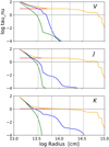 |
Fig. A.1 log optical depth vs log distance to stellar centre: green denote continuous opacities, blue line opacities, red dust opacities, and orange total opacity; vertical lines at 1, 2, 5, 10 stellar radii. Model is 2600/4.0/1.5 C7u6. SDDO and Max phase. |
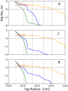 |
Fig. A.2 Log optical depth versus log distance to stellar centre: green continuous opacities, blue line opacities, red dust opacities, and orange total opacity; vertical lines at 1, 2, 5, 10 stellar radii. Model is 2600/4.0/1.5 C7u6. SPL and max phase. |
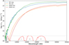 |
Fig. A.3 Spectra for the model 2600/4.0/1.5 C7u6 at a maximum and a minimum phase, as well as for the SPL and SDDO cases (see legend). |
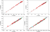 |
Fig. A.4 Median magnitudes versus mean magnitudes plotted for models in the SDDO grid. The different panels show the effects in the V, J, H, and K filters. The models are colour-coded according to their carbon excess (see Fig. 6). Offsets from the one-to-one line of 0.5 and 1.0 (in V), 0.2 and 0.5 (in J), and 0.1 and 0.2 (in H and K) are indicated by the grey lines. |
Appendix B Median versus mean magnitudes
If a light curve is asymmetric in time, for example with rather narrow minima and broader maxima, there can be a difference between the mean and the median magnitude. We also calculated the median for the light curves of the models in the SDDO grid. In Fig. A.4, we show the effects in the V, J, H, and K filters. We
note that the effect of replacing the mean by the median magnitude results in generally brighter magnitudes, but the effect is small, except for some of the highest carbon excess (C7) models.
Appendix C Model overview
A table with photometric and dynamic properties of the models in the present grid is found in electronic form at the CDS. The models are arranged by increasing effective temperature, luminosity, and stellar mass. For each such combination, the data are ordered by increasing carbon excess and piston velocity amplitude. In each line, after the model parameters we list the log g (surface gravity in cgs units). Then come dynamic quantities evaluated at the outer boundary: mass-loss rate (in solar masses per year), the wind velocity (km/s), the carbon condensation degree, and the dust-to-gas ratio. We note that all given values are temporal means (see Sect. 3). Then follow the photometric properties: the (full) amplitude of the bolometric magnitude, the mean V magnitude, the range of V magnitudes, the mean K magnitude and its range, and finally the colours (V–I), (V–K), (J–H), and (H–K).
The luminosities and stellar masses are given in solar units. The carbon excesses, log(C–0)+12, are given on the scale where log NH ≡ 12.00. The piston velocity amplitudes, ∆up, are given in km/s. All the photometric quantities are given in magnitudes. The first lines are shown below as an example.
Dynamic and photometric properties of the models in the present grid. The meaning and units for the different columns are described in Sect. C. The full table is available at the CDS.
The actual size distribution, n(agr)dagr, is not known during a simulation run, but can, in principle, be reconstructed afterwards.
www.astro.princeton.edu/~draine/scattering.html
The relation between the carbon excess, log(C–O) + 12, and the commonly used quantity C/O is given in Table 2. In contrast to other papers in the literature, we used the carbon excess to characterise the models, because this quantity directly translates into the amount of carbon available for the formation of carbon-bearing molecules (other than CO) and dust grains.
The P–L relation by Feast et al. (1989) is based on Miras in the LMC. In a diagram of K magnitudes versus period as, for example, in Ita et al. (2004), our models would largely overlap with the observed stars in sequence C. The stars belonging to this sequence are commonly believed to be fundamental mode pulsators (Wood et al. 1999).
All Tables
Relation between the carbon excess measure log(C–O) + 12 and the C/O ratio for the adopted chemical composition (Asplund et al. 2005), i.e. using an oxygen abundance of log(NO/NH)+12 = 8.66.
Dynamic and photometric properties of the models in the present grid. The meaning and units for the different columns are described in Sect. C. The full table is available at the CDS.
All Figures
|
Fig. 1 Efficiency factors as a function of grain size for an amC particle computed with full Mie theory (lines dashed red: absorption; dash-dotted blue: scattering; black: radiative pressure) and in the SPL approximation (absorption, plus signs). Top panel: values at a wavelength of 0.54 μm (V band). Bottom panel: values at a wavelength of 2.1 μm (K band; see text for details). While scattering is negligible in the SPL, it contributes significantly to the radiation pressure for particles with sizes that are comparable to the wavelength. |
| In the text | |
|
Fig. 2 Dynamic behaviour of models these are also referred to as wind-maps. In an HR-type display, the models are colour-coded as red for wind, blue for no wind, and green for episodic behaviour. The upper four panels show the SDDO case and the lower four show the grid with the SPL approximation. The four sub-panels for each grid show models of different stellar masses indicated in the top left corner. For each given combination of temperature and luminosity, the different carbon excesses and piston amplitudes are arranged as shown in the bottom legend. |
| In the text | |
|
Fig. 3 Comparison of different properties of SDDO versus SPL grids. The quantities plotted are mass-loss rates (upper left), outflow speeds (upper right), condensation degrees (lower left) and dust grain radii (lower right). The different carbon excesses are shown in colour: log(C-O) = 8.2 in green, 8.5 in blue, and 8.8 in red. Circles denote wind models and triangles denote episodic models. |
| In the text | |
|
Fig. 4 Gas density at outer boundary as a function of time for selected models with a stellar mass of 0.75 M⊙. The left column displays the SDDO values, the right one the SPL values. Stellar parameters, Teff, log L, carbon excess class and piston amplitude, are given in the SPL panels. The densities are given in cgs units: Teff in K, log L in L⊙, and piston amplitudes in km s−1. We use a fixed range in gas density in all panels. |
| In the text | |
|
Fig. 5 Gas density at the outer boundary as a function of time for 1.5 M⊙ models (see Fig. 4 for details). |
| In the text | |
|
Fig. 6 Mean K magnitude for models in the entire grid computed without using the dust opacity in the a posteriori radiative transfer (COMA). The values for the SDDO cases versus the SPL ones are plotted. |
| In the text | |
|
Fig. 7 Mean V, J, H, and K magnitude for models in the entire grid. The values for the SDDO cases versus the SPL ones are plotted. Colours and symbols are explained in Fig. 6. |
| In the text | |
|
Fig. 8 Mean V magnitude for wind models in the SDDO versus SPL cases. In the left panel, the points are colour-coded according to Q(SDDO)/Q(SPL) and evaluated at appropriate grain radii. In the right panel, the colour is given by the ratio of the mean condensation degree in the SDDO and the SPL cases. |
| In the text | |
|
Fig. 9 Photometrie variations of the models shown in the top row of Fig. 5. The (J–H) versus (H–K) diagram (top left) and the light curves of the V (top right), J (bottom left), and K (bottom right) magnitudes for three periods in several epochs. The SDDO values are plotted in orange-red hues, and the SPL values are plotted in blue-ones. The model has the parameters Teff = 2600 K, log L = 4.0 L⊙, mass 1.5 M⊙, log(C–O) = 8.5, and a piston amplitude of 4 km s−1. |
| In the text | |
|
Fig. 10 As Fig. 9, but for the models with log(C–O) = 8.8 and piston amplitude of 6 km s−1 (bottom row in Fig. 5). |
| In the text | |
|
Fig. 11 Mean range in K magnitudes for models in the entire grid. The SDDO values are plotted versus the SPL ones. Colours and symbols are explained in Fig. 6. |
| In the text | |
|
Fig. 12 Mean amplitude in V magnitudes (left) and their range (right) for models in the entire grid. The SDDO values are plotted versus the SPL ones. The models are colour-coded according to their carbon excess (see Fig. 6). In the right panel, the area of the left panel is outlined. |
| In the text | |
|
Fig. 13 Mass-loss rates versus outflow speeds for wind models in the grid for the SDDO case. The different colours denote the carbon excess. Colours and symbols are explained in Fig. 6. Observational data from Schöier & Olofsson (2001) and Ramstedt & Olofsson (2014) are plotted as grey symbols. |
| In the text | |
|
Fig. 14 Mean (J–H) colour versus mean (H–K) colour for models in the entire grid. Models using SPL are plotted in grey tones, and those with SDDO are coloured according to carbon excess (see Fig. 6). Observed carbon stars from Whitelock et al. (2006) are also plotted: orange symbols for Miras and cyan for non-Mira stars. The grey box centered at (0.5, 1.0) outlines the area in Fig. 15. |
| In the text | |
|
Fig. 15 (J–H) versus (H–K) for hydrostatic dust-free carbon star models from the COMARCS grid presented in Aringer et al. (2016, 2019, green squares). Two C/O ratios are shown: 1.4 and 2.0. The results are compared to a similar grid computed with updated opacities for molecular and atomic transitions (red circles). The large shift between the two sets of models is due to changes of the absorption caused by C2 and C2H2. In addition, observed values of carbon stars are included (crosses); they cover objects with solar and subsolar metallicities (see text). |
| In the text | |
|
Fig. 16 MK values versus mean (J–K)0 colour for SDDO models in the entire grid. Colours and symbols are explained in Fig. 6. Observed carbon Mira stars from Whitelock et al. (2006) are plotted as orange symbols, and those from Menzies et al. (2006) are plotted as green symbols. |
| In the text | |
|
Fig. 17 MJ values versus mean (J–K)0 colour for the SDDO models in the entire grid. Colours and symbols are explained in Fig. 6. The value of MJ = −6.2 is marked, as well as (J–K)0 = 1.4 and 2.0. |
| In the text | |
|
Fig. 18 Mass-loss rate versus mean (J–K)0 colour for the SDDO wind models in the grid. The colours denote the carbon excess (see Fig. 6), the circles with different grey hues are the SPL models. Observed carbon Mira stars from Whitelock et al. (2006) are plotted as orange symbols, while observations from Schöier & Olofsson (2001) and Ramstedt & Olofsson (2014) are plotted as blue symbols (or green if the source is also present as an orange symbol from Whitelock et al. 2006). |
| In the text | |
|
Fig. 19 Mean gas-to-dust ratio for the wind models in the grid plotted against the mean (J–K) colour (top panel) and against the mean mass-loss rate (lower panel). The models are colour-coded for the carbon excess (see Fig. 6). For models computed with the SPL, we use grey symbols. |
| In the text | |
|
Fig. 20 Mean dust-mass-loss rate versus mean (J–K)0 colour for the wind models in the grid. The observed dust-mass-loss rates (plotted as orange symbols) were derived from total mass-loss rates in Whitelock et al. (2006) using a gas-to-dust ratio of 220. |
| In the text | |
|
Fig. A.1 log optical depth vs log distance to stellar centre: green denote continuous opacities, blue line opacities, red dust opacities, and orange total opacity; vertical lines at 1, 2, 5, 10 stellar radii. Model is 2600/4.0/1.5 C7u6. SDDO and Max phase. |
| In the text | |
|
Fig. A.2 Log optical depth versus log distance to stellar centre: green continuous opacities, blue line opacities, red dust opacities, and orange total opacity; vertical lines at 1, 2, 5, 10 stellar radii. Model is 2600/4.0/1.5 C7u6. SPL and max phase. |
| In the text | |
|
Fig. A.3 Spectra for the model 2600/4.0/1.5 C7u6 at a maximum and a minimum phase, as well as for the SPL and SDDO cases (see legend). |
| In the text | |
|
Fig. A.4 Median magnitudes versus mean magnitudes plotted for models in the SDDO grid. The different panels show the effects in the V, J, H, and K filters. The models are colour-coded according to their carbon excess (see Fig. 6). Offsets from the one-to-one line of 0.5 and 1.0 (in V), 0.2 and 0.5 (in J), and 0.1 and 0.2 (in H and K) are indicated by the grey lines. |
| In the text | |
Current usage metrics show cumulative count of Article Views (full-text article views including HTML views, PDF and ePub downloads, according to the available data) and Abstracts Views on Vision4Press platform.
Data correspond to usage on the plateform after 2015. The current usage metrics is available 48-96 hours after online publication and is updated daily on week days.
Initial download of the metrics may take a while.