| Issue |
A&A
Volume 672, April 2023
|
|
|---|---|---|
| Article Number | A119 | |
| Number of page(s) | 30 | |
| Section | Stellar structure and evolution | |
| DOI | https://doi.org/10.1051/0004-6361/202245712 | |
| Published online | 10 April 2023 | |
The Araucaria project: High-precision orbital parallaxes and masses of binary stars
I. VLTI/GRAVITY observations of ten double-lined spectroscopic binaries⋆
1
Universidad de Concepción, Departamento de Astronomía, Casilla 160-C, Concepción, Chile
e-mail: This email address is being protected from spambots. You need JavaScript enabled to view it.
2
French-Chilean Laboratory for Astronomy, IRL 3386, CNRS, Casilla 36-D, Santiago, Chile
3
European Southern Observatory, Karl-Schwarzschild-Str. 2, 85748 Garching, Germany
4
LESIA, Observatoire de Paris, CNRS UMR 8109, UPMC, Université Paris-Diderot, 5 place Jules Janssen, 92195 Meudon, France
5
Centrum Astronomiczne im. Mikołaja Kopernika, Polish Academy of Sciences, Rabiańska 8, 87-100 Toruń, Poland
6
Centrum Astronomiczne im. Mikołaja Kopernika, Polish Academy of Sciences, Bartycka 18, 00-716 Warsaw, Poland
Received:
17
December
2022
Accepted:
8
February
2023
Abstract
Aims. We aim to measure very precise and accurate model-independent masses and distances of detached binary stars. Precise masses at the < 1% level are necessary to test and calibrate stellar interior and evolution models, while precise and independent orbital parallaxes are essential to check for the next Gaia data releases.
Methods. We combined RV measurements with interferometric observations to determine orbital and physical parameters of ten double-lined spectroscopic systems. We report new relative astrometry from VLTI/GRAVITY and, for some systems, new VLT/UVES spectra to determine the radial velocities of each component.
Results. We measured the distance of ten binary systems and the mass of their components with a precision as high as 0.03% (average level 0.2%). They are combined with other stellar parameters (effective temperatures, radii, flux ratios, etc.) to fit stellar isochrones and determine their evolution stage and age. We also compared our orbital parallaxes with Gaia and showed that half of the stars are beyond 1σ with our orbital parallaxes; although, their RUWE is below the frequently used cutoff of 1.4 for reliable Gaia astrometry. By fitting the telluric features in the GRAVITY spectra, we also estimated the accuracy of the wavelength calibration to be ∼0.02% in high and medium spectral resolution modes.
Conclusions. We demonstrate that combining spectroscopic and interferometric observations of binary stars provides extremely precise and accurate dynamical masses and orbital parallaxes. As they are detached binaries, they can be used as benchmark stars to calibrate stellar evolution models and test the Gaia parallaxes.
Key words: binaries: general / binaries: spectroscopic / techniques: high angular resolution / astrometry / binaries: close / techniques: radial velocities
Based on observations made with ESO telescopes at Paranal and La Silla observatory under programme IDs 0104.D-0191(A), 105.207C.001, 106.210E.001, 106.210E.002, 108.221X.001, 108.221X.003, 109.22XY.001, 109.22XY.002, 109.22XY.003, and 110.23QY.001.
© The Authors 2023
 Open Access article, published by EDP Sciences, under the terms of the Creative Commons Attribution License (https://creativecommons.org/licenses/by/4.0), which permits unrestricted use, distribution, and reproduction in any medium, provided the original work is properly cited.
This article is published in open access under the Subscribe to Open model. This email address is being protected from spambots. You need JavaScript enabled to view it. to support open access publication.
1. Introduction
Stars in detached binary systems are the only tool enabling direct and precise distance and mass measurements. When the spectral lines of both components can be detected, the radial velocity (RV) of the orbital motion around the centre of mass of the two stars can be measured, providing the spectroscopic orbit of the system. However, this only provides the spectroscopic mass function, which is a combination of the stellar masses. With the apparent orbit from astrometry, we can measure the orbital inclination and obtain the individual masses of the system. In addition, spectroscopy provides the projected linear semi-major axis while astrometry gives its angular size, which directly provides the distance to the system. This is the only geometric and model-independent way of measuring masses and distances of stars (see e.g. McAlister 1976; Pourbaix et al. 2004; Torres 2004; Docobo & Andrade 2013; Torres et al. 2015; Gallenne et al. 2016).
The main source providing precise stellar parameters is eclipsing binary (EB) systems, which combines RVs with photometric measurements during the eclipses (see e.g. Andersen & Vaz 1984; Milone et al. 1992; Pietrzyński et al. 2009, 2013, 2019; Kirkby-Kent et al. 2016; Graczyk et al. 2020). Although a precision level of 1 − 3% is routinely achieved, it is still subject to some modelling of the light curves, such as for the limb darkening, oblateness, or stellar spots. To determine the distance, a surface brightness colour relation is usually used to estimate the angular diameter of the stars, which is then combined with the linear value measured from the eclipses. EBs are a powerful tool and already provide precise masses and distances; however, this still depends on some modelling and relations that need to be well calibrated.
Combining astrometry with RV is the best way to measure the basic stellar properties using a minimum of theoretical assumptions. An astrometric orbit can be measured using different observing techniques. The most commonly used one is direct imaging which allows one to resolve the components to then monitor their relative position with time to cover the orbit. Direct imaging is sensitive to wide binaries, and therefore to systems with very long orbital periods making observations impractical. If the faintest (secondary) component is not seen as a separate star, we can sometimes infer its presence from the gravitational influence on the main visible (primary) component. The detection of the primary wobble requires long-term observations and a good precision on the measured positions and proper motions, in addition to needing the secondary companion to be massive enough to produce a detectable effect. Thousands of binaries were detected this way by the HIPPARCOS telescope (Perryman et al. 1997; Lindegren et al. 1997) and in the Gaia data release 3 (DR3; Halbwachs et al. 2023; Gaia Collaboration 2016). Many more will be discovered with the improved precision of Gaia (see e.g. Kervella et al. 2019a,b). Speckle imaging is also a well-established technique for obtaining diffraction-limited images and to monitor orbits of binary stars, providing an overlap with long baseline interferometry (see e.g. Horch et al. 2020; Tokovinin & Horch 2016). Interferometric observing techniques allow for astrometric measurements of binary stars by probing a different spatial scale, well below the diffraction limit of a single-dish telescope. Very high spatial resolution can be explored with optical long-baseline interferometry (LBI, see e.g. Lawson 2000), down to a few milli-arcsecond (mas). LBI enables the astrometric detection of close-in binaries (< 20 mas, see e.g. Hummel et al. 1994, 2001; Zhao et al. 2007; Konacki et al. 2010), with such a small angular resolution so that more complex systems can be observed, such as interacting binaries (Zhao et al. 2008) or an eclipsing system with one component enshrouded in an accretion disk (Kloppenborg et al. 2010). LBI has now proven its efficiency in terms of angular resolution and accuracy for close-in binary stars (see e.g. Baron et al. 2012; Le Bouquin et al. 2013; Gallenne et al. 2013, 2014, 2015; Gallenne et al. 2016, 2018a, 2019; Pribulla et al. 2018; Gardner et al. 2018, 2021; Lester et al. 2020), and it can now reach a few μas in astrometric precision.
In this series of papers, we use LBI to observe simple double-lined spectroscopic binary (SB2) systems, that is non-interacting binary systems. This way, the systems are free of any modelling assumptions, and our main objective is to provide very precise and accurate mass and distance measurements. We have shown in our previous studies (Gallenne et al. 2016, 2019) that mass accuracies as high as 0.05% can be achieved combining RVs and LBI. The mass is a fundamental parameter in order to understand the structure and evolution of stars, and very precise measurements are necessary to check the consistency with theoretical models and to tighten the constraints. For now, stellar parameters (e.g. the effective temperature and radius) predicted from different stellar evolution codes can lead to discrepancies with the empirical values, and therefore provide a large range of possible ages for a given system (see e.g. Torres et al. 2010; Gallenne et al. 2016). Stellar interior models differ in various ways, for instance in input physics, initial chemical compositions, their treatment of convective-core overshooting, and using rotational mixing or the mixing length parameter (Marigo et al. 2017; Bressan et al. 2012; Dotter et al. 2008; Pietrinferni et al. 2004). With high-precision measurements, evolutionary models can be tightly constrained and provide a better understanding of stellar interior physics, enabling the calibration of the physics within evolutionary models. Recent work has shown that a significant improvement in precision on the stellar mass ≪1% is necessary to obtain reliable determinations of the stellar interior model parameters (overshooting, initial helium abundance, etc., see e.g. Valle et al. 2017; Claret & Torres 2018; Higl et al. 2018).
Our previous works combining SB2 systems with LBI (Gallenne et al. 2016, 2019) also demonstrate that very precise and accurate distances can be measured, down to 0.35%. The knowledge of distances is important in many fields of astrophysics. Gaia is revolutionising the field with precise parallax measurements, but it still suffers from some calibration or systematic biases (Lindegren et al. 2021a). Independent, precise, and accurate geometric distance measurements from binary systems provide a unique benchmark on which to test Gaia parallaxes (see e.g. Southworth & Bowman 2022; Graczyk et al. 2021; Gallenne et al. 2019).
In this paper, we report new spectroscopic and interferometric observations of ten binary systems, including three eclipsing ones. In Sect. 2, we describe the observations and the data reduction methods. The main improvement since our previous works is the use of the GRAVITY beam combiner of the Very Large Telescope Interferometer (VLTI) to perform relative astrometry. We previously used the VLTI/PIONIER instrument (Precision Integrated-Optics Near-infrared Imaging ExpeRiment, Le Bouquin et al. 2011), which limited the accuracy of any dimensional measurement to 0.35% (Gallenne et al. 2018b) due to the internal calibration of the instrument wavelength scale. Thanks to a dedicated internal reference laser source, the GRAVITY instrument can provide a much better accuracy, down to 0.02% with high spectral resolution and 0.05% in medium resolution (GRAVITY Collaboration, priv. comm.), which we verified in Sect. 2.3 by fitting telluric lines. We present in Sect. 3 our fitting formalism and the results obtained for each system in Sect. 4. We conclude in Sect. 7.
2. Observations and data reduction
2.1. Spectroscopic data and radial velocities
We report new observations with the UV Echelle Spectrograph (UVES; Dekker et al. 2000) mounted on the ESO Very Large Telescope (VLT). We simultaneously used the UVES blue and red arms of the instrument, centred on 390 nm and 584 nm with a slit width of 0.4″ and 0.3″, respectively. This provides a resolving power of ∼80 000 and ∼110 000 in the blue and red arm, respectively, covering the spectral range 0.3 − 0.7 μm. For each observation, a thorium-argon lamp exposure was taken immediately after each science spectrum in order to achieve the best calibration of a few m s−1 in precision.
As our stars are bright, each observation has only one exposure of a few seconds. This programme was executed using the ‘filler’-type observations, and the stars were observed in non-optimal conditions in terms of seeing, cloud coverage, etc. Despite these limitations, we have spectra of really good quality with a high signal-to-noise ratio (S/N), ranging from ∼30 to ∼500. Raw data were reduced using the UVES pipeline v6.1.6 within the EsoReflex environment (Freudling et al. 2013).
To extract the RVs, we used the broadening function (BF) formalism (Rucinski 1999) implemented in the RaveSpan software1 (Pilecki et al. 2017; see also e.g. Pilecki et al. 2018, 2013; Gallenne et al. 2016; Graczyk et al. 2015). We used templates from the synthetic library of LTE spectra of Coelho et al. (2005) in the range 3760 − 4520 Å, 4625 − 5600 Å, and 5675 − 6645 Å (corresponding to the BLUE, REDL, and REDU UVES spectra). For some stars, the S/N was low in the blue part, so we only kept the red part. The templates were chosen to match the atmospheric properties of the hottest star in the systems. They were taken from the literature and are listed in Table 1. The errors of RVs were measured from the broadening function profiles. Our measured UVES RVs are listed in Table C.1.
Stellar atmospheric parameters of the hottest component used for the spectral templates to estimate the radial velocities.
We also gathered precise RVs from the literature. In some cases, fitting both the literature’s and our RVs degraded the final mass and distance accuracy, either because those from the literature were not precise enough or they had a large scatter, so we only used our RVs whenever necessary. In other cases, we did not have UVES observations and only RVs from the literature were used. Additional observations for some targets were also executed as backup targets by our team with the High-Accuracy Radial-velocity Planet Searcher (HARPS) spectrograph mounted on the 3.6 m telescope at La Silla observatory (Pepe et al. 2002). The HARPS spectrograph provides a high spectral resolution of R ∼ 115 000 in the wavelength range 3800 − 6900 and allows for precise RV measurements. The data were reduced by the instrument data reduction software. Our spectroscopic dataset was supplemented with public HARPS-reduced spectra downloaded from the ESO archive2 and public SOPHIE-reduced spectra downloaded from the dedicated database3. SOPHIE (Spectrographe pour l’Observation des Phénomènes des Intérieurs stellaires et des Exoplanètes, Bouchy & Sophie Team 2006) is also a visible echelle spectrograph providing a resolution R ∼ 40 000 in high-efficiency mode. All RVs were estimated the same way as described previously. A summary of the RVs used is listed in Table 2.
References for the radial velocity we used in this work.
2.2. Interferometric data
Observations were performed with the four-telescope combiner GRAVITY (Eisenhauer et al. 2011), the second-generation instrument of the VLTI (Haguenauer et al. 2010). As our stars are bright, we used the auxiliary telescopes (ATs) of the VLTI and the single-field mode of the instrument, meaning that the incoming light is split between the fringe tracker (FT) and the science combiner (SC) with a 50%–50% beam splitter. GRAVITY simultaneously combines the light coming from four telescopes in the K band and delivers spectrally dispersed interference fringes for three spectral resolution for the science channel (R ∼ 22, 500, and 4000), while the FT only operates at low spectral resolution (R ∼ 22). The FT allows for a longer integration time on the SC thanks to a real-time analysis of the fringe position to correct for the atmospheric and instrumental piston. The final main observables are the visibilities (|V|), squared visibilities (V2), and the closure phases (CPs) (the bispectrum amplitude T3amp has not been validated in commissioning yet). In some cases, when a spectral feature is expected (e.g. Hα emission line for a Be star), differential visibilities and phases are also useful in the spectral model, but not particularly needed to study astrometric orbits.
We observed ten double-lined spectroscopic binaries from 2019 to 2021 in medium and high spectral resolution mode with the medium and large quadruplets, providing baselines up to 140 m. To monitor the instrumental and atmospheric contributions, we used the standard observational procedure, which consists of observing a reference star before or after the science target. The calibrators, listed in Table B.1 and detailed in Table D.1, were selected using the SearchCal4 software (Bonneau et al. 2006, 2011; Chelli et al. 2016) provided by the Jean-Marie Mariotti Center (JMMC).
The data were reduced with the GRAVITY data reduction pipeline described in Lapeyrere et al. (2014). The main procedure is to compute squared visibilities and triple products for each baseline and spectral channel, and to correct for photon and readout noises. In Fig. 1, we present an example of the observables for one observation of AK For. The binary nature of the system is clearly detected.
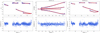 |
Fig. 1. Squared visibility, closure phase, and visibility measurements from the science combiner for AK For observed on 2021 November 8. The data are in blue, while the red dots represent the fitted binary model for this epoch. The residuals (in number of sigma) are also shown in the bottom panels. |
For each epoch, we proceeded to a grid search to find the global minimum and the location of the companions. For this, we used the interferometric tool CANDID5 (Gallenne et al. 2015) to search for the companion using all available observables. CANDID allows for a systematic search for point-source companions performing an N × N grid of fit, whose minimum required grid resolution is estimated a posteriori. The tool delivers the binary parameters, that is, the flux ratio f and the relative astrometric separation (Δα, Δδ). CANDID can also fit the angular diameter of both components; however, in our case, we kept them fixed for most systems (nine out of ten) during the fitting process as the VLTI baselines do not allow for reliable measurements of small diameters. For each epoch, CANDID found the global best-fit separation vector. The final astrometric positions for all epochs of all systems are listed in Table B.1. We estimated the uncertainties from the bootstrapping technique (with replacement) and 10 000 bootstrap samples (also included in the CANDID tool). For the flux ratio, we considered the median value and the maximum value between the 16th and 84th percentiles from the distributions as uncertainty. For the astrometry, the 1σ error region of each position (Δα, Δδ) is defined with an error ellipse parametrised with the semi-major axis σmaj, the semi-minor axis σmin, and the position angle σPA measured from north to east.
To reach the highest astrometric precision, we only used data from the science combiner because of the systematic uncertainty from the precision of the GRAVITY wavelength calibration. The SC provides a calibration at a sub-percent level, but the FT has a lower precision due to its low spectral resolution and it would limit our final precision on the distance of the binary systems.
As mentioned previously, the primary angular diameters of nine systems are too small to be spatially resolved by the VLTI. We therefore kept them fixed during the grid search with the values given in Table 3. We note that angular diameters do not significantly affect the measured astrometry (the flux ratio is the most affected). In some cases where there is no binary signature in the CPs, the flux ratio is poorly constrained; we therefore fixed it to the average value estimated from the epoch with strong binary signature in all observables. Gallenne et al. (2019) investigated the effect of fitting or fixing the flux ratio in deriving astrometric positions for very nearby components (i.e. < λ/2B) and show that the agreement in fixing the flux ratio or not stays within 1σ. The astrometric measurements are reported in Table B.1.
Angular diameters taken from the literature.
2.3. Astrometric accuracy of interferometric data
The accuracy of the interferometric astrometry is dominated by the uncertainties in the knowledge of the spatial frequency B/λ, where B is the projected baseline and λ the wavelength of observations. The VLTI baselines are determined by observing stars all over the sky and recording their absolute fringe position using the delay line laser metrology. This process leads to a baseline scaled to the calibrated metrology laser, which is typically known to 0.02 parts per million.
The wavelength of the instrument is a much larger source of potential inaccuracy of the spatial frequency scaling. GRAVITY is equipped with a spectrograph calibrated using a dedicated Argon lamp. Because GRAVITY is not a conventional spectrograph, and since spectral data are transformed and resampled (Lapeyrere et al. 2014), the resulting spectral accuracy is expected to be of the order of the spectral resolution: in high resolution mode (R ∼ 4000), the spectral accuracy is expected to be ∼0.55 nm (0.025%), whereas in medium resolution (R ∼ 500), it is expected to be ∼4.4 nm (0.2%). One can verify the final accuracy of the spectral calibration by fitting the telluric features in the GRAVITY spectra. We did this using PMOIRED6 (Mérand 2022) using a synthetic interpolated grid of telluric spectra computed with MOLECFIT (Smette et al. 2015). For the AK For dataset, we find an average wavelength bias per epoch ranging from ∼ − 0.006% to ∼ + 0.019% in both medium and high spectral resolution mode. The spectral calibration is displayed in Fig. A.1. This confirms that taking the spectral resolution for the accuracy of the spectral calibration is a reasonable choice in high resolution, whereas it is better than expected in medium resolution. We chose to add a 0.02% systematic error to each astrometric measurement for observations for both spectral resolutions.
We also investigated the effect of static optical aberrations on the visibility measurements across the field of view (FoV). This was first assessed with GRAVITY in low resolution mode for the Galactic Centre by GRAVITY Collaboration (2021), who developed a full analytical model describing the effect of these aberrations on the measurement of complex visibilities. Their analysis has shown that small optical imperfections induce field-dependent phase errors, which can affect the measured binary separation. In addition, misalignments of the injection fibres with respect to the centre of the FoV can also introduce phase errors. They used the GRAVITY calibration units (Blind et al. 2014) to measure the static aberrations of the science channel and to construct a complex aberration map, which is then used in fitting a binary model to complex visibilities. They present a binary test case with a 200 mas separation observed with the ATs, and show that accurate astrometry mostly depends on a consistent treatment of the pupil-plane distortions rather than a precise fibre alignment. They also demonstrate that in the specific case of the S2 orbit around the Galactic Centre, phase aberrations introduced a shift up to 0.5 mas on the separation, which is not negligible. In this paper, our binaries have angular separations substantially smaller than the binary cases reported by GRAVITY Collaboration (2021). To quantify the effect of static aberrations on smaller binary separations, we performed our own test using the public script provided by the GRAVITY team to create aberration maps7 and extract the amplitude, phase error, and intensity at the given position in the fibre. Our tests consisted in comparing different binary star models (i.e. various separations and flux ratios) with and without static aberrations in order to assess an additional systematic uncertainty. We created binary models of two unresolved stars with flux ratios of 5%, 10%, 30%, 50%, and 80%; separations of 2, 5, 10, 15, 20, 30, and 50 mas; and projection angles of 0, 45, 90, 135, 180, 225, 270, and 315° (we set the typical error of 2% on the visibilities and 0.5° for the closure phases). In addition, for each position (Δα, Δδ), we added a random offset in the range [ − 0.3, 0.3] mas at each telescope (from a uniform distribution) to take possible fibre misalignments into account. We chose this range because it corresponds to about twice the mean value of all offsets of our entire dataset8. We then fitted all models around the expected astrometric positions with the flux ratios kept fixed and compared the fitted positions with the expected ones. We report the standard deviation of the residual in Δα and Δδ of all fits in Table 4 (i.e. the standard deviation of the fitted minus expected values). We see that fibre misalignments slightly contribute to the error and optical aberrations have more of an impact on low flux ratios, and they decrease with increasing flux ratios. For our binary systems, we have flux ratios > 8%, and therefore the additional errors due to optical aberrations and fibre misalignments would be < 50 μas. We quadratically added this error to our astrometric measurements according to the flux ratio of a given system, that is 50, 20, 12, and 8 μas for f ∼ 10, 30, 50, and 80%, respectively.
Standard deviation of the residuals between the fitted and expected positions of our synthetic companions.
3. Orbit fitting
We used the same formalism as in Gallenne et al. (2019). We simultaneously fitted the RVs and astrometric positions using a Markov chain Monte Carlo (MCMC) routine9. The log-likelihood function is defined with the following:
Radial-velocity measurements are related to the orbital elements with
in which Vi and σVi denote the measured RVs and uncertainties for the component i. In addition, (V1m, V2m) are the Keplerian velocity models of both components, defined by (Heintz 1978)
![Mathematical equation: $$ \begin{aligned}&V_{\rm 1m} = \gamma + K_1\,[\cos (\omega + \nu ) + e\cos {\omega }], \\&V_{\rm 2m} = \gamma - K_2\,[\cos (\omega + \nu ) + e\cos {\omega }], \\&\tan \dfrac{\nu }{2} = \sqrt{\dfrac{1 + e}{1 - e}} \tan \dfrac{E}{2}, \\&E - e \sin E = \dfrac{2\pi (t - T_{\rm p})}{P_{\rm orb}}, \end{aligned} $$](/articles/aa/full_html/2023/04/aa45712-22/aa45712-22-eq3.gif)
where γ is the systemic velocity, e the eccentricity, ω the argument of periastron, ν the true anomaly, E the eccentric anomaly, t the observing date, Porb the orbital period, and Tp the time of periastron passage. The parameters K1 and K2 are the RV amplitude of both stars.
The astrometric measurements are fitted as
![Mathematical equation: $$ \begin{aligned} \chi ^2_{\rm ast}&= \chi ^2_{\rm a} + \chi ^2_{\rm b}, \\ \chi ^2_{\rm a}&= \sum \frac{[ (\Delta \alpha - \Delta \alpha _{\rm m}) \sin \sigma _{\rm PA} + (\Delta \delta - \Delta \delta _{\rm m}) \cos \sigma _{\rm PA} ]^2}{\sigma ^2_{\rm maj}}, \\ \chi ^2_{\rm b}&= \sum \frac{[ -(\Delta \alpha - \Delta \alpha _{\rm m}) \cos \sigma _{\rm PA} + (\Delta \delta - \Delta \delta _{\rm m}) \sin \sigma _{\rm PA} ]^2}{\sigma ^2_{\rm min}}, \end{aligned} $$](/articles/aa/full_html/2023/04/aa45712-22/aa45712-22-eq4.gif)
in which (Δα, Δδ, σPA, σmaj, σmin) denote the relative astrometric measurements with the corresponding error ellipses, and (Δαm, Δδm) the astrometric model can be defined with
![Mathematical equation: $$ \begin{aligned}&\Delta \alpha _{\rm m} = r \,[ \sin \Omega \cos (\omega + \nu ) + \cos i \cos \Omega \sin (\omega + \nu ) ], \\&\Delta \delta _{\rm m} = r \,[ \cos \Omega \cos (\omega + \nu ) - \cos i \sin \Omega \sin (\omega + \nu ) ], \\&r = \dfrac{a (1 - e^2)}{1 + e\cos \nu }, \end{aligned} $$](/articles/aa/full_html/2023/04/aa45712-22/aa45712-22-eq5.gif)
where Ω is the longitude of ascending node, i the orbital inclination, and a the angular semi-major axis.
As a starting point for our 100 MCMC walkers, we performed a least squares fit using orbital values from the literature as first guesses. We then ran 100 initialisation steps to thoroughly explore the parameter space and get settled into a stationary distribution. The prior distributions used are uniform for all parameters and are listed in Table 5. For all cases, the chain converged before 50 steps. Finally, we used the last position of the walkers to generate our full production run of 1000 steps, discarding the initial 50 steps. All the orbital elements, that is Porb, Tp, e, ω, Ω, K1, K2, γ, a, and i, were estimated from the distribution considering the median value and the maximum value between the 16th and 84th percentiles as uncertainty (although the distributions were roughly symmetrical).
Uniform prior distributions used.
The distributions of the mass of both components and the distance were derived from the MCMC distributions with (Torres et al. 2010)

where the masses are expressed in solar units, the distance in parsec, K1 and K2 in km s−1, P in days, and a in arcsecond. The parameter aAU is the linear semi-major axis expressed in astronomical units (the constant value of Torres et al. (2010) is expressed in solar radii, and was converted using the astronomical constants R⊙ = 695.658 ± 0.140 × 10⁶ m from Haberreiter et al. 2008 and AU = 149 597 870 700 ± 3 m from Pitjeva & Standish 2009). As was previously done, we then took the median value and the maximum value between the 16th and 84th percentiles as uncertainty. The fitting results are presented in the next section for all systems.
4. Results for individual systems
4.1. AK Fornacis
This is a low-mass eclipsing binary system composed of two similar main-sequence stars in a 3.98 d orbit. Hełminiak et al. (2014) studied this system using both RVs and photometry during eclipses and derived very precise stellar parameters. We used the RVs they reported (from the CORALIE and FEROS spectrographs) and we complemented the dataset with HARPS data. A zero-point offset between our RVs and those from Hełminiak et al. (2014) were determined by fitting each dataset independently, and taking the difference in the systemic velocities. We found an offset of +261 m s−1 which we added to the HARPS RVs. Our final parameters measured from our combined astrometric and RVs’ orbital fit are listed in Table 6, and the orbit is displayed in Fig. 2. We reached a rms of the astrometric orbit of 11 μas.
Best-fit orbital elements and parameters for our binary systems.
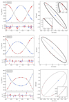 |
Fig. 2. From top to bottom: combined fit of AK For, HD 9312, and HD 41255. Left: radial velocities of the primary (blue) and the secondary (red) star. Right: GRAVITY astrometric orbit. The shaded grey area represents the 1σ orbit. |
Our measured masses have a precision ≤0.12%. They are in excellent agreement with the values derived by Hełminiak et al. (2014) at < 1σ, demonstrating that our measurements are both precise and accurate. We measured a distance to the system with an accuracy level of 0.17%, and in agreement at 0.7σ with the last Gaia data release (here and in the following, we applied a zero-point offset following the correction from Lindegren et al. 2021a). We also measured an average flux ratio fK = 71.7 ± 1.6% between the two components.
4.2. HD 9312
This SB2 system has two similar stars orbiting each other in a 36.5 d orbit. It was mainly studied using spectroscopy (see e.g. Katoh et al. 2021; Kiefer et al. 2018; Halbwachs et al. 2014), and no individual mass has been measured, but a mass ratio was derived to be q = 0.7624 ± 0.0015 from the cross-correlation function (CCF) of several spectra (Halbwachs et al. 2014). The SB2 orbit was only published recently by Kiefer et al. (2018). Wang et al. (2015) used an iterative method to determine self-consistent orbital solutions via a combined fit of the SB1 orbit and the HIPPARCOS Intermediate Astrometric Data, but their estimated mass ratio of 0.88 is larger than the one estimated by Halbwachs et al. (2014), although with a large uncertainty of ∼45%. Combining their fitted stellar parameters with evolutionary tracks, they show that the primary is on the subgiant giant branch while the secondary is on the main sequence.
Our combined fit with astrometry provides measured masses with a precision level of 0.3%. It is displayed in Fig. 2. The rms of the astrometric orbit is ∼50 μas. We corrected for a RV offset between our UVES RVs and Kiefer et al. (2018) of +0.304 km s−1. Our mass ratio is in very good agreement with the value derived by Halbwachs et al. (2014) at the < 0.1σ level. The spectroscopic orbital parameters estimated by Wang et al. (2015) are in agreement with our values, but their inclination is not consistent and it is ∼3σ smaller. The other astrometric orbital parameters, a and Ω, are also quite different, with an ∼1.5 mas difference for the semi-major axis. Their derived masses have a relative uncertainty of ∼30%, meaning that they are in agreement within 1σ with our measurements. The method applied by Wang et al. (2015) is not a direct measurement; it needs evolutionary models to estimate the primary mass and a mass luminosity relation for the secondary mass. This may explain the low precision on the masses.
We measured the distance to the system with a precision of 0.6% and this is in agreement with the Gaia measurement at ∼1.8σ. Our interferometric observations also provide a K-band flux ratio of 7.84 ± 0.49%.
4.3. HD 41255
The spectroscopic binary nature was only recently discovered by the Geneva-Copenhagen survey of the Solar neighbourhood (GCS; Holmberg et al. 2009), but no orbital parameters were determined. The double-line nature was detected by Gorynya & Tokovinin (2014) and they estimate a preliminary orbital period of 163 d and a mass ratio q = 0.98. The system is composed of two similar stars whose primary is a F8/G0V star. The spectroscopic orbital parameters were later determined by Gorynya & Tokovinin (2018) with an updated period of 148.3 d. They estimate a semi-major axis of 11 mas and predict an orbital inclination around 53°, which are very close to our measured values listed in Table 6.
We obtained a very precise orbit, as we can see in Fig. 2, which enabled us to measure the mass of both components at a 0.21% precision level. The stars have an equal mass with a ratio q = 1.008 ± 0.003, and they are solar-type stars. This is also consistent with the average K-band flux ratio fH = 95.9 ± 1.0% we determined from GRAVITY. We also measured the distance to the system at a 0.08% precision that is at 2.1σ to the Gaia estimate. We reached an unprecedented astrometric orbit rms of ≤11 μas.
4.4. HD 70937
This is a 28 d SB2 binary whose full spectroscopic orbital elements have been recently determined by Gorynya & Tokovinin (2018). They measured a mass ratio of 0.77 ± 0.12 from the RV semi-amplitudes, while Nordström et al. (2004) estimated q = 0.862. The primary star was classified as a F5 main-sequence star by Houk & Swift (1999) and no additional information is known about this system.
Our precise orbit, displayed in Fig. 3, allows for the orbital parameters to be fully determined (listed in Table 6), and provides a mass ratio of 0.9099 ± 0.0018 which is more in agreement with the Nordström et al. (2004) value. We measured a semi-major axis of ∼4 mas and this explains the undetected companion from speckle interferometry (Horch et al. 2020, 2015; Hartkopf et al. 2012). We found that the stars have similar masses around 1.5 M⊙, with an average flux ratio in the H band of 59.7 ± 1.0%. We measured the mass with an accuracy of 0.14% and the distance at 0.11%, which is in good agreement with Gaia at 0.7σ. We reached an astrometric orbit rms ≲10 μ as.
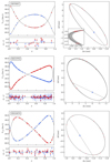 |
Fig. 3. Same as Fig. 2, but for the system HD 70937, HD 210763, and HD 224974 from top to bottom, respectively. |
4.5. HD 210763
The first RV observations of this system were performed at Mount Wilson Observatory and published by Wilson & Joy (1950) who already noticed the variability of the velocities. The double-line signature was later detected by Nadal et al. (1983) who determined the first spectroscopic orbit. With new observations from the Observatoire de Haute Provence, they determined a period of 42.4 d and an eccentricity of 0.616. The spectral type of the primary is between F8 IV and F6 V. Fekel et al. (2011) revised the spectroscopic orbit with extensive new and more precise RVs. They also classified the spectral type of the two components to be F6 V and F6 IV. They measured a mass ratio q = 0.855 ± 0.003. We used their RVs together with ours derived from the UVES spectra. We corrected our RVs by −0.1 km s−1 due to a RV offset.
We displayed our combined fit in Fig. 3. We have a very precise astrometric orbit with a rms of ∼15 μas. The masses were measured with an accuracy of 0.26%, with the same mass ratio as Fekel et al. (2011). Our measured orbital parameters are listed in Table 6. We measured a K-band flux ratio of 37.1 ± 0.8%, and an orbital parallax of 10.691 ± 0.037 mas. We reached a similar precision as Gaia, which is in disagreement by 2.3σ with our measurements.
4.6. HD 224974
This system is composed of twin main-sequence stars orbiting each other with a 10.7 d period. The full spectroscopic orbital solutions were determined by Gorynya & Tokovinin (2014), who derived a mass ratio of q = 0.982 ± 0.003. This is consistent with the previous estimate of 1.000 ± 0.011 from the GCS.
We present in Fig. 3 our combined fit using only our new RVs determined from UVES and HARPS spectra. Our astrometric orbit is precise at a 11 μas level. We measured the masses with an accuracy of 0.5%, providing a mass ratio q = 0.981 ± 0.007, which is in very good agreement with Gorynya & Tokovinin (2014). Our measured distance is accurate at 0.3% and at 2.1σ with the Gaia value. The fitted parameters are listed in Table 6. We also measured an average K-band flux ratio of 90.0 ± 0.9%.
4.7. HD 188088
This star is a BY Dra variable and a member of a triple system containing an inner spectroscopic binary and an outer M5 companion. The third component is, however, located at about 41″ (Allen et al. 2012; Chini et al. 2014) and therefore has a negligible impact on the inner system we are studying here. The spectroscopic components have a similar brightness with spectral type K3V and orbit each other in 46.8 d. The first spectroscopic observations were acquired by Evans (1968) who suggested the binary nature of the system. This was later confirmed by Fekel & Beavers (1983) who detected the lines of both components and determined the first spectroscopic orbital solutions. They were then refined by Fekel et al. (2017) with new and more precise RVs. They estimated a minimum mass of 0.86 M⊙ for both stars.
Our orbital fit is displayed in Fig. 4 and the solutions are listed in Table 6. We only used our more precise and uniform HARPS and UVES observations to avoid additional offsets (there is no improvement in precision by adding the RVs from Fekel et al. 2017). A zero-point offset of +0.039 km s−1 was added to the HARPS measurements. We reached a final rms of the orbit of ∼18 μas. We measured the masses and the distance with a precision of ∼0.03%. Our mass ratio is in agreement at 0.05σ with Fekel et al. (2017). The Gaia parallax is at 3.0σ with our value and we reached a better accuracy. We also measured an average K-band flux ratio of 90.1 ± 1.6%.
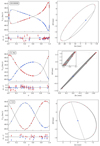 |
Fig. 4. Same as Fig. 2, but for the system HD188088, LL Aqr, and o Leo from top to bottom, respectively. |
4.8. LL Aqr
This is a well-studied detached eclipsing system composed of main-sequence stars (F9V + G3V, Graczyk et al. 2016) orbiting each other in 20.2 d. First discovered as being variable by the HIPPARCOS mission, the first combined photometric and RV solution was obtained by Ibanoǧlu et al. (2008). The orbital parameters and absolute dimensions were later refined with new and more precise measurements. The latest data set was provided by Graczyk et al. (2016), who determined the masses with a precision of 0.06% and a distance precise at 3%. We used their RVs in our combined fit.
Our orbital solutions are displayed in Fig. 4 and the fitted parameters are listed in Table 6. We reached the same level of precision as Graczyk et al. (2016) for the masses. In addition, our values are in very good agreement with theirs at the < 0.3σ level, demonstrating the accuracy of the measurements as well. Our distance has a better accuracy with 0.27%, but it is still in agreement with their value. Our distance uncertainty is similar to Gaia and is in agreement at 0.9σ. We also measured an average K-band flux ratio of 53.3 ± 0.7%.
4.9. o Leo
This system is composed of a F8-G0 giant star and a hotter A7m III−IV companion, as identified by Ginestet & Carquillat (2002). Hummel et al. (2001) presented the first three-dimensional solution by combining photoelectric RVs and astrometry from interferometry. They measured M1 = 2.12 ± 0.01 M⊙, M2 = 1.87 ± 0.01 M⊙, and d = 41.4 ± 0.1 pc. The composite spectra were more deeply studied by Griffin (2002) who determined effective temperatures of 7600 K and 6100 K for the giant and dwarf component, respectively. Piccotti et al. (2020) updated the orbit with new RVs from Massarotti et al. (2008) and measured M1 = 2.093 ± 0.068 M⊙ and M2 = 1.857 ± 0.058 M⊙.
We obtained new UVES spectroscopic and interferometric data to improve the solutions and to obtain more precise masses and distances. We also complemented the RVs with archived SOPHIE spectra. We found a zero-point offset of −0.098 km s−1 for SOPHIE. As we can see in Fig. 4, we obtained a very precise orbit, with an average rms of ∼10 μas, demonstrating that the 20 μas systematic error we added (see Table 4) is probably too conservative. We measured the masses with a precision of 0.6%, which are in agreement at < 0.3σ with Piccotti et al. (2020). However, they differ from Hummel et al. (2001) by ∼2 − 3σ. We fitted their RVs with our astrometry and we also found the masses to be in disagreement by about the same amount. We performed the same check with the RVs from Massarotti et al. (2008) and found the masses to be in agreement within 1σ with our measurements. We therefore suspect that the disagreement with the Hummel et al. (2001) masses comes from their photoelectric RVs.
We measured a distance of 40.964 ± 0.135 pc, which is in agreement within 1σ with Piccotti et al. (2020) but at 3σ with Hummel et al. (2001). It is also consistent at 0.7σ with Gaia.
For each epoch, we were able to measure the uniform-disk (UD) angular diameter of the primary component as it is large enough to be spatially resolved. We measured an average value of θUD1 = 1.285 ± 0.075 mas. We converted this value to a limb-darkened (LD) angular diameter using a linear-law parametrisation Iλ(μ)=1 − uλ(1 − μ). The LD coefficient uλ = uK = 0.1956 ± 0.0265 (Claret & Bloemen 2011, we took the mean and standard deviation of the coefficient given by the least-square and flux conservation methods) was chosen taking the stellar parameters as close as possible to the values listed in Table 7. The conversion is then given by the approximate formula of Hanbury Brown et al. (1974):
which gives θLD, 1 = 1.303 ± 0.076 mas. It is in agreement with the 1.31 ± 0.23 mas determined by Hummel et al. (2001). We also estimated an average flux ratio in K of 25.03 ± 0.20%, which is also in excellent agreement with 25.4 ± 1.2 measured by Hummel et al. (2001).
4.10. V963 Cen
This is a thoroughly studied high-eccentricity solar-type eclipsing system composed of two G2V-IV stars (Graczyk et al. 2022). First discovered as likely being variable by Olsen (1993), the first photometric measurements covering the eclipses were only obtained later by Clausen et al. (1999, 2001) who refined the orbital period. The first orbital solutions combining both photometry and spectroscopy were obtained by Sybilski et al. (2018) who measured masses precisely at a 0.08% level. In Graczyk et al. (2022), we refined the solutions by using more precise photometry from the Transiting Exoplanet Survey Satellite (TESS; Ricker et al. 2014) and new HARPS observations. We also noticed an apsidal motion of about 55 000 yr, but in our case this is negligible as the time span by our data set is small.
In our combined fit displayed in Fig. 5, we used the RVs of Graczyk et al. (2022), which are the most precise and they were also determined with the broadening function method from the RaveSpan software. We measured the masses at a 0.08% precision and the distance at 0.2%. Our masses are in good agreement with those measured by Graczyk et al. (2022) at a ∼0.5σ level, but they are in slight agreement (∼2σ) with Sybilski et al. (2018). However, they assumed a fixed eccentricity in their fitting process which likely results in underestimated uncertainties because the masses are directly linked to the eccentricity such that M ∝ (1 − e2)3/2. As a check, we combined our astrometry with their RVs and found an agreement at 1.1σ with our values. In addition, RVs from Sybilski et al. (2018) are less precise and accurate than ours, providing a reduced χ2 of the secondary RVs larger ( ) than ours (
 ).
).
Our distance is also in agreement within 1σ with the photometric distance estimated by Graczyk et al. (2022), and at 0.8σ from Gaia. We measured a flux ratio in K of 96.0 ± 1.1%, consistent with the extrapolated value of Graczyk et al. (2022).
5. Evolutionary state
We employed the same fitting method as in Gallenne et al. (2016, 2018b, 2019), that is to say we used several stellar evolution models. We fitted the PARSEC (PAdova and TRieste Stellar Evolution Code, Bressan et al. 2012), BaSTI (Bag of Stellar Tracks and Isochrones, Pietrinferni et al. 2004), MIST (Mesa Isochrones and Stellar Tracks, Choi et al. 2016), and DSEP (Dartmouth Stellar Evolution Program, Dotter et al. 2008) isochrone models to estimate the stellar age of our systems. These models are well suited for our targets as they include the horizontal and asymptotic giant branch evolutionary phases, and contain a wide range of initial masses and metallicities. In addition, it enable us to test the uncertainty of the age induced by different models.
PARSEC models are computed for a scaled-solar composition with Z⊙ = 0.0152, and they follow a helium initial content relation Y = 0.2485 + 1.78Z with a mixing length parameter αMLT = 1.74. They include convective core overshooting during the main sequence phase, parametrised with the strength of convective overshooting in units of the pressure scale height lov = αovHp. The overshooting parameter αov is set depending on the mass of the star, that is αov = 0 for M ≲ 1.1 M⊙, αov ∼ 0.25 for M ≳ 1.4 M⊙, and linearly ramps with the mass in between. The BaSTI models are computed for a scaled-solar composition with Z⊙ = 0.0198, following the relation Y = 0.245 + 1.4Z with αMLT = 1.913. They also include convective core overshooting with the same parametrisation, but with the conditions αov = 0 for M ≲ 1.1 M⊙, αov = 0.20 for M ≳ 1.7 M⊙, and (M − 0.9 M⊙)/4 in between. The MIST models use a scaled-solar composition with Z⊙ = 0.0142, with the relation Y = 0.2703 + 1.5Z and αMLT = 1.82. They use an alternate prescription of the core overshooting with a diffusion coefficient Dov = D0exp( − 2z/Hν), where z is the distance from the edge of the convective zone, D0 is the coefficient at z = 0, and Hν is defined with the overshooting parameter fov such that Hν = fovHp. MIST models adopt a fixed value fov = 0.016 for all stellar masses, which would be approximatively converted to αov ∼ 0.18 (Claret & Torres 2017). The DSEP models use a scaled-solar composition with Z⊙ = 0.0166, with the relation Y = 0.245 + 1.5Z and a solar-calibrated mixing length αMLT = 1.938. The amount of core overshooting is also parametrised as a multiple of the pressure scale height such as, for solar metallicity, αov = 0.05, 0.1, and 0.2 for M ≲ 1.2 M⊙, 1.2 M⊙ < M < 1.3, and M ≳ 1.3 M⊙, respectively.
We retrieved several isochrones from the PARSEC database tool10, with ages ranging from log t = 6.6 to 10.13 with a step of 0.05 (i.e. ∼0.005 − 13 Ga), and metallicities from Z = 0.003 to 0.06 (i.e. −0.7 ≤ [Fe/H] ≤ +0.6, using [Fe/H]∼log(Z/Z⊙)), with a step of 0.001 (fine enough to avoid re-interpolation). The BaSTI isochrones are pre-computed in their database11, we downloaded models for t = 0.1 − 9.5 Ga by a step of ∼0.2 Ma and Z = 0.002, 0.004, 0.008, 0.01, 0.0198, 0.03, and 0.04 (i.e. −1.0 ≤ Fe/H ≤ 0.3). For fitting purposes, we created an interpolated grid of the BaSTI isochrones in Z, from 0.002 to 0.04 with a step of 0.001. We also computed MIST isochrones from their database tool12 using the standard age grid from 0.1 Ma to 20 Ga with a step of ∼1 Ma, and for metallicities in the range 0.001 ≤ Z ≤ 0.045 (i.e. −1.15 ≤ Fe/H ≤ 0.5) with a step of 0.001. We downloaded DSEP isochrones from their website13 with a grid with an age from 1 Ga to 10 Ga with a step of 0.02 Ga and metallicity from 0.001 to 0.058 with a step of 0.001 (i.e. −1.2 ≤ Fe/H ≤ 0.5).
When possible, we searched for the best-fit age in stellar effective temperature, radius, mass, and K-band absolute magnitude for both components simultaneously, assuming coeval stars and following χ2 statistics:
![Mathematical equation: $$ \begin{aligned} \chi ^2 = \sum _{i=1}^2 \left[ \left(\dfrac{\Delta T_{\rm eff}}{\sigma _{{T}_{\mathrm{eff}}}}\right)_i^2 + \left(\dfrac{\Delta R}{\sigma _R}\right)_i^2 + \left(\dfrac{\Delta M}{\sigma _M}\right)_i^2 + \left(\dfrac{\Delta M_{K}}{\sigma _{M_{K}}}\right)_i^2 \right], \end{aligned} $$](/articles/aa/full_html/2023/04/aa45712-22/aa45712-22-eq13.gif)
where the sum is over both components (i = 1, 2). The Δ symbol represents the difference between the predicted and observed quantities. The effective temperature and the radii are measured quantities and were taken from the literature. They are listed in Table 7. The masses were also measured for this work and are reported in Table 6. When available, we took care of re-scaling the retrieved linear radii according to our own estimate of the linear semi-major axis. In our isochrone plots, we also display the stellar luminosity estimated from the Stefan-Boltzmann law, but this parameter was not included in the fit as this is not an independent measurement. Absolute magnitudes in the K band, MK, were also included in the fit using our measured flux ratio fK following the relations
Stellar parameters used for the age determinations, together with our fitted and adopted age for the systems.
 (1)
(1)
 (2)
(2)
where mK is the combined magnitude as measured in the 2MASS catalogue (Cutri et al. 2003), d our measured distance, and AK the extinction coefficient in the K band, such as AK = 0.119 AV (Fouqué et al. 2007) and AV = 3.1E(B − V) (Cardelli et al. 1989). The colour excess coefficient was estimated from the three-dimensional extinction map STILISM14 (Lallement et al. 2018). It is worth mentioning that our systems are nearby and the effect of reddening is generally negligible. All errors have been propagated to the final magnitudes.
The stellar metallicity was kept fixed in the fitting process to a value from the literature (listed in Table 7). Our fitting procedure was the following. For all isochrone models, we first chose the closest grid in Z for a given metallicity. Then, we searched for the global χ2 minimum in age by fitting all isochrones for that given metallicity. A second fit was then performed around that global minimum value, and where the grid was interpolated in age at each iteration. To assess the uncertainties on the four isochrone models (i.e. PARSEC, BaSTI, MIST, and DSEP), we repeated the process with Z ± σ. Our final adopted age corresponds to the average and standard deviation between the four models.
AK For. We adopted the metallicity from Hełminiak et al. (2014) and the stellar parameters (effective temperatures, radii, and flux ratio in K) listed in Table 7. All models give a rather different estimate for the age, although all values are within 1σ. PARSEC gives a substantially younger system compared to the other models and the predicted masses are > 30σ away from our measurements. The best model (i.e. the one with all parameters within 1 − 2σ) is from BaSTI isochrones with all predicted stellar parameters within 1σ, giving an age of 9.5 ± 0.01 Ga. This is older than the 6 Ga estimated by Hełminiak et al. (2014) using DSEP isochrones, although there is no error quoted by the authors. However, it would be in agreement within errors with our DSEP fit. Excluding the age estimated with PARSEC, we adopted an average age of 7.9 ± 1.3 Ga. As displayed in Fig. 6, all models show that both stars still reside on the main sequence, which is in agreement with previous works, and that they are near the turnoff point. Using the stellar temperatures and adopting the spectral type-temperature calibration of Pecaut & Mamajek (2013), we determined that the primary and the secondary component have spectral types of K4V and K5V, respectively, with a ±1 index as uncertainty due to the temperature errors.
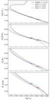 |
Fig. 6. Fitted PARSEC, BaSTI, MIST, and DSEP isochrones for the AK For system. We note that the luminosities were not fitted and were estimated from the Stefan-Boltzmann law. |
HD 9312. The metallicity 0.03 ± 0.1 dex from Kiefer et al. (2018) was used for the isochrone fit. As observables, we used their measured effective temperatures, our measured masses, and K-band flux ratio. Luminosities and radii can also be estimated using our measured masses, as well as the temperatures and surface gravities from Kiefer et al. (2018). However, they are not independent parameters, so they are displayed in Fig. E.1 but not included in the isochrone fit.
We found a system that is slightly younger than Wang et al. (2015), that is the secondary still resides on the main sequence while the primary is exiting the turnoff point. This is because the work of Wang et al. (2015) is based on the primary star properties only (SB1 at that time), a solar metallicity Z = 0.019, and a larger estimate (∼15%) of the mass ratio compared to our measurement (q = 0.763) and the one from Halbwachs et al. (2014, q = 0.762). We see in Fig. E.1 that all models provide an acceptable fit of the observations, although they all provide a secondary effective temperature that is larger by ∼1.5σ, while the primary temperature is within 1σ except for the PARSEC model. To reconcile the observations with the models within 1 − 2σ, we would need to increase the measured metallicity to 0.1 dex. However, the PARSEC models still predict masses > 3σ. The best agreement is given by DSEP and MIST, but all give a similar age for the system (see Table 1). We adopted an average age of 5.60 ± 0.09 Ga. There are no significant changes if we choose the same metallicity [Fe/H] = 0.1 dex as Wang et al. (2015), with all isochrones giving a similar age. As previously mentioned, using the calibration from Pecaut & Mamajek (2013), we determined the spectral types to be G9V and K1V for the primary and secondary star, respectively.
HD 41255. There are neither measurements for the effective temperature nor metallicity for this system. The temperature can be estimated from colour-temperature calibrations (using the (V − K) colour for instance; see e.g. Casagrande et al. 2011). However, measured magnitudes include the flux from both components. To estimate the individual magnitudes in K, we used our measured flux ratio and Eqs. (1) and (2). We used the same equations for the V band, assuming the same flux ratio as in K. We estimated an average effective temperature Teff, 1 = 6107 ± 39 K and Teff, 2 = 5984 ± 39 K combining the (V − K)−Teff, relations from di Benedetto (1998), Houdashelt et al. (2000), Ramírez & Meléndez (2005), Masana et al. (2006), González Hernández & Bonifacio (2009), and Casagrande et al. (2010). As the flux ratio is close to 1, we found similar temperatures between the stars (error is the standard deviation between the relations). This is consistent with 5996 ± 330 K estimated by Gaia (assuming a single star).
To go a step further, we disentangled our UVES spectra and estimated the effective temperatures. For disentangling, we used all spectra with the RaveSpan software which utilises the method presented in González & Levato (2006). We ran two iterations choosing a median value for the normalisation of the spectra. We then performed a spectral analysis using the Stellar Parameters And Chemical abundances Estimator code SP_Ace15 (Boeche & Grebel 2016). This tool employs a new method based on a library of general curve-of-growth (GCOG) in the spectral range 4800 − 6860 Å. Stellar parameters were derived from a χ2 minimisation between the observed and model spectra. However, SP_Ace neither relies on a library of synthetic spectra, nor does it measure the equivalent width (EW) of absorption lines, but it constructs the models from a library of GCOG, which are coefficients of polynomial functions (one per absorption line) describing the EW of the lines as a function of the stellar parameters (for more details, see Boeche & Grebel 2016). This tool uses different elements such as Fe, C, N, O, Mg, Al, Si, Ca, and Ti (up to 21 elements) to estimate the stellar parameters Teff, log g, [M/H], and elemental abundances. We found for the primary component Teff = 6017 ± 120 K, log g = 4.46 ± 0.18 dex, and [Fe/H] = −0.21 ± 0.08 dex. The temperature is similar to the one predicted by colour-temperature calibrations. The uncertainties were estimated by repeated the process by fixing the temperature to values of ±200 K, and fixing log g to ±0.25 dex. A comparison of the observed average spectrum and the fitted SP_Ace model is displayed in Fig. 7.
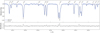 |
Fig. 7. Comparison of the decomposed primary spectrum (blue line) with the synthetic spectrum (red line) for the binary system HD 41255. |
We performed the same spectral analysis for the secondary component. We found Teff = 6064 ± 98 K, log g = 4.57 ± 0.21 dex, and [Fe/H] = −0.09 ± 0.07 dex. The metallicity of the two components is within ∼1σ of each other, we therefore adopted an average and standard deviation of [Fe/H] = −0.15 ± 0.06 dex for the system. This is at 1σ with the −0.17 dex derived from the colour-[Fe/H] calibration of the GCS, although assuming a single star.
From the isochrone fit, we found the system to be composed of two main-sequence stars near the turnoff point. Isochrones are displayed in Fig. E.1. The BaSTI and DSEP models give a similar age, although BaSTI better fits all the observables (< 2.2σ difference). We adopted an average age between these two models of t = 2.57 ± 0.14 Ga. We also estimated the luminosity and radius of both components using log g, Newton’s law of gravitation, and the Stefan-Boltzmann law. They are also listed in Table 7 but they are not included as fitted parameters. The PARSEC and MIST isochrones are not reliable as they provide a system that is too young, < 600 Ma. Our estimate is smaller than the value reported by Casagrande et al. (2011) from a Bayesian analysis of isochrone matching based on temperature and metallicity relations. Assuming a single star, they derived  Ga using the PARSEC models and
  Ga with BaSTI. We note that their inferred mass is also not consistent with our measurement at > 2σ. The GCS survey also predicted a higher age of
  Ma from fitting the PARSEC isochrone with their effective temperature of 6081 K determined from the IR flux method, a metallicity of −0.17 dex, and the Hipparcos distance to estimate the absolute magnitudes. In general, we can see in Fig. E.1 that the isochrone models predict a slightly higher temperature of about +200 K. From the measured temperatures, we derived the spectral types to be F9V for both stars.
HD 70937. No measurements of the effective temperature nor metallicity is available in the literature. The average temperature given by colour-temperature relations cited previously is 6401.2 + / − 79.3 K for both components, using the same flux ratio in V as in K. We also estimated the stellar parameters from our UVES disentangled spectra following the same analysis as previously discussed using both SP_Ace codes. For the primary star, we estimated Teff = 6277 ± 100 K, log g = 3.72 ± 0.27 dex, and [Fe/H] = −0.02 ± 0.06 dex, and then Teff = 6446 ± 84 K, log g = 4.10 ± 0.24 dex, and [Fe/H] = 0.05 ± 0.06 dex for the secondary. We adopted an average metallicity of 0.02 ± 0.04 dex for the system. All parameters are reported in Table 7.
We found that both stars are at the main-sequence turnoff, as shown in Fig. E.2. We also display the luminosity and radii as calculated previously, but they are not fitted. All models provide a similar age for the system, with BaSTI being the best fitted model. The most discrepant parameters are the temperature, which is higher by 2 − 5σ. To reconcile the models within 1 − 3σ, we would need to increase the measured metallicity to 0.1 dex at 2.5σ with our measured value. We adopted the average value of 1.78 ± 0.07 Ma as the age of the system. This is in agreement with 1.5 ± 0.1 Ma derived by Holmberg et al. (2009) from the GCS, although they used a temperature of 6412 K and a [Fe/H] = 0.01 dex. From the measured temperatures, we determined the spectral types to be F7V and F5V for the primary and secondary, respectively.
HD 210763. There is no measurements of the temperatures or metallicity in the literature. The colour-temperature relations predict an average temperature around 6250 K for both stars (also assuming the same flux ratio in V as in K). Using the SP_Ace code on the disentangled spectra, we measured Teff = 6173 ± 38 K, log g = 3.78 ± 0.26 dex, and [Fe/H] = −0.03 ± 0.07 dex for the primary star, and Teff = 6523 ± 87 K, log g = 4.08 ± 0.29 dex, and [Fe/H] = 0.04 ± 0.06 dex for the secondary component. We adopted an average metallicity of 0.01 ± 0.04 dex, which is in agreement with the predicted value of 0.05 from Holmberg et al. (2009).
As for HD 70937, both stars are located at the main-sequence turnoff, as shown in Fig. E.2. All models provide a similar age for the system, with BaSTI best fitting the data with the lowest  . We adopted an average age of 1.67 ± 0.07 Ma (excluding MIST). This is similar to Holmberg et al. (2009) predicting 1.3 ± 0.2 Ma. We note that all models provide temperatures that are > 3σ with the measurements. Increasing the metallicity to 0.1 dex would mitigate the discrepancy within 2σ for the BaSTI and PARSEC models. Our final stellar parameters are listed in Table 7. We derived their spectral type to be F8V and F5V.
HD 224974. We performed the same analysis with SP_Ace for this system as there are no measured temperatures or metallicities in the literature. The colour-temperature relations predict an average temperature around 6141 K for both stars (assuming the same flux ratio in V as in K). The SP_Ace analysis provides Teff = 6221 ± 85 K, log g = 4.33 ± 0.13 dex, and [Fe/H] = 0.16 ± 0.05 dex for the primary star, and Teff = 6171 ± 75 K, log g = 4.49 ± 0.20 dex, and [Fe/H] = 0.07 ± 0.07 dex for the secondary. We adopted an average metallicity of 0.04 ± 0.03 dex, which is in agreement with the predicted value of 0.08 from Holmberg et al. (2009).
Our isochrone fit of Fig. E.3 shows that both stars exhausted the hydrogen fuel at their cores and are entering the turnoff point. We obtained the best fitted isochrone with the BaSTI models, with all parameters within 1.5σ, while MIST and PARSEC are not consistent, providing a system that is too young, < 600 Ma. All parameters are reported in Table 7. We adopted t = 2.98 ± 0.07 Ga as a final age for the system, corresponding to the average value between the BaSTI and DSEP models. This is consistent with the predicted value of 2.4 ± 0.2 from the GCS. We derived their spectral type to be F7V and F8V.
HD 188088.Gray et al. (2006) measured a metallicity of 0.29 dex, log g = 4.24, and a temperature of 4774 K, assuming a single star. Luck (2017) measured a lower metallicity of 0.12 dex (although within 1σ), while their temperature of 4818 ± 63 K and surface gravity og 4.20 dex are similar to Gray et al. (2006). We did not succeed in converging with SP_Ace on our average disentangled spectrum because it reached the upper limit metallicity range of 0.5 dex. This may be due to the fact that the stars are chromospherically active, with light variability due to star spots, which can prevent a good spectral disentangling. Boeche & Grebel (2016) succeeded in using SP_Ace with a FEROS spectrum and determined Teff = 4868 ± 80 K, log g = 3.50 ± 0.03 dex, and [Fe/H] = −0.32 ± 0.38 dex. The temperature is in good agreement with the previous authors, while the surface gravity is lower. The metallicity, however, is inconsistent with previous estimates. In our isochrone fit, we adopted the mean temperature and gravity of 4820 K and 4.00 dex for both stars, and considered 200 K and 0.3 dex as uncertainty, respectively. For the metallicity, we tested different values in the range [−0.35, 0.35] dex that match the measurements best.
We found that the best fit of the isochrone models is given for a metallicity of 0.28 dex. However, the masses are still > 8σ for all models, except for BaSTI. The most acceptable fit is with BaSTI providing predicted values at < 2σ from the measurements, except M2 at ∼5σ. However the given age of 910 Ma is too young for such stars. The other models predict masses > 8σ, with rather different ages and large uncertainties. We adopted the average age t = 1.6 ± 1.1 Ga as it is not possible to constrain it better. The isochrones are displayed in Fig. E.3 and the stellar parameters are with fitted ages in Table 1. This system is a good example of not being able to constrain the age even with very accurate mass measurements, demonstrating the importance of the other stellar parameters.
LL Aqr. We used the metallicity, temperatures, radii, and the V-band flux ratio determined by Graczyk et al. (2016). The luminosity was also used, but not fitted as explained previously. Our isochrone fits of Fig. E.4 show that both stars are near the main-sequence turnoff. All models provide a consistent age with each other; however, no model satisfies all observables at less than 3σ. All isochrones are too hot with respect to the measurements. This was also noticed by Graczyk et al. (2016) who used the PARSEC and MESA (Modules for Experiments in Stellar Astrophysics, Paxton et al. 2015) isochrones. To mitigate the discrepancy, the metallicity would need to increase to ∼0.15 dex, which is at 3σ with the measured value. Instead, Graczyk et al. (2016) reconciled the predicted and observed parameters by fine-tuning some internal stellar parameters of the stellar evolutionary tracks, more particularly the element diffusion and allowing for different mixing-length parameters for the two components. They estimated an age for this system ranging from 2.3 to 2.7 Ga, which agrees with our average value of 2.76 ± 0.20 Ga; although, the four models do not match the observables properly.
o Leo. The metallicity and temperature of the giant star (primary) were estimated by Adamczak & Lambert (2014) from new high-resolution spectra. They determined Teff = 6173 ± 59 K, log g = 3.06 ± 0.25 dex, and [Fe/H] = −0.06 ± 0.09 dex. This is consistent with 6200 ± 200 K reported by Griffin (2002), who also determined the secondary effective temperature to be 7600 ± 200. We performed a SP_Ace analysis with our disentangled spectra of the primary and estimated Teff = 6107 ± 93 K, log g = 2.91 ± 0.24 dex, and [Fe/H] = 0.11 ± 0.10 dex, in good agreement with the previous study. For the secondary, we could not use the SP_Ace algorithm because the effective temperature is not in the stellar parameter ranges covered (3600 K < Teff < 7400 K). We therefore adopted the temperature estimated by Griffin (2002). As for HD 9312, we can have an estimate for the secondary radius via Stefan’s law and our measured primary radius. We assumed a bolometric flux ratio of 0.43 ± 0.04, similar to the measured flux ratio measured by Hummel et al. (2001) at 0.55 μm.
Our isochrone fit is displayed in Fig. E.4. We note that L1, L2, and R2 are displayed but not fitted as they are not independent parameters. All models provide a similar age, except for MIST, giving an average age of 1.06 ± 0.03 Ga (excluding MIST). BaSTI and PARSEC best fit the observables within 2.5σ. The MIST model predicts a younger system than the other models. Our derived age is in good agreement with the 1.02 Ga determined by Griffin (2002) assuming a metallicity Z = 0.02 dex. In agreement with the previous works, we see that the primary is a giant and the secondary is a dwarf star located at the turnoff point.
V963 Cen. We used the metallicity, temperatures, and radii determined by Graczyk et al. (2022). The luminosity was also used but not fitted as explained previously. Our isochrone fits of Fig. E.5 show that both stars are near the main-sequence turnoff. Although all models provide a similar age of 6.10 ± 52 dex, none gives a consistent fit, with most of the parameters above 3σ with the predicted values. The models predict slightly hotter components with the given metallicity [Fe/H] = −0.06 ± 0.05 dex. To reconcile the isochrones within 1−2σ with the same stellar effective temperatures (which are easier to measure than the metallicity), we tested different metallicities. To reconcile the BaSTI and MIST isochrones, we would need a metallicity of ∼0.13 dex, while ∼0.1 dex would reconcile the BaSTI models. We did not find an acceptable metallicity to better match the PARSEC models. A metallicity of ∼0.1 dex would provide slight agreement for some observables, but the masses and secondary radii are > 5σ away.
In Fig. E.5, we display the isochrones for two metallicities, −0.06 dex as estimated in Graczyk et al. (2022) and 0.1 dex, which better fit the observables. They give an age of 6.15 ± 0.31 Ga and 7.31 ± 0.06, respectively. The stellar parameters are reported in Table 7, together with the age given for each model for the second metallicity.
6. Comparison with Gaia parallaxes
We compared our measured orbital parallaxes from this study and from our previous works (Gallenne et al. 2016, 2018b, 2019) with the Gaia third data release (Gaia Collaboration 2023). We applied a zero-point offset to each Gaia value following the correction recipe from Lindegren et al. (2021a). As we can see in Fig. 8, we found that ∼50% (8/16) of the sample is more than 1σ away.
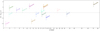 |
Fig. 8. Comparison of our orbital parallaxes with the Gaia DR3 measurements. |
To check if Gaia would detect the astrometric signature of the primary star around the centre of mass, that is to say the influence of the secondary star on the primary, we calculated a S/N as follows:
 (3)
(3)
 (4)
(4)
where aphot is the photocentre semi-major axis related to the angular semi-major axis a, the mass of the components M1, M2, and the magnitude difference ΔmV = m2 − m1. While σfov = 34.2 μas is the along-scan accuracy per field of view crossing as defined by Perryman et al. (2014, we adopted the value for stars with G < 10 mag). We estimated the magnitude difference between the components using our previously fitted isochrone models, and in the V band as it is similar to the Gaia G band. We list in Table 8 the value of aphot and S/N for each star studied here and previously. We also mention the corresponding Gaia Renormalized Unit Weight Error (RUWE), which is the square root of the normalised χ2 of the astrometric fit to the along-scan observations. This parameter is a good metric to distinguish between a good or bad single-star astrometric solution, whose threshold is usually set to be around 1.4.
Additional information about the systems and their detection with Gaia.
First, we notice that most systems have a large S/N and they will be detected by Gaia in the next data release (DR). DR3 provides results for about 800 000 binary stars, including solutions for astrometric, spectroscopic, and eclipsing binaries (Gaia Collaboration 2023; Halbwachs et al. 2023). Unfortunately, only the known eclipsing system AK For has published full orbital solutions, with a corrected parallax improving the agreement with our measurement from 0.7σ to 0.6σ. However, their given eccentricity of 0.287 ± 0.098 is not at all consistent with the zero eccentricity we measured or previously published. This discrepancy likely comes from the fact that the Gaia solutions only fitted the astrometry, which poorly constrained some orbital parameters of eclipsing systems (as seen with the given eccentricity precision). Combined fits generally provide more robust solutions. DR4 should contain orbital solutions for all available binary stars, including those presented here as they have a large astrometric S/N, and our precise results will likely provide the best reference systems to test and validate the Gaia solutions. The systems HD 70937, HD 224974, V963 Cen, TZ For, AI Phe, and AL Dor are also listed in the Gaia DR3 non-single star catalogue, but no astrometric solutions are derived.
In the top and bottom panel of Fig. 9, we plotted the RUWE parameter with respect to the relative parallax difference and the semi-major axis of the photocentre aphot, respectively. As we previously mentioned, a threshold of RUWE ≲ 1.4 is usually used to indicate well-behaved Gaia solutions (Lindegren 2018; Lindegren et al. 2021b), which we show with a dotted vertical line. We see that the stars with the largest RUWE (ψ Cen, HD 9312, and o leo) have the largest S/N (> 15), for which we may think the Gaia parallax is the most biased and less reliable. This is, however, not the case because the agreement with our measurements is ≤2σ (0.6, 1.8, and 0.7σ, respectively). Those stars also have the largest photometric semi-major axis, but they still provide a consistent parallax. The most discrepant Gaia parallaxes are in the ‘good’ RUWE range 1.0 − 1.4. This has already been reported by Stassun & Torres (2021), who compare the Gaia parallaxes with benchmark eclipsing binaries and show that the RUWE is highly sensitive to unresolved companions. They also report a correlation with the photocentre semi-major axis, which we also see in the bottom panel of Fig. 9. As Stassun & Torres (2021) and Kervella et al. (2022) suggested, a RUWE slightly larger than one may imply the presence of unseen binaries.
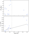 |
Fig. 9. Correlations between the RUWE metric, the absolute fractional parallax difference (top), and the photocentre semi-major axis of the systems (bottom). The solid line is the linear correlation law estimated by Stassun & Torres (2021). The dotted vertical line denotes RUWE = 1.4. |
7. Conclusions
We have reported new interferometric and spectroscopic observations of double-lined binary systems. We simultaneously fitted the astrometry and RVs to obtain extremely precise and accurate masses and distances for ten systems. We reached uncertainties as low as 0.03% and an average precision of ∼0.2%. A comparison with previous studies and different datasets demonstrated that our measurements are both precise and accurate. This was possible thanks to the precision and sensitivity of the GRAVITY instrument, which provided exquisite differential astrometry, with a median rms of ∼16 μas.
We confronted our measurements with additional observables to four stellar evolution models and we show that theory is clearly deficient for most of the systems when fitting one common isochrone for the components in a system. We estimated an average age for the system taking into account the uncertainty on the metallicity and the scatter between the ages given by each model. In four cases, the models give a different age for a given system and this may lead to a wrong estimate when using a single evolution model. To reconcile the models, it is likely that a fine-tuning of the models of each star in a given system is necessary, as was done by Graczyk et al. (2016). With such precision as to the masses, stellar interior parameters such as the mixing length and envelop overshooting can now be better constrained and lead to an improved calibration of stellar evolution models.
Our very precise orbital parallaxes also provide a stringent test of Gaia measurements. We found that 50% (8/16 stars, including our previous works) of our sample is > 1σ away from the Gaia parallax, and within the ‘nominal’ RUWE range 1 − 1.4. This can be problematic for stars with unresolved companions which would bias the parallax. We also confirm the correlation between the photocentre semi-major axis and the RUWE parameter reported by Stassun & Torres (2021), that is to say the larger the photocentre motion is, the larger the RUWE. This is somewhat expected for large RUWE, meaning the poorly constrained Gaia 5- and 6-parameter astrometric solutions, but not for RUWE < 1.4 which is the frequently used cutoff for reliable Gaia astrometry. To reconcile most of the Gaia parallaxes within 1σ with our measurements, we need to inflate the Gaia errorbars by a factor of two. Several other systems are being observed and will provide a large sample of benchmark stars with high-precision masses and distances.
Available at http://www.jmmc.fr/searchcal
Available at https://github.com/amerand/CANDID
The offset of the fibres can be extracted from the header of the fits files with the keyword ESO QC MET SOBJ DRAX and ESO QC MET SOBJ DDECX where X = 1, 2, 3, or 4.
With the Python package emcee developed by Foreman-Mackey et al. (2013).
Acknowledgments
We thank F. Widmann and J. Stadler for making public the code to create the GRAVITY aberration maps. A.G. acknowledges the support of the French Agence Nationale de la Recherche (ANR), under grant ANR-15-CE31-0012-01 (project UnlockCepheids). A.G. also acknowledges financial support from the ANID-ALMA fund No. ASTRO20-0059. The research leading to these results has received funding from the European Research Council (ERC) under the European Union’s Horizon 2020 research and innovation programme under grant agreement No. 695099 (project CepBin), No. 951549 (project UniverScale) and from the National Science Center, Poland grants MAESTRO UMO-2017/26/A/ST9/00446 and BEETHOVEN UMO-2018/31/G/ST9/03050. B.P. acknowledges support from the Polish National Science Center grant SONATA BIS 2020/38/E/ST9/00486. We also acknowledge support from the Polish Ministry of Science and Higher Education grant DIR/WK/2018/09. This work has made use of data from the European Space Agency (ESA) mission Gaia (https://www.cosmos.esa.int/gaia), processed by the Gaia Data Processing and Analysis Consortium (DPAC, https://www.cosmos.esa.int/web/gaia/dpac/consortium). Funding for the DPAC has been provided by national institutions, in particular the institutions participating in the Gaia Multilateral Agreement.
References
- Adamczak, J., & Lambert, D. L. 2014, ApJ, 791, 58 [NASA ADS] [CrossRef] [Google Scholar]
- Allen, P. R., Burgasser, A. J., Faherty, J. K., & Kirkpatrick, J. D. 2012, AJ, 144, 62 [NASA ADS] [CrossRef] [Google Scholar]
- Andersen, J., & Vaz, L. P. R. 1984, A&A, 130, 102 [NASA ADS] [Google Scholar]
- Baron, F., Monnier, J. D., Pedretti, E., et al. 2012, ApJ, 752, 20 [CrossRef] [Google Scholar]
- Blind, N., Eisenhauer, F., Haug, M., et al. 2014, SPIE Conf. Ser., 9146, 91461U [NASA ADS] [Google Scholar]
- Boeche, C., & Grebel, E. K. 2016, A&A, 587, A2 [NASA ADS] [CrossRef] [EDP Sciences] [Google Scholar]
- Bonneau, D., Clausse, J.-M., Delfosse, X., et al. 2006, A&A, 456, 789 [NASA ADS] [CrossRef] [EDP Sciences] [Google Scholar]
- Bonneau, D., Delfosse, X., Mourard, D., et al. 2011, A&A, 535, A53 [NASA ADS] [CrossRef] [EDP Sciences] [Google Scholar]
- Bouchy, F., & Sophie Team 2006, in Tenth Anniversary of 51 Peg-b: Status of and Prospects for Hot Jupiter Studies, eds. L. Arnold, F. Bouchy, & C. Moutou, 319 [Google Scholar]
- Bressan, A., Marigo, P., Girardi, L., et al. 2012, MNRAS, 427, 127 [NASA ADS] [CrossRef] [Google Scholar]
- Cardelli, J. A., Clayton, G. C., & Mathis, J. S. 1989, ApJ, 345, 245 [Google Scholar]
- Casagrande, L., Ramírez, I., Meléndez, J., Bessell, M., & Asplund, M. 2010, A&A, 512, A54 [NASA ADS] [CrossRef] [EDP Sciences] [Google Scholar]
- Casagrande, L., Schönrich, R., Asplund, M., et al. 2011, A&A, 530, A138 [NASA ADS] [CrossRef] [EDP Sciences] [Google Scholar]
- Chelli, A., Duvert, G., Bourgès, L., et al. 2016, A&A, 589, A112 [NASA ADS] [CrossRef] [EDP Sciences] [Google Scholar]
- Chini, R., Fuhrmann, K., Barr, A., et al. 2014, MNRAS, 437, 879 [CrossRef] [Google Scholar]
- Choi, J., Dotter, A., Conroy, C., et al. 2016, ApJ, 823, 102 [Google Scholar]
- Claret, A., & Bloemen, S. 2011, A&A, 529, A75 [NASA ADS] [CrossRef] [EDP Sciences] [Google Scholar]
- Claret, A., & Torres, G. 2017, ApJ, 849, 18 [Google Scholar]
- Claret, A., & Torres, G. 2018, ApJ, 859, 100 [Google Scholar]
- Clausen, J. V., Helt, B. E., & Olsen, E. H. 1999, ASP Conf. Ser., 173, 321 [NASA ADS] [Google Scholar]
- Clausen, J. V., Helt, B. E., & Olsen, E. H. 2001, A&A, 374, 980 [NASA ADS] [CrossRef] [EDP Sciences] [Google Scholar]
- Coelho, P., Barbuy, B., Meléndez, J., Schiavon, R. P., & Castilho, B. V. 2005, A&A, 443, 735 [NASA ADS] [CrossRef] [EDP Sciences] [Google Scholar]
- Cutri, R. M., Skrutskie, M. F., van Dyk, S., et al. 2003, VizieR Online Data Catalog: II/246 [Google Scholar]
- Dekker, H., D’Odorico, S., Kaufer, A., Delabre, B., & Kotzlowski, H. 2000, SPIE Conf. Ser., 4008, 534 [Google Scholar]
- di Benedetto, G. P. 1998, A&A, 339, 858 [NASA ADS] [Google Scholar]
- Docobo, J. A., & Andrade, M. 2013, MNRAS, 428, 321 [NASA ADS] [CrossRef] [Google Scholar]
- Dotter, A., Chaboyer, B., Jevremović, D., et al. 2008, ApJS, 178, 89 [Google Scholar]
- Eisenhauer, F., Perrin, G., Brandner, W., et al. 2011, The Messenger, 143, 16 [NASA ADS] [Google Scholar]
- Evans, D. S. 1968, Q. J. R. Meteorol. Soc., 9, 388 [NASA ADS] [Google Scholar]
- Fekel, F. C., Jr., & Beavers, W. I. 1983, ApJ, 267, 682 [NASA ADS] [CrossRef] [Google Scholar]
- Fekel, F. C., Tomkin, J., Williamson, M. H., & Pourbaix, D. 2011, AJ, 142, 69 [NASA ADS] [CrossRef] [Google Scholar]
- Fekel, F. C., Henry, G. W., & Tomkin, J. 2017, AJ, 154, 120 [Google Scholar]
- Foreman-Mackey, D., Hogg, D. W., Lang, D., & Goodman, J. 2013, PASP, 125, 306 [Google Scholar]
- Fouqué, P., Arriagada, P., Storm, J., et al. 2007, A&A, 476, 73 [NASA ADS] [CrossRef] [EDP Sciences] [Google Scholar]
- Freudling, W., Romaniello, M., Bramich, D. M., et al. 2013, A&A, 559, A96 [NASA ADS] [CrossRef] [EDP Sciences] [Google Scholar]
- Gaia Collaboration (Prusti, T., et al.) 2016, A&A, 595, A1 [NASA ADS] [CrossRef] [EDP Sciences] [Google Scholar]
- Gaia Collaboration (Vallenari, A., et al.) 2023, A&A, in press, https://doi.org/10.1051/0004-6361/202243940 [Google Scholar]
- Gallenne, A., Monnier, J. D., Mérand, A., et al. 2013, A&A, 552, A21 [CrossRef] [EDP Sciences] [Google Scholar]
- Gallenne, A., Mérand, A., Kervella, P., et al. 2014, A&A, 561, L3 [NASA ADS] [CrossRef] [EDP Sciences] [Google Scholar]
- Gallenne, A., Mérand, A., Kervella, P., et al. 2015, A&A, 579, A68 [NASA ADS] [CrossRef] [EDP Sciences] [Google Scholar]
- Gallenne, A., Pietrzyński, G., Graczyk, D., et al. 2016, A&A, 586, A35 [NASA ADS] [CrossRef] [EDP Sciences] [Google Scholar]
- Gallenne, A., Kervella, P., Evans, N. R., et al. 2018a, ApJ, 867, 121 [Google Scholar]
- Gallenne, A., Pietrzyński, G., Graczyk, D., et al. 2018b, A&A, 616, A68 [NASA ADS] [CrossRef] [EDP Sciences] [Google Scholar]
- Gallenne, A., Pietrzyński, G., Graczyk, D., et al. 2019, A&A, 632, A31 [EDP Sciences] [Google Scholar]
- Gardner, T., Monnier, J. D., Fekel, F. C., et al. 2018, ApJ, 855, 1 [NASA ADS] [CrossRef] [Google Scholar]
- Gardner, T., Monnier, J. D., Fekel, F. C., et al. 2021, AJ, 161, 40 [NASA ADS] [CrossRef] [Google Scholar]
- Ginestet, N., & Carquillat, J. M. 2002, ApJS, 143, 513 [NASA ADS] [CrossRef] [Google Scholar]
- González, J. F., & Levato, H. 2006, A&A, 448, 283 [NASA ADS] [CrossRef] [EDP Sciences] [Google Scholar]
- González Hernández, J. I., & Bonifacio, P. 2009, A&A, 497, 497 [Google Scholar]
- Gorynya, N. A., & Tokovinin, A. 2014, MNRAS, 441, 2316 [NASA ADS] [CrossRef] [Google Scholar]
- Gorynya, N. A., & Tokovinin, A. 2018, MNRAS, 475, 1375 [NASA ADS] [CrossRef] [Google Scholar]
- Graczyk, D., Maxted, P. F. L., Pietrzyński, G., et al. 2015, A&A, 581, A106 [NASA ADS] [CrossRef] [EDP Sciences] [Google Scholar]
- Graczyk, D., Smolec, R., Pavlovski, K., et al. 2016, A&A, 594, A92 [NASA ADS] [CrossRef] [EDP Sciences] [Google Scholar]
- Graczyk, D., Pietrzyński, G., Thompson, I. B., et al. 2020, ApJ, 904, 13 [Google Scholar]
- Graczyk, D., Pietrzyński, G., Galan, C., et al. 2021, A&A, 649, A109 [NASA ADS] [CrossRef] [EDP Sciences] [Google Scholar]
- Graczyk, D., Pietrzyński, G., Galan, C., et al. 2022, A&A, 666, A128 [NASA ADS] [CrossRef] [EDP Sciences] [Google Scholar]
- GRAVITY Collaboration (Abuter, R., et al.) 2021, A&A, 647, A59 [NASA ADS] [CrossRef] [EDP Sciences] [Google Scholar]
- Gray, R. O., Corbally, C. J., Garrison, R. F., et al. 2006, AJ, 132, 161 [Google Scholar]
- Griffin, R. E. 2002, AJ, 123, 988 [NASA ADS] [CrossRef] [Google Scholar]
- Haberreiter, M., Schmutz, W., & Kosovichev, A. G. 2008, ApJ, 675, L53 [NASA ADS] [CrossRef] [Google Scholar]
- Haguenauer, P., Alonso, J., Bourget, P., et al. 2010, SPIE Conf. Ser., 7734, 70130C [Google Scholar]
- Halbwachs, J. L., Arenou, F., Pourbaix, D., et al. 2014, MNRAS, 445, 2371 [NASA ADS] [CrossRef] [Google Scholar]
- Halbwachs, J. L., Pourbaix, D., Arenou, F., et al. 2023, A&A, in press, https://doi.org/10.1051/0004-6361/202243969 [Google Scholar]
- Hanbury Brown, R., Davis, J., Lake, R. J. W., & Thompson, R. J. 1974, MNRAS, 167, 475 [NASA ADS] [CrossRef] [Google Scholar]
- Hartkopf, W. I., Tokovinin, A., & Mason, B. D. 2012, AJ, 143, 42 [Google Scholar]
- Heintz, W. D. 1978, Double Stars (Dordrecht: Reidel) [CrossRef] [Google Scholar]
- Hełminiak, K. G., Brahm, R., Ratajczak, M., et al. 2014, A&A, 567, A64 [NASA ADS] [CrossRef] [EDP Sciences] [Google Scholar]
- Higl, J., Siess, L., Weiss, A., & Ritter, H. 2018, A&A, 617, A36 [NASA ADS] [CrossRef] [EDP Sciences] [Google Scholar]
- Holmberg, J., Nordström, B., & Andersen, J. 2009, A&A, 501, 941 [NASA ADS] [CrossRef] [EDP Sciences] [Google Scholar]
- Horch, E. P., van Belle, G. T., Davidson, J. W., Jr., et al. 2015, AJ, 150, 151 [NASA ADS] [CrossRef] [Google Scholar]
- Horch, E. P., van Belle, G. T., Davidson, J. W., Jr., et al. 2020, AJ, 159, 233 [Google Scholar]
- Houdashelt, M. L., Bell, R. A., & Sweigart, A. V. 2000, AJ, 119, 1448 [Google Scholar]
- Houk, N., & Swift, C. 1999, Michigan Spectral Survey (Ann Arbor, MI: Univ. Michigan), 5 [Google Scholar]
- Hummel, C. A., Armstrong, J. T., Quirrenbach, A., et al. 1994, AJ, 107, 1859 [NASA ADS] [CrossRef] [Google Scholar]
- Hummel, C. A., Carquillat, J. M., Ginestet, N., et al. 2001, AJ, 121, 1623 [NASA ADS] [CrossRef] [Google Scholar]
- Ibano\v{g}lu, C., Evren, S., Taş, G., et al. 2008, MNRAS, 390, 958 [NASA ADS] [CrossRef] [Google Scholar]
- Katoh, N., Itoh, Y., & Sato, B. 2021, PASJ, 73, 78 [NASA ADS] [CrossRef] [Google Scholar]
- Kervella, P., Bersier, D., Mourard, D., et al. 2004, A&A, 428, 587 [NASA ADS] [CrossRef] [EDP Sciences] [Google Scholar]
- Kervella, P., Gallenne, A., Evans, N. R., et al. 2019a, A&A, 623, A117 [NASA ADS] [CrossRef] [EDP Sciences] [Google Scholar]
- Kervella, P., Gallenne, A., Remage Evans, N., et al. 2019b, A&A, 623, A116 [NASA ADS] [CrossRef] [EDP Sciences] [Google Scholar]
- Kervella, P., Arenou, F., & Thévenin, F. 2022, A&A, 657, A7 [NASA ADS] [CrossRef] [EDP Sciences] [Google Scholar]
- Kiefer, F., Halbwachs, J. L., Lebreton, Y., et al. 2018, MNRAS, 474, 731 [NASA ADS] [CrossRef] [Google Scholar]
- Kirkby-Kent, J. A., Maxted, P. F. L., Serenelli, A. M., et al. 2016, A&A, 591, A124 [NASA ADS] [CrossRef] [EDP Sciences] [Google Scholar]
- Kloppenborg, B., Stencel, R., Monnier, J. D., et al. 2010, Nature, 464, 870 [NASA ADS] [CrossRef] [Google Scholar]
- Konacki, M., Muterspaugh, M. W., Kulkarni, S. R., & Hełminiak, K. G. 2010, ApJ, 719, 1293 [NASA ADS] [CrossRef] [Google Scholar]
- Lallement, R., Capitanio, L., Ruiz-Dern, L., et al. 2018, A&A, 616, A132 [NASA ADS] [CrossRef] [EDP Sciences] [Google Scholar]
- Lapeyrere, V., Kervella, P., Lacour, S., et al. 2014, SPIE Conf. Ser., 9146, 91462D [Google Scholar]
- Lawson, R. 2000, Principles of Long Baseline Stellar Interferometry (Pasadena: JPL Publications) [Google Scholar]
- Le Bouquin, J.-B., Berger, J.-P., Lazareff, B., et al. 2011, A&A, 535, A67 [NASA ADS] [CrossRef] [EDP Sciences] [Google Scholar]
- Le Bouquin, J.-B., Beust, H., Duvert, G., et al. 2013, A&A, 551, A121 [NASA ADS] [CrossRef] [EDP Sciences] [Google Scholar]
- Lester, K. V., Fekel, F. C., Muterspaugh, M., et al. 2020, AJ, 160, 58 [NASA ADS] [CrossRef] [Google Scholar]
- Lindegren, L. 2018, Re-normalising the Astrometric Chi-square in Gaia DR2, Technical note, Lund Observatory, gAIA-C3-TN-LU-LL-124 [Google Scholar]
- Lindegren, L., Mignard, F., Söderhjelm, S., et al. 1997, A&A, 323, L53 [NASA ADS] [Google Scholar]
- Lindegren, L., Bastian, U., Biermann, M., et al. 2021a, A&A, 649, A4 [EDP Sciences] [Google Scholar]
- Lindegren, L., Klioner, S. A., Hernández, J., et al. 2021b, A&A, 649, A2 [EDP Sciences] [Google Scholar]
- Luck, R. E. 2017, AJ, 153, 21 [Google Scholar]
- Marigo, P., Girardi, L., Bressan, A., et al. 2017, ApJ, 835, 77 [Google Scholar]
- Masana, E., Jordi, C., & Ribas, I. 2006, A&A, 450, 735 [NASA ADS] [CrossRef] [EDP Sciences] [Google Scholar]
- Massarotti, A., Latham, D. W., Stefanik, R. P., & Fogel, J. 2008, AJ, 135, 209 [Google Scholar]
- McAlister, H. A. 1976, PASP, 88, 957 [CrossRef] [Google Scholar]
- Mérand, A. 2022, SPIE Conf. Ser., 12183, 121831N [Google Scholar]
- Milone, E. F., Stagg, C. R., & Kurucz, R. L. 1992, ApJS, 79, 123 [NASA ADS] [CrossRef] [Google Scholar]
- Nadal, R., Carquillat, J. M., Pedoussaut, A., & Ginestet, N. 1983, A&AS, 52, 293 [NASA ADS] [Google Scholar]
- Nordström, B., Mayor, M., Andersen, J., et al. 2004, A&A, 418, 989 [Google Scholar]
- Olsen, E. H. 1993, A&AS, 102, 89 [NASA ADS] [Google Scholar]
- Paxton, B., Marchant, P., Schwab, J., et al. 2015, ApJS, 220, 15 [Google Scholar]
- Pecaut, M. J., & Mamajek, E. E. 2013, ApJS, 208, 9 [Google Scholar]
- Pepe, F., Mayor, M., Rupprecht, G., et al. 2002, The Messenger, 110, 9 [NASA ADS] [Google Scholar]
- Perryman, M. A. C., Lindegren, L., Kovalevsky, J., et al. 1997, A&A, 323, L49 [Google Scholar]
- Perryman, M., Hartman, J., Bakos, G. Á., & Lindegren, L. 2014, ApJ, 797, 14 [Google Scholar]
- Piccotti, L., Docobo, J. Á., Carini, R., et al. 2020, MNRAS, 492, 2709 [NASA ADS] [CrossRef] [Google Scholar]
- Pietrinferni, A., Cassisi, S., Salaris, M., & Castelli, F. 2004, ApJ, 612, 168 [Google Scholar]
- Pietrzyński, G., Thompson, I. B., Graczyk, D., et al. 2009, ApJ, 697, 862 [CrossRef] [Google Scholar]
- Pietrzyński, G., Graczyk, D., Gieren, W., et al. 2013, Nature, 495, 76 [Google Scholar]
- Pietrzyński, G., Graczyk, D., Gallenne, A., et al. 2019, Nature, 567, 200 [Google Scholar]
- Pilecki, B., Graczyk, D., Pietrzyński, G., et al. 2013, MNRAS, 436, 953 [NASA ADS] [CrossRef] [Google Scholar]
- Pilecki, B., Gieren, W., Smolec, R., et al. 2017, ApJ, 842, 110 [Google Scholar]
- Pilecki, B., Gieren, W., Pietrzyński, G., et al. 2018, ApJ, 862, 43 [NASA ADS] [CrossRef] [Google Scholar]
- Pitjeva, E. V., & Standish, E. M. 2009, Celest. Mech. Dyn. Astron., 103, 365 [NASA ADS] [CrossRef] [Google Scholar]
- Pourbaix, D., Tokovinin, A. A., Batten, A. H., et al. 2004, A&A, 424, 727 [NASA ADS] [CrossRef] [EDP Sciences] [Google Scholar]
- Pribulla, T., Mérand, A., Kervella, P., et al. 2018, A&A, 616, A49 [NASA ADS] [CrossRef] [EDP Sciences] [Google Scholar]
- Ramírez, I., & Meléndez, J. 2005, ApJ, 626, 465 [Google Scholar]
- Ricker, G. R., Winn, J. N., Vanderspek, R., et al. 2014, Proc. SPIE, 9143, 914320 [Google Scholar]
- Rucinski, S. 1999, ASP Conf. Ser., 185, 82 [Google Scholar]
- Smette, A., Sana, H., Noll, S., et al. 2015, A&A, 576, A77 [NASA ADS] [CrossRef] [EDP Sciences] [Google Scholar]
- Southworth, J., & Bowman, D. M. 2022, MNRAS, 513, 3191 [CrossRef] [Google Scholar]
- Stassun, K. G., & Torres, G. 2021, ApJ, 907, L33 [NASA ADS] [CrossRef] [Google Scholar]
- Sybilski, P., Pawłaszek, R. K., Sybilska, A., et al. 2018, MNRAS, 478, 1942 [Google Scholar]
- Tokovinin, A., & Horch, E. P. 2016, AJ, 152, 116 [NASA ADS] [CrossRef] [Google Scholar]
- Torres, G. 2004, ASP Conf. Ser., 318, 123 [NASA ADS] [Google Scholar]
- Torres, G., Andersen, J., & Giménez, A. 2010, A&ARv, 18, 67 [Google Scholar]
- Torres, G., Claret, A., Pavlovski, K., & Dotter, A. 2015, ApJ, 807, 26 [NASA ADS] [CrossRef] [Google Scholar]
- Valle, G., Dell’Omodarme, M., Prada Moroni, P. G., & Degl’Innocenti, S. 2017, A&A, 600, A41 [NASA ADS] [CrossRef] [EDP Sciences] [Google Scholar]
- Wang, X., Ren, S., & Fu, Y. 2015, AJ, 150, 110 [NASA ADS] [CrossRef] [Google Scholar]
- Wilson, R. E., & Joy, A. H. 1950, ApJ, 111, 221 [NASA ADS] [CrossRef] [Google Scholar]
- Zhao, M., Monnier, J. D., Torres, G., et al. 2007, ApJ, 659, 626 [NASA ADS] [CrossRef] [Google Scholar]
- Zhao, M., Gies, D., Monnier, J. D., et al. 2008, ApJ, 684, L95 [CrossRef] [Google Scholar]
Appendix A: Spectral calibration accuracy from telluric line fits
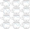 |
Fig. A.1. Accuracy of the spectral calibration by fitting the telluric features in the GRAVITY spectra for each of our epoch measurements for AK For. |
Appendix B: Relative astrometric position of the secondary determined from VLTI/GRAVITY
Relative astrometric position of the secondary component for all systems.
Appendix C: Radial velocities determined from our VLT/UVES observations
Measured radial velocities for all stars.
Appendix D: Parameters of the interferometric calibrators used for the GRAVITY observations
Interferometric calibrators used for our GRAVITY observations taken from the SearchCal software.
Appendix E: Isochrones fit
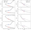 |
Fig. E.1. Fitted PARSEC, BaSTI, MIST, and DSEP isochrones for the HD9312 (left) and HD41255 (right) systems. Luminosities of both components and the radius of the secondary are displayed but not fitted (see text). For HD9312, the black colour is for isochrones with a chosen metallicity of 0.1 dex, while the grey colour is for the metallicity from Kiefer et al. (2018). |
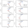 |
Fig. E.2. Fitted PARSEC, BaSTI, MIST, and DSEP isochrones for the HD70937 (left) and HD210763 (right) systems. The black colour is for isochrones with a chosen metallicity of 0.1 dex, while the grey colour is for our measured metallicity. |
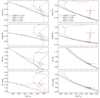 |
Fig. E.3. Fitted PARSEC, BaSTI, MIST, and DSEP isochrones for the HD224974 (left) and HD188088 (right) systems. |
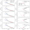 |
Fig. E.4. Fitted PARSEC, BaSTI, MIST, and DSEP isochrones for the LL Aqr (left) and o Leo (right) systems. For LL Aqr, the black colour is for isochrones with a chosen metallicity of 0.15 dex. while the grey colour is for the metallicity from Graczyk et al. (2022). |
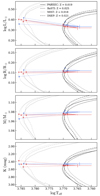 |
Fig. E.5. Fitted PARSEC, BaSTI, MIST, and DSEP isochrones for the V963 Cen system. The black colour is for isochrones with a chosen metallicity of 0.1 ± 0.1 dex, while the grey colour is for the metallicity from Graczyk et al. (2022). |
All Tables
Stellar atmospheric parameters of the hottest component used for the spectral templates to estimate the radial velocities.
Standard deviation of the residuals between the fitted and expected positions of our synthetic companions.
Stellar parameters used for the age determinations, together with our fitted and adopted age for the systems.
Interferometric calibrators used for our GRAVITY observations taken from the SearchCal software.
All Figures
|
Fig. 1. Squared visibility, closure phase, and visibility measurements from the science combiner for AK For observed on 2021 November 8. The data are in blue, while the red dots represent the fitted binary model for this epoch. The residuals (in number of sigma) are also shown in the bottom panels. |
| In the text | |
|
Fig. 2. From top to bottom: combined fit of AK For, HD 9312, and HD 41255. Left: radial velocities of the primary (blue) and the secondary (red) star. Right: GRAVITY astrometric orbit. The shaded grey area represents the 1σ orbit. |
| In the text | |
|
Fig. 3. Same as Fig. 2, but for the system HD 70937, HD 210763, and HD 224974 from top to bottom, respectively. |
| In the text | |
|
Fig. 4. Same as Fig. 2, but for the system HD188088, LL Aqr, and o Leo from top to bottom, respectively. |
| In the text | |
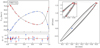 |
Fig. 5. Same as Fig. 2, but for the system V963 Cen. |
| In the text | |
|
Fig. 6. Fitted PARSEC, BaSTI, MIST, and DSEP isochrones for the AK For system. We note that the luminosities were not fitted and were estimated from the Stefan-Boltzmann law. |
| In the text | |
|
Fig. 7. Comparison of the decomposed primary spectrum (blue line) with the synthetic spectrum (red line) for the binary system HD 41255. |
| In the text | |
|
Fig. 8. Comparison of our orbital parallaxes with the Gaia DR3 measurements. |
| In the text | |
|
Fig. 9. Correlations between the RUWE metric, the absolute fractional parallax difference (top), and the photocentre semi-major axis of the systems (bottom). The solid line is the linear correlation law estimated by Stassun & Torres (2021). The dotted vertical line denotes RUWE = 1.4. |
| In the text | |
|
Fig. A.1. Accuracy of the spectral calibration by fitting the telluric features in the GRAVITY spectra for each of our epoch measurements for AK For. |
| In the text | |
|
Fig. E.1. Fitted PARSEC, BaSTI, MIST, and DSEP isochrones for the HD9312 (left) and HD41255 (right) systems. Luminosities of both components and the radius of the secondary are displayed but not fitted (see text). For HD9312, the black colour is for isochrones with a chosen metallicity of 0.1 dex, while the grey colour is for the metallicity from Kiefer et al. (2018). |
| In the text | |
|
Fig. E.2. Fitted PARSEC, BaSTI, MIST, and DSEP isochrones for the HD70937 (left) and HD210763 (right) systems. The black colour is for isochrones with a chosen metallicity of 0.1 dex, while the grey colour is for our measured metallicity. |
| In the text | |
|
Fig. E.3. Fitted PARSEC, BaSTI, MIST, and DSEP isochrones for the HD224974 (left) and HD188088 (right) systems. |
| In the text | |
|
Fig. E.4. Fitted PARSEC, BaSTI, MIST, and DSEP isochrones for the LL Aqr (left) and o Leo (right) systems. For LL Aqr, the black colour is for isochrones with a chosen metallicity of 0.15 dex. while the grey colour is for the metallicity from Graczyk et al. (2022). |
| In the text | |
|
Fig. E.5. Fitted PARSEC, BaSTI, MIST, and DSEP isochrones for the V963 Cen system. The black colour is for isochrones with a chosen metallicity of 0.1 ± 0.1 dex, while the grey colour is for the metallicity from Graczyk et al. (2022). |
| In the text | |
Current usage metrics show cumulative count of Article Views (full-text article views including HTML views, PDF and ePub downloads, according to the available data) and Abstracts Views on Vision4Press platform.
Data correspond to usage on the plateform after 2015. The current usage metrics is available 48-96 hours after online publication and is updated daily on week days.
Initial download of the metrics may take a while.