| Issue |
A&A
Volume 672, April 2023
|
|
|---|---|---|
| Article Number | A76 | |
| Number of page(s) | 18 | |
| Section | Planets and planetary systems | |
| DOI | https://doi.org/10.1051/0004-6361/202244686 | |
| Published online | 04 April 2023 | |
Quasi-simultaneous photometric, polarimetric, and spectral observations of distant comet C/2014 B1 (Schwartz)
1
Astronomical Institute of the Slovak Academy of Sciences, Tatranská Lomnica,
059 60
Vysoké Tatry,
Slovak Republic
e-mail: This email address is being protected from spambots. You need JavaScript enabled to view it.
2
Main Astronomical Observatory of the National Academy of Sciences,
27 Akademika Zabolotnoho St.,
03143
Kyiv,
Ukraine
3
Astronomical Observatory of Taras Shevchenko National University of Kyiv,
3 Observatorna St.,
04053
Kyiv,
Ukraine
4
Institut für Geophysik und Extraterrestrische Physik,
Mendelssohnstraße 3,
38092
TU Braunschweig,
Germany
5
Max Planck Institute for Solar System Research,
Justus-von-Liebig-Weg 3,
37077
Göttingen,
Germany
6
University of Maryland,
College Park, MD
20742,
USA
7
Crimean Astrophysical Observatory,
98409
Nauchny,
Crimea
Received:
5
August
2022
Accepted:
2
February
2023
Abstract
Context. We analyze the results of our comprehensive observations of the high-perihelion comet C/2014 B1 (Schwartz) with stable disk-shaped coma and jets in order to study its nature.
Aims. The main objective of our study is to obtain new observational results for a unique disk-like comet C/2014 B1 (Schwartz) with a perihelion distance of 9.56 au.
Methods. Quasi-simultaneous long-slit spectra, as well as photometric and polarimetric images with g-sdss and r-sdss filters, were acquired with the 6 m telescope of the Special Astrophysical Observatory on 2017 January 23. The BVR-band photometry of the comet was also performed at the 2m telescope of the Peak Terskol Observatory on 2017 January 31. We modeled the dynamics of the jets and the behavior of the color and polarization in the coma considering the dust as aggregated large particles.
Results. We did not reveal any emissions in the spectra. The positions of two jets oriented along the position angles of 179° and 350° and the disk-like shape of the coma have remained unchanged for more than 4 yr. The most realistic model able to explain jets of such stable orientation includes the existence of two active sources located near the north and south poles of the rotating nucleus whose diameter was determined to be between 7.6 and 12.2 km depending on the albedo, of namely between 0.1 and 0.04, respectively. The high activity of the comet is characterized by the high dust production Afρ which varied from 4440 to 3357 cm between 2017 January 23 and 31. A significant difference between the radial surface brightness profiles of the jets and the ambient (undisturbed by the jets) coma is found. The color of the jet structures is much redder than that of the ambient coma, and the nucleus has a very red color, V − R=0.93m±0.19m. There are spatial variations of the color and polarization over the coma and jets.
Conclusions. The observed trends in color and polarization, as well as the brightness profiles, can be explained by the fragmentation of aggregated particles formed by CO2/H2O ices, silicates, and organics, which are of ~1 mm in radius near the nucleus and ~10 μm in radius at the periphery of the coma.
Key words: comets: general / comets: individual: C/2014 B1 (Schwartz) / polarization / scattering / methods: miscellaneous
Deceased.
© The Authors 2023
 Open Access article, published by EDP Sciences, under the terms of the Creative Commons Attribution License (https://creativecommons.org/licenses/by/4.0), which permits unrestricted use, distribution, and reproduction in any medium, provided the original work is properly cited.
This article is published in open access under the Subscribe to Open model. This email address is being protected from spambots. You need JavaScript enabled to view it. to support open access publication.
1 Introduction
The hyperbolic comet C/2014 B1 (Schwartz), hereafter designated C/2014 B1, was discovered on 2014 January 28 by Michael Schwartz at Tenagra Observatory (AZ, USA) using the Tenagra III 0.41m (f/3.75) and 0.81m (f/7) Tenagra II telescopes (Schwartz & Sato 2014). The detected object of about 20m moved at distances of 11.59 and 10.77 au from the Sun and the Earth, respectively, and showed a strongly condensed but slightly elongated coma of 10″–11″ in diameter without an obvious tail. The current orbital elements of the comet are summarized in Table 1 (Reference: JPL 69). The perihelion passage was on 2017 September 10 at a heliocentric distance of 9.56 au, meaning that it is far outside the inner Solar System.
Some characteristics of comet C/2014 B1 were determined by Jewitt et al. (2019) from their observations and modeling. According to these authors, the comet has a coma with a unique disk-like shape and the orientation is stable with respect to the projected anti-solar and orbital directions during the four years after discovery. The comet colors were B − V = 0.85m ± 0.03m and V − R = 0.58m ± 0.03m at the heliocentric distance of 11.88 au. The morphology of the observed coma implies large particles with a mean radius from 0.1 to 10 mm and a dust-mass-production rate of about 10 kg s−1, which is probably sustained by sublimation of volatile ices on the cometary surface. The nucleus radius was estimated to be within the range of 2–20 km (Jewitt et al. 2019). Using his own photometric observations, Paradowski (2020) clarified the size of the cometary nucleus: the effective radius of the nucleus of comet C/2014 B1 was found to be equal to 6.4 ± 0.2 km.
In this paper, we present the results and analysis of comprehensive optical observations of comet C/2014 B1 obtained at a pre-perihelion distance of about 9.6 au. The paper is organized as follows: details of our observations and data reduction are presented in Sect. 2; the results derived from spectroscopy, photometry, and polarimetry are given in Sects. 3–5, and the results of numerical modeling of color, polarization, and brightness profiles are described in Sect. 6. We provide a discussion in Sect. 7, and present our conclusions in Sect. 8.
Selected orbital elements for comet C/2014 B1 (Schwartz).
2 Observations and processing
Spectral, photometric, and polarimetric observations of comet C/2014 B1 were carried out with the 6m Big Telescope Alt-azimuth (BTA) telescope of the Special Astrophysical Observatory (SAO). In addition, the photometric data were derived with the 2m Ritchey-Chretien-Coude (RCC) telescope of the International Center for Astronomical, Medical, and Ecological Research of the National Academy of Sciences of Ukraine located at the Peak Terskol (North Caucasus). Technical information about the telescopes and CCD cameras is presented in Table 2, in which we indicate the telescope, its field of view (FOV), CCD matrix size, image resolution for 1 × 1 binning, pixel scale at the comet distance, filter, and its central wavelength (λ) and full width at half maximum (FWHM).
A summary of observations is given in Table 3. The observation date (the mid-cycle time, UT), the heliocentric (r) and geocentric (∆) distances, the phase angle of the comet (α), the position angle of the scattering plane (ϕ), the filter or grating, the total exposure time (Texp), the number of observation cycles (N), the mode of observations, and the telescope are listed in the table.
2.1 6m BTA telescope
Quasi-simultaneous observations of comet C/2014 B1 were made on 2017 January 23 with the focal reducer SCORPIO-2 (Spectral Camera with Optical Reducer for Photometrical and Interferometrical Observations) attached to the prime focus (f/4) of the 6 m telescope. We used the CCD chip E2V-42-90 with 2K × 4K and 13.5 μm square pixels (see detail Afanasiev & Moiseev 2011; Afanasiev & Amirkhanyan 2012). Photometry and polarimetry of the comet were performed through the Sloan Digital Sky Survey (SDSS) g-sdss (λ4650/1300 Å) and r-sdss (λ6200/1200 Å) broadband filters (see Table 3). To increase the signal-to-noise ratio (S/N), we applied binning of 2 × 2 to the photometric and polarimetric images and 2 × 4 to the spectroscopic frames. For spectral observations, we used the VPHG1200@540 grism and the long slit with dimensions of 6.1arcmin × 1.96arcsec. These provide an effective wavelength region of λ3500–7250 Å (λ4000–7250 Å without strong noise) and a dispersion of 1.62 Å px−1. The spectral resolution is about 10 Å. For absolute calibration, we observed the spectrophotometric standard star BD+33d2642 (Oke 1990). The telescope was tracked on the comet during the exposition. The spectral atmospheric transparency at the SAO was provided by Kartasheva & Chunakova (1978). The twilight morning sky was used for flat-field corrections of the photometric and polarimetric images. To perform wavelength calibration, the spectrum of a He-Ne-Ar lamp was used. To provide flat field corrections for the spectral data, we used a smoothed spectrum of an incandescent lamp. For analysis, we extracted from the rectangular slit image a useful signal from the comet, which corresponds to the flux through the diaphragm, the center of which was located at the comet optocenter and had a diameter of 14.6″ (a projected distance at the comet is 92 304 km). The observation night was photometric with seeing better than 1″.
2.2 2m RCC telescope
Photometric observations of comet C/2014 B1 in the B, V, and R filters were also carried out on 2017 January 31 with the focal reducer attached to the 2m (f/8) telescope of the Peak Terskol Observatory. For observations, we used the CCD imaging detector with 2084 × 2084 pixels and a pixel size of 24 × 24 μm (see Table 2). The image scale was 0.62 arcsec per pixel on the sky and the FOV was about 10.8′ × 10.8′ in 2 × 2 binned mode. To compensate for the motion of the comet during exposures, the telescope was guided at the nonsidereal rate. We obtained a set of exposures from the evening twilight sky through all filters in order to create flat-field images. Absolute flux calibration of the comet images was carried out by measuring field stars. For this, we used the catalogs UCAC4 (Zacharias et al. 2013) and APASS (Henden & Munari 2014). The observations were carried out in conditions with good seeing, of namely ~1.5″.
For all the photometric data, a standard data reduction procedure was followed. A detailed description of the processing of all observational data and the method for calculating polarization parameters with SCORPIO-2 can be found in Afanasiev & Amirkhanyan (2012), Afanasiev et al. (2017), Ivanova et al. (2019, 2021), and with the 2m telescope in Rosenbush et al. (2020).
3 Spectrum of the comet
Cometary spectra include the continuum caused by the scattering of sunlight by dust particles, and molecular emissions. We used a high-resolution solar spectrum (Neckel & Labs 1984) to separate these emissions if they were present in the cometary spectrum. The solar spectrum was transformed to the resolution of the spectrum of comet C/2014 B1 by convolving with the instrumental profile and normalizing to the flux from the comet. The procedure of continuum calculation is described in detail in our previous works (Ivanova et al. 2019, 2021). Figure 1 shows the steps in the calculations of the continuum. Subtracting the calculated continuum from the observed spectrum, we obtained a pure cometary signal. As Fig. 1c displays, no clear emission bands are detected in the emission spectrum. Comparison with the synthetic CO+ spectrum does not show the presence of the CO+ emission in the spectrum of comet C/2014 B1. Previously, ions CO+ and  were detected in comet C/2002 VQ94 (LINEAR) at a distance of 8.36 au from the Sun. This distance is larger than the distances at which ionic emissions were detected in previous objects. In 2009, no emissions were detected from the comet when it was at a distance of 9.86 au (Korsun et al. 2014).
To find the contribution of the gas component to the total flux, we calculated the ratio of the emission component to the total flux through the broadband BVR filters, which is ~3% for the B filter, and about 1.7% for the V and R filters. Using the technique described by Ivanova et al. (2019, 2021), we determined upper limits to the fluxes F of the main cometary emissions and their production rates Q (except for CN because the spectrum in this spectral region is very noisy), although it is very unlikely to detect them in a comet as distant as C/2014 B1 (see Ivanova et al. 2021). To determine fluxes, we used the transmission curves for the C2, C3, and NH2 bands to the spectrum of comet C/2014 B1 (see Table 4). Using the spectral dependence of the reflectivity for the dust, which is determined as the ratio of the comet spectrum Fc(λ) to the scaled solar spectrum Fsun(λ), we found the normalized spectral gradient S′(λ) within the V − R range to be equal to 22.4% ± 2.7% per 1000 Å.
Equipment used for observations.
Log of the observations of comet C/2014 B1 (Schwartz) in 2017 January.
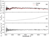 |
Fig. 1 Spectrum of comet C/2014 B1 (Schwartz) derived on 2017 January 23 and its step by step processing. Panel a displays the observed spectrum of the comet (black line) and the scaled spectrum of the Sun (red line) taken from Neckel & Labs (1984), panel b is a polynomial fitting of the ratio of the cometary spectrum to the solar spectrum, and panel c is the residual spectrum, namely the emission spectrum after the cometary spectrum has been subtracted. |
Upper limits for the main molecules in the cometary coma.
4 Results of photometry
4.1 Morphology of the dust coma
All photometric images acquired at the 6m telescope in the g-sdss filter and r-sdss filters were stacked separately for each filter and displayed in Fig. 2, whereas Fig. 3 presents the summed intensity image taken with the 2m telescope in the R filter. As one can see, the disk-like coma is highly asymmetric and elongated in the approximately north–south direction. According to the observations by Jewitt et al. (2019), the shape of the coma of comet C/2014 B1 was morphologically stable within the range of heliocentric distances from 11.8 to 9.6 au.
To reveal the inner structure of the coma and its low-contrast features, we treated the original images with digital filters (see Figs. 2 and 3). Panels b and e show images a and d processed by a rotational gradient method (Larson & Sekanina 1984), whereas panels c and f show images a and d after division by a 1/ρ profile (Samarasinha & Larson 2014). These different enhancement techniques affect the image in different ways. By applying each technique to all individual frames separately, as well as to the same stacking image, and comparing the images, we were able to exclude spurious features (see, e.g., Ivanova et al. 2019, 2021; Picazzio et al. 2019).
Using each image of the comet after digital processing, we determined the position angles (PA) of the jet-like structures. According to the observations on January 23, the position angle of jet J1 is 179° ± 1°, and that of jet J2 is 350° ± 1°. The observations on January 31 are of slightly poorer quality, and so the images in each filter were co-added in order to obtain the position angles of the jets with greater accuracy. Based on our images of the comet and images provided by Jewitt et al. (2019), it can be seen that the disk-like shape of the cometary coma demonstrates unique stability for more than 4 yr.
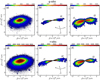 |
Fig. 2 Intensity maps of comet C/2014 B1 (Schwartz) in the g-sdss and r-sdss filters obtained at the 6 m BTA telescope on 2017 January 23. The color scale does not reflect the absolute brightness of the comet. Panels a and d show the co-added composite images of the comet with overlaid isophots differing by a factor of |

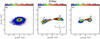 |
Fig. 3 Intensity maps of comet C/2014 B1 (Schwartz) in the R filter obtained with the 2 m RCC telescope on 2017 January 31. The color scale does not reflect the absolute brightness of the comet. Panel a shows the co-added composite image of the comet with the isophots differing by a factor of |

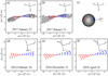 |
Fig. 4 Comparison of the observed images of comet C/2014 B1 (Schwartz) and modeled jets. Panels a and b display the images of the comet taken on 2017 January 23 and on 2017 January 31, respectively, and modeled jets (colored dots): J1 is shown by red circles, and J2 by blue circles. Panel c shows a geometric reconstruction of the viewing conditions of the nucleus which shows how the rotational axis would be seen from the Earth in 2017 January and the location of the north pole PN; the blue circle on the model shows the active area (Source 1) located in the northern hemisphere at the cometocentric latitude +75°, and the red circle is the active area (Source 2) in the southern hemisphere at the latitude −80°. Panels d, e, and f show model jets calculated for images of the comet derived by Jewitt et al. (2019) on 2014 February 26, 2016 December 12, and 2018 April 18, respectively. The arrows point in the directions of the Sun (⊙), north (N), east (E), and the negative projected heliocentric velocity vector of the comet (−V). The negative distance is in the solar direction, and the positive distance is in the anti-solar direction. |
4.2 Active sources on the nucleus
To explain the jet structures revealed in the coma of comet C/2014 B1, we used the geometric model of the origin of jets developed by V. Kleshchonok (see details in Rosenbush et al. 2020; Ivanova et al. 2021). The model takes into account the parameters of the cometary nucleus rotation and the relative position of the Sun, Earth, and comet. For simplicity, we assume that the release of gas and dust occurs with a constant velocity only from the active areas and only when they are illuminated by the Sun. The dispersion of velocities and the acceleration of particles are not taken into account. The model jets are projected on the sky plane.
Figure 4 shows the results of the jet simulation and their correspondence to observations. Assuming that the disk-shaped coma of the comet in the images derived by Jewitt et al. (2019) on 2014 February 26, 2016 December 12, and 2018 April 18 was also formed by two jets, we calculated model jets; these are shown in panels d, e, and f, respectively. As one can see, the model accurately describes the location of the jets and their stable shape over the long period of observations of comet C/2014 B1. The behavior of the jets can be explained by the presence of two active areas on the near-polar surface of the rotating nucleus.
The simulation results, namely, the coordinates of the north pole of the nucleus rotation axis and the cometocentric latitudes of the active areas on the surface of the nucleus are given in Table 5. Both sets of parameters reproduce the picture of jets and differ only in the direction of the nucleus rotation as seen from the Earth. Unfortunately, the location of the axis of rotation does not allow us to determine the speeds of dust in the jets or the rotation period of the nucleus, as any combination of them reproduces the observed picture.
The direction of rotation of the nucleus was determined from comparison of the regions in the unperturbed coma located on diametrically opposite sides of the rotation axis of the nucleus. This comparison can be made using our digital filter, which we refer to as an axial asymmetry filter. If the material is ejected from a colder region after leaving the shadow, then its intensity should be noticeably lower than that from the heated region before entering the shadow. The model image is calculated from the observed image of comet C/2014 B1 using the following expression:
 (1)
(1)
where If is the filtered image, I is the initial brightness distribution in the cometary coma, ρ is the distance from the nucleus, and ϕ is the angle between the divided axis and the radiusvector of the specific image pixel, the length of which is ρ. We considered two cases for such an axis: (i) the position of the axis of rotation of the cometary nucleus is known, and therefore the separation axis is a projection of the axis of the nucleus rotation onto the celestial sphere; or (ii) alternatively, when the position of the rotation axis of the nucleus is unknown then it is possible to choose the Sun–comet direction as the dividing axis.
The result of applying the axial asymmetry filter is presented in Fig. 5, which clearly shows the presence of a significant brightness asymmetry between either side of the dividing axis (the axis of rotation of the comet nucleus). The gray area on the left shows that this region of the nucleus is just starting to heat up, while the white area is already completely illuminated by the Sun. This brightness asymmetry is caused by thermal inertia due to the rotation of the nucleus in the field of the solar radiation. In addition to the axial asymmetry of brightness, a darker northern hemisphere of the coma is observed due to the position of the rotation axis relative to the Sun. Thus, the direction of rotation of the nucleus occurs from east to west on the sky plane. This means that the orientation of the rotation axis of the nucleus of comet C/2014 В1 corresponds to the first set of parameters presented in Table 5.
Table 6 contains the position angles of the northern and southern jets, PA(U) and PA(J2), respectively, measured in our work and those of the northern and southern “arms” of the coma measured by Jewitt et al. (2019). There are also the position angles of the model jets J1 and J2, which were determined using the geometric model with parameters taken from Table 6 for dates covering the entire interval of observations of the comet. An error in the position angle of the model jet is the sum of the errors in the declination of the north pole of the cometary nucleus and in the latitude of the active area that forms the jet. Table 6 also contains the absolute difference between the position angles of the two jets. Comparison of the observed position angles of the northern and southern jets with the position angles of the model jets J1 and J2 shows that they are very close. As in our case the jets are revealed by the rotational gradient method, we can assume that the derived difference between position angles of jets J1 and J2 is real and these jets are not located along the same line, that is, the jets have a slight curvature, as seen in Figs. 2 and 3.
According to Jewitt et al. (2019), there are three alternative models to explain the appearance and location of the observed jets. The first model assumes that the active sources are located on the nucleus near the equator and form a disk of ejected matter that is visible edge-on. According to the second model, two active diametrically opposite active sources are located near the north and south poles of the nucleus, forming two independent jets. In this case, the nucleus rotation axis has a small angle with the sky plane and passes through these jets. The third Lorentz Force Model is rejected by the authors themselves, and so we do not consider it. The first model cannot explain the stability of the morphological structure of the coma for the entire period of observations, which is longer than 4 yr according to Jewitt et al. (2019) This statement is illustrated by Fig. 6, which shows the projections of the orbits of the Earth, Jupiter, Saturn, and comet C/2014 В1 onto the ecliptic plane. The positions of the Earth and the comet are shown for the first and last date of the Jewitt et al. (2019) observations, as well as the date of our observation and the perihelion passage of the comet. During this time, the comet passed an arc in its orbit of larger than 60°, although the Sun–comet–observer angle (i.e., phase angle of the comet) did not change significantly and was within the range from 1.5° to 5.8°. If the position of the axis of the nucleus rotation remains unchanged, then we must certainly observe the variations in the shape of the coma and the direction of the northern and southern “arms” of the coma due to the change in the disk orientation with respect to the observer. Also, due to the low velocity of particle ejection, we should observe the curvature of these arms with the distance from the nucleus because of the acceleration of particles by solar radiation. In reality, the arms remain straight, as indicated by Jewitt et al. (2019) and our data.
Our geometric model confirms the second model and shows the inalterability of the appearance and position of the jets, as shown in Fig. 6. If the axis of rotation is perpendicular to the axis exhibited in the figure (perpendicular to the direction of the jets), then the part of the coma facing the Sun should be brighter. Indeed, the part of the nucleus facing the Sun should heat up to a greater extent, and the polar regions should be constantly illuminated. In reality, we observe the opposite picture, that is, the brighter part of the coma is below the axis in Fig. 5. Therefore, the existence of nearly linear jets with a stable orientation in the coma of comet C/2014 В1 can be explained by the fact that the rotation axis of the nucleus is almost perpendicular to the sky plane, and the active areas are located in the diametrically opposite near-polar areas.
Coordinates of the north rotation pole and the cometocentric latitudes of the active areas on the nucleus of comet C/2014 B1 (Schwartz).
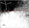 |
Fig. 5 Model image derived after applying the digital axial asymmetry filter to the observed image of comet C/2014 B1 (Schwartz) on 2017 January 31. The position of the nucleus is indicated by a cross, and the red line corresponds to the position of the rotation axis. There is a brightness asymmetry, indicating that the direction of rotation of the nucleus occurs from east to west on the sky plane. |
Position angles of the observed and model jets.
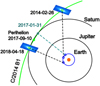 |
Fig. 6 Schematic view of the comet C/2014 B1 (Schwartz) orbit (green line) together with the orbits of Earth, Jupiter, and Saturn for the entire period of observations, including the observations by Jewitt et al. (2019). The position of the comet on the date of our observations is highlighted in turquoise, and the first and last dates of the observations by Jewitt et al. (2019) by the blue rectangle. The moment of the perihelion passage is also marked. |
4.3 Contribution of the nucleus brightness to the coma
In the near-nucleus coma, the integral brightness of a comet is the sum of the coma and the nucleus brightness. To isolate the contribution of the nucleus from this total intensity, it is necessary to separate the contributions of the nucleus and the coma. For this, the theoretical models of brightness distribution in the near-nucleus area of the coma Icoma (excluding the nucleus) and the nucleus Inucl are used. Inucl can be modeled as a point source of light in the form of the two-dimensional Dirac delta function. For the model of the distribution of brightness Icoma across the coma, we followed the methodology employed by Lamy et al. (2011):
 (2)
(2)
However, as Ivanova et al. (2021) showed, it is sometimes necessary to use different exponents n for the radial profiles of the surface brightness from diametrically opposite sides of the nucleus. Such a necessity can be created by various factors, such as when there is inhomogeneity of the nucleus surface or a certain topography and temperature distribution on the cometary nucleus. In general, the observed brightness profile of the comet is compared with the averaged brightness profile of field stars, which is a proxy for the point spread function (PSF) of the telescope. The theoretical brightness profile of the comet I can then be represented by a two-dimensional convolution:
 (3)
(3)
where ⊗ is the convolution operator. Figure 7 demonstrates the normalized radial profiles of the surface brightness of the coma along the solar–anti-solar direction and the averaged brightness profile of field stars (PSF) in the g-sdss and r-sdss filters for the observation on 2017 January 23. Here, we see a noticeable difference between the profile of the coma intensity and the star profile at distances from approximately 5000 km in the solar direction in the g-sdss filter. On short distance scales, it is difficult to investigate near-nucleus phenomena from the ground-based observations. According to Sierks et al. (2015), the brightness profiles change only slightly at small distances from the nucleus. Nonetheless, the contribution of the nucleus brightness changes the brightness gradient in the nearby coma.
For comparison of the theoretical brightness profile of the comet in different directions with the observed surface brightness profiles, it is necessary to take into account a possible distortion of the profiles after stacking images with a random shift of the position of the comet’s optocenter within one pixel. A possible solution to this problem is presented in Appendix A.
We have chosen the least-squares criterion for finding the best solution of Eq. (3), minimizing the sum of the residuals between the modeled and observed profiles at the distances up to ~25 000 km from the nucleus. For the central parts of the coma, which were used to determine the contribution of the nucleus, the S/N was about 100. Table 7 presents the calculation results for the observation of the comet on 2017 January 23, namely: the position angle of profile PA; the power exponents n− for solar direction and n+ for antisolar direction; the contribution of flux from the cometary nucleus to the intensity f0 of the central pixel; the fraction of the central pixel in the total brightness of the nucleus fn; the fraction of the nucleus flux in the integral intensity of the near-nucleus coma within a circular aperture of 5000 km in radius, fn(5000); and the relative error (obs-model), that is, the root mean square (RMS) error of the difference between the observed and modeled brightness distribution. To improve the accuracy of determining the slope (gradient) of the brightness profiles, we additionally calculated several cuts in the coma in the directions with the position angles PA = 53°, 113°, 233°, and 293°. All cuts in the unperturbed coma were found to show the same results within the limits of accuracy. Therefore, in the table we present only the results for cuts along the jets and perpendicular to them. Figure 7 and Table 7 allow us to draw the following conclusions: compared with the star brightness profile, the profiles of the surface brightness of the coma and jets in the r-sdss filter show a significantly greater flux excess in both the inner and outer regions; the profiles in the coma are steeper than in the jets; the coma profiles are steeper in the g-sdss filter; the brightness profiles of the undisturbed coma in the solar direction coincide at the level of measurement accuracy, while there is a significant difference in the slopes in the anti-solar direction; there is no such distinction in the jet profiles.
Figure 8 shows the observed and simulated brightness profiles for the nucleus, coma, and combined nucleus plus coma for the g-ssds and r-ssds images along the selected directions. The profiles of the surface brightness were measured through the central pixel with maximum intensity and the coma perpendicular to the J1-J2 direction (panels a) and along both jets (panels b). The angle between the jets slightly deviates from 180° (171° for our observations, Table 6), but at a distance of 10–15 pixels from the optocenter, this deviation can be neglected. Modeling of the spatial brightness profiles along these directions provides approximately the same values of the contribution of the nucleus to the total intensity of the central pixel. All profiles show a very small contribution of the nucleus brightness to the total brightness of the central part of the coma for the g-ssds filter and a slightly larger contribution for the r-ssds filter. For example, the nucleus contribution to the comet flux within a circular aperture of 5000 km in radius is about two times higher in the r-sdss filter (on average 0.122 ± 0.008) than in the g-ssds filter (on average 0.053 ± 0.007). The nucleus magnitude is therefore ~3.2m (g-sdss) and ~2.4m (r-sdss) fainter than the integral magnitude of the selected near-nucleus area of the coma.
All profiles have exponents n smaller than 1. Such values are typical for the case when the dust characteristics (albedo and scattering cross-section) change rapidly with distance, or when the dust particles return to the near-nucleus coma. For profiles passing through jets, in both filters, n is within 0.5–0.6, while for the profiles in the coma n is within 0.7–0.8, indicating the different evolutionary processes of the dust in the jets and in the coma after the dust is ejected from the cometary nucleus in the near-nucleus region.
Model parameters for different profiles of the surface brightness in the g-sdss and r-sdss filters.
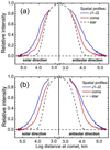 |
Fig. 7 Comparison of the normalized profiles of the surface brightness of comet C/2014 B1 (Schwartz) with the averaged brightness profile of field stars (black dashed line) measured in the g-sdss (a) and r-sdss (b) images on 2017 January 23. The observed profiles were measured through the central pixel with maximum intensity and the coma perpendicular to the J1-J2 direction: PA = 89° for the solar direction and PA = 269° for the anti-solar direction (red solid line) and along both jets in the directions PA(J1)= 179° and PA(J2) = 350° (blue solid line). |
Power index n in the dependence I ∝ ρ−n measured in the g-sdss and r-sdss images of comet C/2014 В1 (Schwartz).
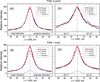 |
Fig. 8 Observed and modeled profiles of the surface brightness of comet C/2014 B1 (Schwartz) in the g-sdss and r-sdss filters along the jets and perpendicular to them for images derived on 2017 January 23. The observed profiles were measured through the central pixel with maximum intensity and the coma perpendicular to the J1-J2 direction (panels a): PA = 89° for the solar direction and PA = 269° for the anti-solar direction and along both jets (panels b) in the directions PA(J1) = 179° and PA(J2) = 350°. The observed and modeled profiles are designated by the black line and colored lines, respectively. The calculated total coma + nucleus profile is shown by a red line; a dashed blue line is the coma profile without the nucleus; and a solid gray line is the nucleus profile. The negative distance is in the solar direction, and the positive distance is in the anti-solar direction. |
4.4 Radial profiles of surface brightness
In the present work, the radial profiles of surface brightness in the g-sdss and r-sdss images are obtained for specific directions, namely for each jet structure J1 and J2 and for the ambient coma in the diametrically opposite directions perpendicular to the J1–J2 direction (Fig. 9). The brightness of the sky background was determined from the mean of the pixels in the region outside the comet without the influence of the brightness of the coma. We estimated the 1−σ brightness uncertainty as ±0.9−1% of the mean. As shown in the figures, there is a significant difference between the intensity profiles in the jets and the coma, but a small distinction between the intensities of the jets in different filters, and almost complete coincidence of the profiles, within the measurement errors, in the solar and anti-solar directions of the coma. The brightness profiles of the undisturbed coma are steeper than those of the jets, and their projected length is limited to ~50 000 km by the brightness of the background sky. The flatter brightness profiles of the jets extend much farther from the nucleus, to a distance of ~ 100 000 km, which may indicate a higher velocity of dust particles in the jets.
Table 8 presents the best-fit parameters of the radial profiles of the surface brightness of comet C/2014 В1 in different directions through the coma and jets in the g-sdss and r-sdss filters for the range of cometocentric distances of approximately 7000–30 300 km for the coma and 6800–79 300 km for the jets. Figure 9 and Table 8 allow us to draw the following conclusions: (i) jet J1 is slightly brighter than jet J2; (ii) there are no significant differences between the slopes in the g-sdss and r-sdss filters for both the coma and the jets, which may indicate a very small contribution of the gas component to the coma of comet C/2014 B1; (iii) the brightness profiles of the undisturbed coma are quite steep (on average n = −1.29); and (iv) three regions with different slopes are clearly distinguished in the brightness profiles of both jets: closer to the nucleus, approximately at cometocentric distances of 7000–25 000 km, n = −0.74; at distances of 25 000–46 000 km, on average n = −1.06, which is very close to the slope of brightness profile of the stationary coma; and finally, at distances of about 45 000–79 000 km the slope is equal to n = −1.36, which is close to that for the undisturbed coma. We see qualitative agreement when comparing the slopes obtained from observations (Table 8) with those from model for the near-nuclear region up to 10 000 km (Table 7).
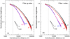 |
Fig. 9 Observed radial profiles of the surface brightness of comet C/2014 B1 (Schwartz) in log–log representation obtained from the calibrated images in the g-sdss (a) and r-sdss (b) bands. The individual curves are cross-cuts measured from the photometric center of the comet through the coma along the jets J1 (black-color) and J2 (red-color), and through the coma in the perpendicular direction to the jets: along the solar direction (PA = 89°, blue) and anti-solar direction (PA = 269°, pink). The near-nucleus area, which may be affected by seeing (1″ which corresponds to 6322 km at the comet), and is delimited here by the vertical dashed line, was not considered. |
Spectrophotometric characteristics of comet C/2014 B1 (Schwartz) observed in 2017 January.
4.5 Color and diameter of the nucleus
Using the magnitudes of the stars in the FOV and the results shown in Table 7, we determined the magnitudes of the nucleus in both filters. The magnitude of the cometary nucleus in the g-ssds filter is 24.18m ± 0.16m, and in the r-ssds filter it is 22.77m ± 0.07m. Consequently, the color index of the nucleus is g−r = 1.41m ± 0.23m. A similarly large value of the color index for the nucleus was found for another distant comet C/2011 KP36 (Spacewatch) of namely g−r = 1.36m ± 0.30m (Ivanova et al. 2021). To convert the Sloan system magnitude to the JohnsonCousins one, we used the transformation coefficients from Jester et al. (2005) for the V filter and from Lupton et al. (2005) for the R filter. As a result, we derived the magnitude of the nucleus in both filters: mV = 23.32m ± 0.11m and mR = 22.39m ± 0.11m and accordingly, V − R = 0.93m ± 0.19m. The absolute magnitude of the nucleus in the V filter of the Johnson-Cousins system is HV =13.70m ± 0.11m.
The absolute magnitude of the comet HV in the V filter was used to estimate the diameter of the nucleus of comet C/2014 B1. Pravec & Harris (2007) provide an expression to calculate the nucleus diameter D:
 (4)
(4)
where pV is the geometric albedo of the nucleus. The range of the geometric albedo is 0.04–0.1, and the diameter of the C/2014 B1 nucleus varies from 12.0 ± 0.3 km to 7.6 ± 0.2 km, respectively, which is within the range of 2–20 km evaluated by Jewitt et al. (2019) and close to the nucleus radius (6.4 ± 0.2 km) defined by Paradowski (2020).
4.6 Observed properties of the dust
To derive the dust characteristics and its production rate, we used the photometric images of comet C/2014 B1 obtained in the g-sdss and r-sdss filters on 2017 January 23 and in the B, V, and R filters on January 31. First of all, we calculated the integral magnitudes from these images. To compare the results for both dates, the magnitudes obtained on January 23 in the Sloan system (g-sdss and r-sdss) were transformed to the Johnson-Cousins system (V and R) using relations determined by Lupton et al. (2005). The apparent magnitudes were measured within the 6″ circular aperture centered on the optocenter, which corresponds to the projected radius of 37 932 km at the comet. The obtained magnitudes of the comet were used to determine the Afρ parameter, which characterizes the dust-production rate of a comet (A’Hearn et al. 1984) and the normalized gradient of reflectivity according to Jewitt & Meech (1987). The results are given in Table 9. Although the comet was at a relatively large heliocentric distance of about 9.6 au, the Afρ values indicate its high activity, which changed significantly between the dates of our observations on January 23 and 31. The reddening S′ in Table 9 obtained from our photometric and spectral observations are close to the average value typical of most distant comets (Storrs et al. 1992; Korsun et al. 2016; Kulyk et al. 2018; Ivanova et al. 2019, 2021). According to Storrs et al. (1992), the mean value of about 22% per 1000 Å was found within the group of 18 ecliptic comets with minimum and maximum values of 15% per 1000 Å and 37% per 1000 Å, respectively.
The dust colors in comet C/2014 B1 obtained from the observations performed on January 23, namely V − R = 0.58m ± 0.05m, and on January 31, namely B − V = 0.85m ± 0.05m and V − R = 0.54m ± 0.05m, are very close to those determined by Jewitt et al. (2019) for this comet. The colors are slightly redder than that of the Sun (B − V = 0.64m ± 0.02m, V − R = 0.35m ± 0.01m; Holmberg et al. 2006), and are redder than the average colors of a number of long-period comets (B − V = 0.78m ± 0.02m, V − R = 0.47m ± 0.02m, see Jewitt 2015). This may indicate that there is a lack of optically small (blue) grains in the near-nucleus area of the coma of comet C/2014 B1.
5 Distribution of color and polarization over the coma
Using the photometric observations of comet C/2014 B1 and the technique described by Ivanova et al. (2019, 2021), we created the g−r color map (Fig. 10a) in order to analyze the dust properties in the coma and in the detected jets. An average error in the magnitude measurements is 0.02m. From the color map, one can see that the near-nucleus area of the comet (up to ~ 10 000 km) has a very red color of ~0.7m on average.
In general, the color of the coma becomes bluer with increasing distance from the nucleus, suggesting evolution of the dust particles. The jet structures are revealed in the color map: the red color of the dust is observed along these structures. The color of the dust within the jets J1 and J2 differ from the color of the coma in the direction of the Sun and in the opposite direction.
The spatial distribution of the degree of linear polarization over the coma in the r-sdss filter is shown in Fig. 10b. The polarization map is shown with isophots superimposed on the image to be able to detect the jets. The red color shows areas with a high degree of polarization, while the blue color presents a low polarization degree (in absolute values). In all areas of the coma, the polarization degree is negative, which means that the plane of polarization is parallel to the scattering plane. A region of low negative polarization is observed in the innermost coma, approximately −1.5% up to distances of about 15 000 km. The figure shows that the polarization gradually increases (in absolute value) from the optocenter to the periphery in all directions (to ~−6%). Isophots show small protrusions in the direction of the jet.
To investigate whether there are any trends in the distribution of color and polarization over the coma, we have taken the radial cross-cuts from the photometric center of the comet along the jets and perpendicular to them (Fig. 11). For this, we measured color and polarization within the coma area of 3 ×3 px2. A comparison of the color and polarization maps in Fig. 11 shows that there is a relation between the changes in color and polarization degree: the color index decreases, while the polarization degree increases (in absolute value) with cometocentric distance. According to Fig. 11 (top panel), the color of the dust drops over a distance of about 120 000 km from the optocenter, from ~0.7m to about ~0.35m, depending on the direction of the cut. The dust in both jets is redder than that in the coma in both directions, although it is significantly redder in the solar directions. The linear polarization in all directions increases (in absolute value) from ~1% to ~6.6%, but this increase is more gradual in the jets than in the coma (Fig. 11, bottom panel). According to our measurements, the degree of polarization integrated within a circular aperture centered on the optocenter with a projected radius of 15 000 km, 45 000 km, and 90 000 km is −1.32 ± 0.12%, −3.27 ± 0.21%, and −5.06 ± 0.34%, respectively, that is, the polarization increases monotonically with distance from the nucleus.
A map of the polarization vectors in the coma presented by the position angles of the polarization plane is shown in Fig. 12. The polarization angles are measured within the coma area of 3 × 3 px2. The orientation of the vectors indicates the direction of the local polarization plane, and their length indicates the degree of polarization. In general, the polarization vectors were found to be practically parallel to the scattering plane. The mean value of the position angles in the coma is about 141° ± 5°, and the polarization plane is parallel to the scattering plane (the position angle of the scattering plane φ = 323.8°); although Fig. 12 demonstrates some deviations, reaching 2°−3°, but these are within the limits of the 1er uncertainty.
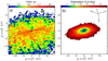 |
Fig. 10 g−r color map (a) and polarization map in the r-sdss filter (b) of comet C/2014 B1 (Schwartz) observed on 2017 January 23 at the phase angle of 2.12°. The polarization map is shown with isophots superimposed on the image to show the polarization in jets. The associated scale bars in magnitude for the color map and in percentage for the polarization map are displayed on the top of the images. The location of the optocenter is marked with a black cross, and jets are shown with black lines. The arrows point in the directions of the Sun (⊙), north (N), east (E), and the negative projected heliocentric velocity vector of the comet (−V). The negative distance is in the solar direction, and the positive distance is in the anti-solar direction. |
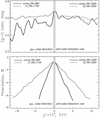 |
Fig. 11 Radial profiles across the g−r color (top panel) and polarization (bottom panel) maps of comet C/2014 B1 (Schwartz). The individual curves are scans measured from the photometric center of the comet through J1 and J2, and the coma in different directions: the solid black line is the cuts along the coma in the directions with PA = 89° and PA = 269°, and the dotted line is the cuts along J1 and J2. Vertical dashed lines show the size of the seeing disk during the observations. The negative distance is in the solar direction, and the positive distance is in the anti-solar direction. |
6 Characteristics of the coma dust particles from the numerical modeling
The observational results reported in the previous sections provide a great opportunity to reveal the properties of the dust particles in comet C/2014 В1. It is well known that polarization and color, being ratios of brightness, depend only on the intrinsic properties of the dust particles and do not reflect the number density variations in the coma as the brightness does, excluding cases of multiple scattering in the optically dense near-nucleus area of the coma. In addition, the spectrum of the comet, which is shown in Fig. 1, is very much featureless, indicating that the color and polarization are defined to a great extent by the dust with negligible gas contamination.
First, we tried to model the dust properties using a model of porous, rough spheroids, which we successfully used to interpret the data for other distant comets (Ivanova et al. 2019, 2021). However, surveying our database of the rough spheroid properties1, we could not find any combination of particle size and composition that, at a phase angle of ~2°, produces a polarization as negative as −6.5% together with the values of the color of the dust coma down to 0.3m (see Fig. 11). Working with the rough spheroid model, we noticed that the polarization becomes more negative as the size of the particles increases. This led to a suggestion that the size of the particles in comet C/2014 B1 exceeds the limits of our database (~ 20 μm), and we turned to the theoretical models that consider light scattering by large dust particles.
The most successful approach to modeling light scattering by large cometary particles was presented by Markkanen et al. (2018) and Markkanen & Agarwal (2019). Here, we used a related approach, where the aggregated large particles are modeled using an extended version of the radiative transfer and coherent backscattering (RT–CB) code (Muinonen 2004) with a static structure factor correction to account for particle aggregation (Cartigny et al. 1986). Following this approach, we considered cometary dust particles as aggregates (agglomerates) of radius rp and stickiness parameter v. Introducing the stickiness parameter to the model allowed us to account for correlated monomer positions and the resulting interference effects by using the Percus-Yevick correlation function for hard sticky spheres (Baxter 1968). We considered a stickiness parameter of v = 0.1, ensuring the monomers in the aggregates are connected, and a variety of particle radii from 5 to 1280 μm.
Our modeling computations revealed some regularities in the light-scattering results that allowed us to narrow down the modeling parameters. We find that, without ice, it is impossible to reproduce a deep polarization minimum, and a red material (organics, silicates) was needed to reproduce the observed color. Also, particles of high porosity were needed to reproduce the observed color and polarization. Based on those findings, the monomers were presented as core-mantle submicron spheres with the core composed of a mixture of silicates (50%) and organics (50%) and the mantle is a mixture of water ice (90%) and CO2 ice (10%). The refractive indexes for the particle materials were taken from Scott & Duley (1996) for silicates, Li & Greenberg (1997) for organics, Warren (1984) for water ice, and Warren (1986) for CO2 ice. The Maxwell-Garnett rule was applied to calculate the effective refractive indices for the core and the mantle. The thickness of the core was assumed to be equal to the thickness of the mantle. The phase curves of polarization for particles of different radii, rp, and two porosities are presented in Fig. 13.
One can see that, at a phase angle of 2°, polarization approaches −8% for particles of rp = 20 μm and porosity 0.975 and at porosity 0.9875 may even exceed −8% for particles of rp = 40 μm at smaller phase angles. We highlight two interesting results seen in Fig. 13. First, the location of the minimum of polarization shifts towards smaller phase angles as the size of particles increases. Second, increasing porosity increases the polarization minimum value and shifts the polarization minimum toward smaller phase angles. Both these effects demonstrate that the model correctly accounts for coherent backscattering as the angular width of the coherent backscattering effect is inversely proportional to the transport mean free path (van der Mark et al. 1988), and thus the effect of coherent backscattering becomes more pronounced for smaller phase angles as particles become larger and/or more porous. For small particles, the transport free path is limited by the particle size as photons can escape from inside the particle in all directions. This explains the strong size dependence. For particles much larger than the transport mean free path, polarization becomes independent of the size. We also note that decreasing particle size first increases and then decreases the polarization minimum value, which is a behavior similar to that observed for comet 67P/Churyumov–Gerasimenko, and for this latter comet was attributed to particle fragmentation, that is, decreasing particle size (Rosenbush et al. 2017).
Figure 14 shows the dependence of polarization and color on particle radius at a phase angle of 2° for particles of two porosities, namely 0.975 and 0.9875, and three radii of monomers (0.16, 0.17, and 0.18 μm). We can see there that the observed combination of color (0.65m) and polarization (~−1%) observed for the near-nucleus area can be reached only for large particles (about 1 mm) of a porosity of 0.9875. The combination of color (~0.5m) and polarization (~−6%) observed at the distance of ~50 000 km from the nucleus can be reproduced by particles of about 10–20 μm in radius, and the better fit is provided by particles of a porosity of 0.975 and a monomer radius of 0.17 μm. All modeled particles reproduce the observed trends: the polarization becomes less negative and the color less red as the size of the particles decreases. Therefore, the modeling provides clear evidence of fragmentation of the particles as they move out of the nucleus, from millimeter (mm)-sized particles near the nucleus to tens of micron sizes at distances of about 100 000 km. We note that the lower porosity that provides a better fit for large distances is consistent with particle fragmentation, as cometary particles have a hierarchical structure (Mannel et al. 2019) where smaller clusters of monomers are more compact than the clusters that form the next level of hierarchy.
We also checked whether or not the discovered characteristics of the dust particles and the idea of their fragmentation are consistent with the change of the surface brightness profile, that is whether or not they can reproduce the trends shown in Fig. 9 and summarized in Table 8. We used the approach described by Jewitt & Meech (1987), presenting the radial surface brightness B as
 (5)
(5)
where K1 is defined by the radius and scattering efficiency of the grains, N is the number density of the dust particles at each point along the line of sight l, and ρ2 = x2−l2 is the projected distance from the nucleus in the sky plane with x defined as the radial distance from the nucleus to a given point on the line of sight. We note that K1 is constant in Jewitt & Meech (1987), whereas it changes in the case of fragmenting particles as particles become smaller. Also, in our case, N changes not only as 1/x2 due to the coma expansion, but also due to particle fragmentation, meaning that the particles have a radius of about 1 mm (more exactly, 1280 μm) at the distance where the first value of polarization and color not affected by seeing were measured (i.e., about x = 6310 km from the nucleus; see Fig. 9) to 10 μm at distances of about x =5×10⁴ km from the nucleus for the coma (see Fig. 11). Particle scattering efficiency was estimated as  , where A is the albedo of the particle of radius rp at a phase angle of 2° as calculated from the aggregate model described above using the albedo definition from Hanner et al. (1981). The computed values of albedo versus particle radius are presented in Fig. 15, where we also represent the data approximation by a polynomial function whose equation is inserted in the figure.
We calculated the particle radius rp as a function of x assuming that the particles changed in radius from 1280 μm to 10 μm so that the radius halved upon every fragmentation. From Fig. 14, it is clear that a constant rate of fragmentation – when large particles and small particles become twice smaller within the same time frame – does not realistically present the change of polarization in comet C/2014 B1, as the change seen from Fig. 11 is linear, whereas Fig. 14 shows almost unchanged polarization for large particles, and then a linear increase in polarization as particles become smaller than ~300 μm. To reproduce the observed trend in polarization, we need to assume that the dust particles quickly disintegrate from mm sizes to sizes of hundreds of microns, probably, within the first 10 000 km, and then the fragmentation slows down so that during the remaining 40 000 km the particle size decreases to 10μm. This is not surprising, as larger aggregates have lower tensile strength than smaller aggregates. Skorov & Blum (2012) found tensile strength T to follow T ≈ fV(rp/1 mm)−2/3, where fV is the volume-filling factor and rp is the aggregate radius. Based on this consideration, we present rp(x) as a function described by two fragmentation rates: a faster one for the first 10 000 km and a slower one for the rest of the observed distances.
Now, in Eq. (5), all variables can be presented as a function of x, which allows easy computation of the brightness B and a comparison of the brightness at two distances, 6310 km and 50 000 km, in order to obtain the value of n = d(log B)/d(log rp), as defined by Jewitt & Meech (1987). With these assumptions, we get a value of n = −1.28, which is close to the values for the coma presented in Table 8. The smaller values of n shown in the table for the jets require slower fragmentation of particles. We obtain n = −1.09 if we assume that particles at a distance of 50 000 km from the nucleus have radii equal to ~60 μm, which allows us to reproduce the polarization of about −3% and a color of slightly below 0.6m (see Fig. 14) typical for the jets as shown in Fig. 11. The slower fragmentation of particles in the jets may result from a different composition or structure of the dust particles or from a larger speed of particles in the jets, transporting particles to larger distances before they fragment significantly.
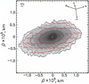 |
Fig. 12 Distribution of the polarization vectors in the coma of comet C/2014 B1 (Schwartz). The map is contoured by isophots superimposed on the image. The orientation of the vectors indicates the direction of the local polarization plane, and the length of the vectors corresponds to the degree of polarization. The arrows point in the directions of the Sun (⊙), north (N), east (E), and the negative projected heliocentric velocity vector of the comet (−V). The negative distance is in the solar direction, and the positive distance is in the anti-solar direction. |
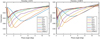 |
Fig. 13 Modeled behavior of polarization at small phase angle depending on the particle radius and porosity. Particles are aggregates of core-mantle monomers of 0.18 μm in radius; the radius of the particles is indicated in the insert. |
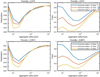 |
Fig. 14 Dependence of polarization and color on the size of particles at a phase angle of 2° for three monomer radii shown in the upper right corner. The top panel shows the results for the porosity of 0.975 and the bottom panel is for the porosity of 0.9875. The insert indicates the radius of the monomers in the aggregates. |
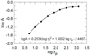 |
Fig. 15 Dependence of the r-sdss albedo of dust particles on their radius. The particles are modeled as aggregates of core-mantle particles as described at the beginning of this section. The albedo values represent an average between those of the particles of porosities of 0.975 and 0.9875. The line shows the polynomial fit to the data, and the equation that describes the best-fit curve is shown at the bottom of the figure. |
7 Discussion
The dynamically new and long-period comets that first entered the inner Solar System from the Oort cloud probably never underwent large temperature changes and may therefore represent the most primitive relics of the proto-solar nebula. Surprisingly, many of these comets are active at very large heliocentric distances (see, e.g., Meech & Svoren 2004; Meech et al. 2009; Kulyk et al. 2018; Farnham et al. 2021) and the mechanisms of this activity are of great interest. We therefore started a long-term program of comprehensive observations of comets (including quasi-simultaneous photometry, polarimetry, and spectroscopy) in order to study their properties at distances where the temperature is too low and water-ice sublimation is negligible, especially comets with large perihelion distances (q > 5 au). To date, only five comets – including comet C/2014 B1 (Schwartz) – with perihelion distances greater than 9.5 au have been observed: three hyperbolic comets – C/2003 A2 (Gleason) (q =11.43 au), C/2000 A1 (Motani) (q = 9.743 au), and C/2014 B1 (Schwartz) (q = 9.557 au); and two near-parabolic comets – C/2014 UN271 (Bernardinelli-Bernstein) (q=10.950au) and C/2010 L3 (Catalina (CSS)) (q = 9.883 au). All these comets demonstrated various levels of physical activity and therefore provide some insight into the nature of the activity in these distant comets. Our estimates of the diameter of the nucleus of the comet C/2014 B1 indicate that it lies within the range of 7.6–12.0 km depending on the albedo used, that is, 0.1–0.04. According to our pre-perihelion measurements, the comet exhibited high activity characterized by large values of Afρ, indicating a high dust-production rate, which significantly varied, from 4440 cm on 2017 January 23 to 3357 cm on January 31. A comparison of the obtained values Afρ with those for a sample of selected nearly isotropic comets highlighted their significantly lower activity at the heliocentric distances from 4.6 to 12.64 au (Kulyk et al. 2018). The primary cause of the diversity in the activity among the observed Oort cloud comets may be the comet formation conditions in the protosolar nebula and the composition and abundance of volatiles in the nucleus (for details, see the review by Biver et al. 2022). When a comet is within the inner Solar System, the main driver of its activity is water ice, the most abundant species among the cometary ices. At large heliocentric distances, of 9.6 au for comet C/2014 B1 for example, the more volatile cometary ices of CO and CO2 sublimate near the surface of the nucleus and are believed to drive the activity in distant comets. According to Biver et al. (2022, and references therein), in some comets, CO sublimation can lift dust into the coma even at distances of more than 20 au from the Sun, whereas in other comets, CO2 can become the major constituent of the coma even at r > 2.5 au, in both cases driving the activity of the comet. It cannot be excluded that crystallization of amorphous water ice may be another trigger of the activity at large heliocentric distances that sustains cometary activity.
In general, the activity of comets beyond the orbit of Jupiter can vary significantly and have long-lasting characteristics. Some distant comets were seen to have extended tails and compact coma (Meech et al. 2009; Korsun et al. 2010; Ivanova et al. 2015, 2019), which is different from the morphology of comets at small heliocentric distances. At the same time, it was found that the activity of some distant comets presented itself as extensive and asymmetrical comae, without the classic tails (Korsun et al. 2016; Ivanova et al. 2021), but with active structures (jets). Similar behavior was exhibited in comet C/2014 B1, demonstrating a strong asymmetry of the coma due to two jets (along the directions with position angles of 179° and 350°) located nearly perpendicular to the sunward direction in the image plane, but there was no regular tail. The disk-like shape of the cometary coma, and, accordingly, the structure of the jets, remained essentially unchanged throughout the entire time the comet was visible, from 2014 until 2021 (this work, Jewitt et al. 2019)2. Our study shows that the formation of a stable disk-shaped coma with fixed orientation, despite the changing observational geometry, can be caused by two diametrically opposite active sources located near the north and south poles of the nucleus, forming two independent jets. Jewitt et al. (2019) also considered the possibility of interpreting the optical appearance of the coma using a model with two jets that emerge from active regions on opposite sides of the nucleus near the sunrise and sunset terminators, but these authors indicated a number of difficulties resulting from this model.
The presence of active structures may be confirmed by radial brightness profiles of distant comets, which have gradients different from n = −1, which is characteristic of a spherically symmetric steady-state coma (Ivanova et al. 2019, 2021). Factors such as gas drag, solar radiation pressure, sublimation and fragmentation of particles, and variable mass loss from the nucleus may be responsible for this deviation (Jewitt & Meech 1987; Farnham 2007). Our study of the distribution of surface brightness along the jet structures and undisturbed coma of comet C/2014 B1 at different distances from the nucleus shows (Fig. 9) that the brightness profiles of the undisturbed coma are significantly steeper than those of the jets and become faint up to distances of about 50 000 km. At the same time, we revealed that both jets may be divided into three distinct regions, in which the slopes are increasing with distance from the nucleus, and the profiles themselves become steeper as ρ increases, reaching a distance of about 100 000 km. The revealed differences between the coma and jet profiles, and between the corresponding gradients, may indicate different particle speeds. It appears that particles are lifted at low speeds from the illuminated region of the nucleus, and that those with higher speeds are released from the active sources on the nucleus, forming the jets. These differences may also indicate changes in the physical properties of the dust itself with increasing cometocentric distance. The processes affecting the properties of dust particles may lead to different results for the unperturbed coma and jets. Our results (Table 8) show that the slope changes along both jets, and in addition that it changes more rapidly at larger cometocentric distances (see also Jewitt et al. 2019). The behavior of the brightness profiles and the absence of a dust tail may indicate the presence of large particles within the near-nucleus coma of comet C/2014 B1, which were ejected from the nucleus more slowly and due to sublimation underwent fragmentation processes in the process of moving away from the nucleus and cannot be significantly affected by solar radiation pressure. Further fragmentation (up to ~50 000 km) can lead to smaller particles and, in the absence of radiation pressure, the establishment of the regime of steady and free-flying particles. Accordingly, the gradient of brightness profiles should be near n = −1. At distances of up to ~80 000 km, even the weak effect of the radiation pressure may accelerate the smaller, fragmented grains and provide n ≈ −1.3, which is exactly the same as for the unperturbed coma.
At large heliocentric distances, the highly volatile ices, most likely CO/CO2 and/or N2, entrain dusty particles forming observed comae and tails. However, so far, the gaseous emissions have only been observed in the optical spectral region for a few distant comets (Korsun et al. 2006, 2008, 2014; Ivanova et al. 2021), while most of the observed spectra at large heliocentric distances are featureless (Rousselot et al. 2014; Womack et al. 2017; Ivanova et al. 2019). As in the majority of distant comets, comet C/2014 B1 did not reveal any gaseous emissions in the visible range of the spectrum; there was only a continuum. The obtained values of reddening (Table 9) are close to the average value typical of most distant comets (Storrs et al. 1992; Korsun et al. 2016; Kulyk et al. 2018; Ivanova et al. 2019, 2021). We find the colors of comet C/2014 B1, namely B − V = 0.85m ± 0.05m and V − R = 0.56m ± 0.05m, which are in very good agreement with the measured colors by Jewitt et al. (2019), to be red in the optical range, which is typical for comets and is consistent with the scattering of solar light by dust. The dust color in the comet did not change during the entire period of observations from 2014 to 2018 (Jewitt et al. 2019). This indicates that the physical and chemical characteristics of the ejected dust were not changing and the level of incessant activity remained the same, ensuring the release of large particles into the coma. The color map of comet C/2014 B1 (Fig. 10) shows that the color of the jet structures is much redder than that of the ambient coma. However, the near-nucleus region of the coma is the reddest (see Figs. 10 and 11), which may be explained by the contribution of a very red nucleus to the color of the nearest coma and/or by large particles (Ivanova et al. 2019, 2021; Kulyk et al. 2021). According to our estimation, the color of the nucleus of comet C/2014 B1, namely of V − R = 0.93m, is much redder than the dust coma. Comet C/2011 KP36 (Spacewatch) also had an ultra-red nucleus, B−R = 1.9m, while the color of the cometary coma was B−R =1.22m; although the measurements of color were made at a much smaller distance from the Sun, of 5.06au (Ivanova et al. 2021). In general, the colors of cometary nuclei (with some contribution of the dust coma) observed at large heliocentric distances (with q > 5.2 au) are redder than the Sun, and these colors range from slightly blue to very red (Jewitt 2015). An unusually red color was measured at the comparable heliocentric distance of r = 8.6 au in the coma of comet 166P/2001 T4 (NEAT) with the perihelion at q = 8.559 au (Bauer et al. 2003; Jewitt 2009; Shi & Ma 2015). On average, the color in the inner coma of 166P, within 9600 km, was very red, namely V − R = 0.95m. However, the red color of this comet does not reflect the color of the nucleus itself, because the measurements were contaminated by the active coma. To date, the colors of most other comets measured at heliocentric distances comparable to or smaller than that of C/2014 B1, but beyond the water-ice sublimation zone, contained substantial coma (see, e.g., Lamy & Toth 2009; Jewitt 2015; Kulyk et al. 2018). As a result, the color of these comets may be dominated by dust particles, not by the central nucleus. According to Jewitt (2015), various colors of the nucleus and the dust coma in the near-nucleus area of a given comet can be caused by intrinsically different colors or by the fact that the properties of the particles change with time following their release from the nucleus. The further evolution of dust with distance from the nucleus is specific to any given comet and depends on the characteristics of both the dust and the comet nucleus itself.
Except for polarimetric observations of comets 29P/Schwassmann-Wachmann at r ≈ 5.9 au (Kochergin et al. 2021) and C/2017 K2 (PANSTARRS) at r ≈ 6.8 au (Zhang et al. 2022), there are no data on the polarization of comets with a perihelion distance beyond the orbit of Jupiter. We measured the linear polarization and created a map of its spatial distribution over the coma of comet C/2014 B1 at the record heliocentric distance of 9.6 au. The polarization of the dust coma of the comet varied from the values typical of comets at a phase angle of 2.1°, ranging from about −1% near the nucleus, to extremely large values of about −6.5% at distances of approximately 105 km from the nucleus. Typical values of the minimum polarization degree at the negative polarization branch for distant comets (within the range 7 > r > 4 au) are much higher (in absolute value; Dlugach et al. 2018; Kochergin et al. 2021; Ivanova et al. 2019, 2021) than the average value (Pmin ~−1.5%) observed for the dust coma of most comets closer to the Sun (Kiselev et al. 2015). A comparison of the color and polarization maps shows that there is an unambiguous relationship between the changes of color and the degree of polarization, which could be the result of changes in the sizes and/or optical properties of the paricles.
A comprehensive set of observational data provided us with an unprecedented opportunity to reveal the physical properties of the pristine dust particles and to study processes in the coma of a distant comet by modeling various observed characteristics and looking for the solutions that consistently reproduce different types of observational data. We carried out computer modeling using an RT-CB approach that includes light-scattering computations for large particles of complex structure. Specifically, we considered aggregated particles formed by core-mantle monomers with a H2O/CO2 mantle and a silicate/organic core. Our modeling revealed that only highly porous mm-sized particles can produce the polarization and color observed near the nucleus, confirming the conclusion of Jewitt et al. (2019) as to the existence of large mm-sized particles in the near-nucleus coma. However, we also reveal that the particles are much smaller far from the nucleus, down to 10 μm, remaining still highly porous but slightly more compact. We also find that the jet particles reach a size of 10μm at much larger distances from the nucleus than are required for the coma particles to reach this size. This is in accordance with our conclusions regarding the higher speed of material in the jets as revealed by our analysis of the brightness profiles. Thus, the modeling not only reveals the composition, structure, and size of the dust particles, but also provides strong evidence supporting the dust fragmentation that appears to be consistent with the observed brightness profile. Our modeling results also allow us to explain the observed differences between the coma and the jets, thus completing the picture of the dust characteristics and processes in the coma.
8 Conclusions
In this paper, we study the unusual, dynamically new comet C/2014 B1 (Schwartz) with a relatively large perihelion (q = 9.56 au). This comet was observed at a heliocentric distance of r = 9.64 au pre-perihelion. C/2014 B1 is particularly interesting because of the disk-like shape of its coma, which remained almost unchanged throughout observations – when the comet was visible – from 2014 until 2021, despite the changing observational geometry.
Images, spectra, radial profiles of surface brightness, a color map, and a polarization map obtained from quasi-simultaneous photometric, spectroscopic, and polarimetric observations with the g-sdss and r-sdss filters at the 6m telescope of the Special Astrophysical Observatory demonstrate the uniqueness of comet C/2014 B1 (Schwartz). The main results of the observations and their interpretation using computer modeling of the dust properties can be summarized as follows:
The activity level measured by the Afρ parameter varied from 3357 ± 110 to 4440 ± 500 cm in the R filter, which implies that C/2014 B1 is a very active comet despite its large perihelion distance. This is probably due to the sublimation of supervolatile ices from the relatively large nucleus, the diameter of which is between 7.6 km and 12.2 km depending on the albedo of between 0.1 and 0.04, respectively;
No gas emissions were detected in the spectrum of comet C/2014 B1 at the heliocentric distance of 9.64 au; there was only continuum caused by the scattering of sunlight by dust particles;
Two strong jet-like structures oriented along the position angles of 179° ± 1° and 350° ± 1° were detected in the coma. Modeling these jet structures shows that the observed unchanging disk-like shape of the coma and the position of the jets during the 4 yr of observations can be explained by the existence of two active sources located near the north and south poles of the rotating nucleus, forming two independent jets, namely J1 at a latitude of +80° and J2 at −75°. We determined the position of the rotation axis of the nucleus (
 ,
,  ) and the direction of its rotation;
We find a significant difference between the radial profiles of the surface brightness of the jets and those of the undisturbed coma. The brightness profiles of the coma are steeper than those of the jets, and become faint at projected distances of larger than 50 000 km, while the flatter brightness profiles of the jets extend much farther from the nucleus, to at least 100 000 km. Three regions with different slopes are clearly distinguished in the brightness profiles of the two jets, namely the slope increases with distance from the nucleus: n = −0.74, −1.06, and −1.36 at appropriate distance ranges of 7000–25 000 km, 25 000–46 000 km, and 45 000–79 000 km, respectively. The slope in the outer region is close to that of the coma, namely n = −1.29;
The color of the cometary dust is redder than the Sun: in 2017, on January 23, V − R = 0.58m ± 0.05m, and on January 31, B − V = 0.85m ± 0.05m and V − R = 0.54m ± 0.05m. The color of the cometary dust was stable throughout the entire observation period from 2014 to 2018. We derived the very red color of the nucleus (V − R = 0.93m ± 0.19m), finding it to be much redder than the color of the dust coma. The color of the jet structures is much redder than in the ambient (undisturbed by the jets) coma. The mean value of the normalized spectral gradient is 22%/1000 Å, which is close to the average value typical of the majority of distant comets;
We detected the spatial variations of the color and polarization over the coma: the g-r color changes from about 0.2m to 0.7m, and the polarization degree varies from about −1% to −6.5% at the phase angle of 2.1°. There is an unambiguous relationship between the changes in the color and the degree of polarization. The near-nucleus region is characterized by a low negative degree of polarization and red color; at the periphery, there is high negative polarization and a slightly bluer color;
Modeling that combines the RT-CB approach with the static structure factor correction reveals that highly porous mm-sized aggregates of ices and some red material (e.g., organics, silicates) can reproduce the near-nucleus polarimetric and color characteristics of comet C/2014 B1. The particles in the outer coma are consistent with 10−20 μm aggregates, indicating fragmentation of particles. The modeling results also allow us to reproduce the observed brightness profiles and explain the difference between them for the jets and the ambient coma;
Comprehensive observations, which included spectral, photometric, colorimetric, and polarimetric imaging observations, combined with a comprehensive modeling accomplished for all observational data types revealed the unique composition, structure, and size of the coma and jet dust particles, providing a consistent picture of the comet materials and processes taking place therein, and demonstrating the power of this comprehensive approach.
Acknowledgements
The authors note the great contribution of Prof. Viktor Afanasiev to this work, who passed away on December 21, 2020. He actively participated in the observations of comet C/2014 B1 (Schwartz) at the 6-m telescope of the Special Astrophysical Observatory with the multi-mode focal reducer SCORPIO-2 which was designed and developed under his leadership. The work by OI and MH was supported by the Slovak Grant Agency for Science VEGA (Grant No. 2/0059/22) and by the Slovak Research and Development Agency under Contract No. APVV-19-0072. The research by OI, VR, IL, VK is supported by Project no. 0122U001911 of the Taras Shevchenko National University of Kyiv. JM is supported by the European Union’s Horizon 2020 research and innovation program under grant agreement no. 757390.
Appendix A Using the Moffat function to correctly determine the point spread function
To correctly determine the contribution of the nucleus brightness to the brightness of the dusty coma, it is necessary to accurately determine the PSF of the comet image. As a rule, images of several stars in the FOV of a comet are used and, accordingly, the average profile is determined from these star images. However, due to the finite size of the pixel, the center of the star image can occupy any position within the spatial dimensions of the pixel. When stellar profiles are superimposed, the centers of which are randomly distributed, the symmetry is distorted, and the average profile is expanded (Fig. A.1). We can see that the center of the star image does not coincide with the center of the pixel (Fig. A.1b) and, as a result, the asymmetry and distortion of the star profile are clearly visible. Therefore, to correctly determine the PSF, it is necessary to take into account the discrepancy between the position of the star center and the pixel center.
To resolve this problem, we propose the following algorithm. We assume that we know the type of theoretical brightness distribution in the star image as a function F(x, y, a1,…, an), where x, y are rectangular coordinates on the image, and are unknown parameters that need to be determined. First, we need to correctly determine the background level near the star. To do this, as an initial approximation of the position of the star center, we choose the coordinates xm, ym, which are the coordinates of the pixel with the maximum intensity in the star image. Then we determine the average value of the pixel intensities and the error of this value in two annular diaphragms with sizes of n < ρ1 ≤ (n + 2) and (n +1) <ρ2 ≤ (n + 3), where ρ is the distance in pixels from the pixel with the maximum intensity of the star. In the process of determining the background, n increases until the difference between the average intensity in each of the two apertures becomes smaller than the error. The radius of the star image in pixels is taken equal to n, and the second annular aperture of a larger diameter is used to determine the background. To take into account the possible dependence of the background on the coordinates, the background level is determined as a linear dependence:
 (A.1)
(A.1)
where b0, bx, and by are determined by the least squares method for annular diaphragms with the size of (n + 1) < ρ2 ≤ (n + 3), x and y are cartethian coordinates in pixels from the pixel with star maximum intensity.
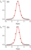 |
Fig. A.1 Comparison of the profiles of the model (solid line) and measured image of the same star (dots) along the X (plot a) and Y (plot b) axes. The profiles are normalized to the maximum value of 1. The profile of the star depends on the center position of the star within one pixel. On the X-axis, the center of the star image coincides with the middle of the pixel, whereas it is slightly shifted on the Y-axis. |
The refined position of the star xc, yc is determined from the distribution of the brightness in the star image I(x, y) after removing the background b(x, y):
 (A.2)
(A.2)
To model the brightness distribution in star image, we use the Moffat function M(x, y) (Moffat 1969):
![Mathematical equation: $M\left( {x,y} \right) = {A \over {\left[ {1 + {\textstyle{{{{\left( {x - {x_c}} \right)}^2} + {{\left( {y - {y_c}} \right)}^2}} \over {\rho _0^2}}}} \right]\beta }},$](/articles/aa/full_html/2023/04/aa44686-22/aa44686-22-eq22.png) (A.3)
(A.3)
where A, β, and ρ0 are parameters of the Moffat function. If the ordinal number of pixels in the star image is k along the X axis and l along the Y axis, then the model brightness of the image in this pixel will be:
 (A.4)
(A.4)
where k and l are number of pixels in star image along the X and Y axes, respectively. Parameters Moffat-functions A, β, and ρ0 are determined using the least squares test of the difference between the entire measured image of the star and the model image. Fig. A.1 shows the profiles of the simulated and measured images of the same star along the X (Fig. A.1a) and Y (Fig. A.1b) axes. The solid line is the model distribution and the dots show the brightness of individual pixels. It can be seen that if the center of the star image coincides with the center of the pixel, then the model and pixels on the star image almost coincide. Otherwise, the profiles are significantly different and the measured profile cannot be used as a real PSF.
In order to maximize the reliability of the results, the profiles of several stars are determined using this method for subsequent averaging. As individual images of stars have a noise component that can affect the determined model parameters, in order to reduce it, when determining the PSF, we take an average of the model profiles of several stars with weights inversely proportional to the approximation errors by the Moffat function. At this stage, it is possible to reject individual profiles due to high noise levels or distortion of the PSF profile. The resulting PSF profile for each frame is used to process images of the comet in the same frame.
References
- Afanasiev, V. L. & Amirkhanyan, V. R. 2012, Astrophys. Bull., 67, 438 [NASA ADS] [CrossRef] [Google Scholar]
- Afanasiev, V. L. & Moiseev, A. V. 2011, Baltic Astron., 20, 363 [NASA ADS] [Google Scholar]
- Afanasiev, V. L, Amirkhanyan, V. R., Moiseev, A. V. et al. 2017, Astrophys. Bull., 72, 458 [NASA ADS] [CrossRef] [Google Scholar]
- A’Hearn, M. F., Schleicher, D. G., Millis, R. L., et al. 1984, AJ, 89, 579 [CrossRef] [Google Scholar]
- Bauer, J. M., Fernández, Y. R., & Meech, K. J. 2003, PASP, 115, 981 [CrossRef] [Google Scholar]
- Bauer, J. M., Grav, T., Blauvelt, E., et al. 2013, ApJ, 773, 22 [Google Scholar]
- Baxter, R.J. 1968, J. Chem. Phys., 49, 2770 [NASA ADS] [CrossRef] [Google Scholar]
- Biver, N., Dello Russo, N., Opitom, C., et al. 2022, ArXiv e-prints [arXiv:2207.04800] [Google Scholar]
- Cartigny, J. D., Yamada, Y., & Tien, C. L. 1986, J. HeatTransf., 108, 608 [CrossRef] [Google Scholar]
- Dlugach, J. M, Ivanova, O. V., Mishchenko, M. I. et al. 2018, JQSRT, 205, 80 [NASA ADS] [CrossRef] [Google Scholar]
- Farnham, T. 2007, DPS, 39, 54.05 [NASA ADS] [Google Scholar]
- Farnham, T. L., Kelley, M. S. P., & Bauer, J. M. 2021, Planet. Sci. J., 2, 236 [NASA ADS] [CrossRef] [Google Scholar]
- Hanner, M. S., Giese, R. H., Weiss, K., et al. 1981, A&A, 104, 42 [NASA ADS] [Google Scholar]
- Henden, A. & Munari, U. 2014, Contrib. Astron. Observ. Skalnate Pleso, 43, 518 [NASA ADS] [Google Scholar]
- Holmberg, J., Flynn, C., & Portinari, L. 2006, MNRAS, 367, 449 [NASA ADS] [CrossRef] [Google Scholar]
- Ivanova, O. V, Dlugach, J. M., Afanasiev, V. L. et al. 2015, Planet. Space Sci., 118, 199 [NASA ADS] [CrossRef] [Google Scholar]
- Ivanova, O., Luk’yanyk, I., Kolokolova, L., et al. 2019, A&A, 626, A26 [NASA ADS] [CrossRef] [EDP Sciences] [Google Scholar]
- Ivanova, O., Rosenbush, V., Luk’yanyk, I., et al. 2021, A&A, 651, A29 [NASA ADS] [CrossRef] [EDP Sciences] [Google Scholar]
- Jester, S., Schneider, D. P., Richards, G. T., et al. 2005, AJ, 130, 873 [Google Scholar]
- Jewitt, D. 2009, AJ, 137, 4296 [Google Scholar]
- Jewitt, D. 2015, AJ, 150, 201 [NASA ADS] [CrossRef] [Google Scholar]
- Jewitt, D., & Meech, K. J. 1986, ApJ, 310, 937 [Google Scholar]
- Jewitt, D. C. & Meech, K. J. 1987, ApJ, 317, 992 [NASA ADS] [CrossRef] [Google Scholar]
- Jewitt, D., Kim, Y., Luu, J. et al. 2019, AJ, 157, 103 [NASA ADS] [CrossRef] [Google Scholar]
- Kartasheva, T. A. & Chunakova, N. M. 1978, Astrofiz. Issledov. Izv. Spetsial’noj Astrofiz. Observ., 10, 44 [Google Scholar]
- Kiselev, N., Rosenbush, V., Levasseur-Regourd, A., & Kolokolova, L. 2015, Comets, in Polarimetry of Stars and Planetary Systems, eds. L. Kolokolova, J. Hough, & A. Levasseur-Regourd (Cambridge: Cambridge University Press), 379 [CrossRef] [Google Scholar]
- Kochergin, A., Zubko, E., Chornaya, E. et al. 2021, Icarus, 366, 114536 [NASA ADS] [CrossRef] [Google Scholar]
- Korsun, P. P., Ivanova, O. V., & Afanasiev, V. L. 2006, A&A, 459, 977 [NASA ADS] [CrossRef] [EDP Sciences] [Google Scholar]
- Korsun, P. P., Ivanova, O. V., & Afanasiev, V. L. 2008, Icarus, 198, 465 [Google Scholar]
- Korsun, P. P, Kulyk, I. V., Ivanova, O. V. et al. 2010, Icarus, 210, 916 [NASA ADS] [CrossRef] [Google Scholar]
- Korsun, P. P., Rousselot, P., Kulyk, I. V., et al. 2014, Icarus, 232, 88 [Google Scholar]
- Korsun, P. P, Ivanova, O. V., Afanasiev, V. L. et al. 2016, Icarus, 266, 88 [NASA ADS] [CrossRef] [Google Scholar]
- Kulyk, I., Rousselot, P., Korsun, P. P., et al. 2018, A&A, 611, A32 [NASA ADS] [CrossRef] [EDP Sciences] [Google Scholar]
- Kulyk, I., Korsun, P., Lukyanyk, I. et al. 2021, Icarus, 355, 114156 [NASA ADS] [CrossRef] [Google Scholar]
- Lamy, P. & Toth, I. 2009, Icarus, 201, 674 [NASA ADS] [CrossRef] [Google Scholar]
- Lamy, P. L., Toth, I., Weaver, H. A., et al. 2011, MNRAS, 412, 1573 [Google Scholar]
- Larson, S. M., & Sekanina, Z. 1984, AJ, 89, 571 [NASA ADS] [CrossRef] [Google Scholar]
- Li, A., & Greenberg, J. M. 1997, A&A, 323, 566 [NASA ADS] [Google Scholar]
- Lupton, R. H., Juric, M., Ivezic, Z., et al. 2005, Bull. Am. Astron. Soc., 37, 1384 [Google Scholar]
- Mannel, T., Bentley, M. S., Boakes, P. D., et al. 2019, A&A, 630, A26 [NASA ADS] [CrossRef] [EDP Sciences] [Google Scholar]
- Markkanen, J., & Agarwal, J. 2019, A&A, 631, A164 [NASA ADS] [CrossRef] [EDP Sciences] [Google Scholar]
- Markkanen, J., Agarwal, J., Väisänen, T. et al. 2018, ApJ, 868, L16 [NASA ADS] [CrossRef] [Google Scholar]
- Meech, K. J., & Svoren, J. 2004, Comets II, eds. M. C. Festou, H. U. Keller, & H. A. Weaver (Tucson: University of Arizona Press), 317 [Google Scholar]
- Meech, K. J., Pittichová, J., Bar-Nun, A., et al. 2009, Icarus, 201, 719 [NASA ADS] [CrossRef] [Google Scholar]
- Moffat, A. F. J. 1969, A&A, 3, 455 [NASA ADS] [Google Scholar]
- Muinonen, K. 2004, Waves in Random Media, 14, 365 [NASA ADS] [CrossRef] [Google Scholar]
- Neckel, H. & Labs, D. 1984, Sol. Phys., 90, 205 [NASA ADS] [CrossRef] [Google Scholar]
- Oke, J.B. 1990, AJ, 99, 1621 [NASA ADS] [CrossRef] [Google Scholar]
- Paradowski, M.L. 2020, MNRAS, 492, 4175 [NASA ADS] [CrossRef] [Google Scholar]
- Picazzio, E., Luk’yanyk, I. V., Ivanova, O. V., et al. 2019, Icarus, 319, 58 [NASA ADS] [CrossRef] [Google Scholar]
- Pravec, P., & Harris, A. W. 2007, Icarus, 190, 250 [CrossRef] [Google Scholar]
- Rosenbush, V. K, Ivanova, O. V., Kiselev, N. N. et al. 2017, MNRAS, 469, S475 [NASA ADS] [CrossRef] [Google Scholar]
- Rosenbush, V., Ivanova, O., Kleshchonok, V. et al. 2020, Icarus, 348, 113767 [Google Scholar]
- Rousselot, P., Korsun, P. P., Kulyk, I. V., et al. 2014, A&A, 571, A73 [NASA ADS] [CrossRef] [EDP Sciences] [Google Scholar]
- Samarasinha, N. H. & Larson, S. M. 2014, Icarus, 239, 168 [NASA ADS] [CrossRef] [Google Scholar]
- Schwartz, M. & Sato, H. 2014, CBET, 3797, 1 [NASA ADS] [Google Scholar]
- Scott, A., & Duley, W.W. 1996, ApJS, 105, 401 [NASA ADS] [CrossRef] [Google Scholar]
- Shi, J. C. & Ma, Y. H. 2015, MNRAS, 454, 3635 [NASA ADS] [CrossRef] [Google Scholar]
- Sierks, H., Barbieri, C., Lamy, P. L., et al. 2015, Science, 347, aaa1044 [Google Scholar]
- Skorov, Y. & Blum, J. 2012, Icarus, 221, 1 [NASA ADS] [CrossRef] [Google Scholar]
- Storrs, A. D., Cochran, A. L., & Barker, E. S. 1992, Icarus, 98, 163 [Google Scholar]
- van der Mark, M. B., van Albada, M. P., & Lagendijk, A. 1988, Phys. Rev. B, 37, 3575 [CrossRef] [Google Scholar]
- Warren, S.G. 1984, Appl. Opt., 23, 1206 [NASA ADS] [CrossRef] [Google Scholar]
- Warren, S.G. 1986, Appl. Opt., 25, 2650 [NASA ADS] [CrossRef] [Google Scholar]
- Womack, M., Sarid, G., & Wierzchos, K. 2017, PASP, 129, 031001 [Google Scholar]
- Zacharias, N., Finch, C. T., Girard, T. M., et al. 2013, AJ, 145, 44 [Google Scholar]
- Zhang, Q., Kolokolova, L., Ye, Q. et al. 2022, Planet. Sci. J., 3, 135 [NASA ADS] [CrossRef] [Google Scholar]
All Tables
Coordinates of the north rotation pole and the cometocentric latitudes of the active areas on the nucleus of comet C/2014 B1 (Schwartz).
Model parameters for different profiles of the surface brightness in the g-sdss and r-sdss filters.
Power index n in the dependence I ∝ ρ−n measured in the g-sdss and r-sdss images of comet C/2014 В1 (Schwartz).
Spectrophotometric characteristics of comet C/2014 B1 (Schwartz) observed in 2017 January.
All Figures
|
Fig. 1 Spectrum of comet C/2014 B1 (Schwartz) derived on 2017 January 23 and its step by step processing. Panel a displays the observed spectrum of the comet (black line) and the scaled spectrum of the Sun (red line) taken from Neckel & Labs (1984), panel b is a polynomial fitting of the ratio of the cometary spectrum to the solar spectrum, and panel c is the residual spectrum, namely the emission spectrum after the cometary spectrum has been subtracted. |
| In the text | |
|
Fig. 2 Intensity maps of comet C/2014 B1 (Schwartz) in the g-sdss and r-sdss filters obtained at the 6 m BTA telescope on 2017 January 23. The color scale does not reflect the absolute brightness of the comet. Panels a and d show the co-added composite images of the comet with overlaid isophots differing by a factor of |
| In the text | |
|
Fig. 3 Intensity maps of comet C/2014 B1 (Schwartz) in the R filter obtained with the 2 m RCC telescope on 2017 January 31. The color scale does not reflect the absolute brightness of the comet. Panel a shows the co-added composite image of the comet with the isophots differing by a factor of |
| In the text | |
|
Fig. 4 Comparison of the observed images of comet C/2014 B1 (Schwartz) and modeled jets. Panels a and b display the images of the comet taken on 2017 January 23 and on 2017 January 31, respectively, and modeled jets (colored dots): J1 is shown by red circles, and J2 by blue circles. Panel c shows a geometric reconstruction of the viewing conditions of the nucleus which shows how the rotational axis would be seen from the Earth in 2017 January and the location of the north pole PN; the blue circle on the model shows the active area (Source 1) located in the northern hemisphere at the cometocentric latitude +75°, and the red circle is the active area (Source 2) in the southern hemisphere at the latitude −80°. Panels d, e, and f show model jets calculated for images of the comet derived by Jewitt et al. (2019) on 2014 February 26, 2016 December 12, and 2018 April 18, respectively. The arrows point in the directions of the Sun (⊙), north (N), east (E), and the negative projected heliocentric velocity vector of the comet (−V). The negative distance is in the solar direction, and the positive distance is in the anti-solar direction. |
| In the text | |
|
Fig. 5 Model image derived after applying the digital axial asymmetry filter to the observed image of comet C/2014 B1 (Schwartz) on 2017 January 31. The position of the nucleus is indicated by a cross, and the red line corresponds to the position of the rotation axis. There is a brightness asymmetry, indicating that the direction of rotation of the nucleus occurs from east to west on the sky plane. |
| In the text | |
|
Fig. 6 Schematic view of the comet C/2014 B1 (Schwartz) orbit (green line) together with the orbits of Earth, Jupiter, and Saturn for the entire period of observations, including the observations by Jewitt et al. (2019). The position of the comet on the date of our observations is highlighted in turquoise, and the first and last dates of the observations by Jewitt et al. (2019) by the blue rectangle. The moment of the perihelion passage is also marked. |
| In the text | |
|
Fig. 7 Comparison of the normalized profiles of the surface brightness of comet C/2014 B1 (Schwartz) with the averaged brightness profile of field stars (black dashed line) measured in the g-sdss (a) and r-sdss (b) images on 2017 January 23. The observed profiles were measured through the central pixel with maximum intensity and the coma perpendicular to the J1-J2 direction: PA = 89° for the solar direction and PA = 269° for the anti-solar direction (red solid line) and along both jets in the directions PA(J1)= 179° and PA(J2) = 350° (blue solid line). |
| In the text | |
|
Fig. 8 Observed and modeled profiles of the surface brightness of comet C/2014 B1 (Schwartz) in the g-sdss and r-sdss filters along the jets and perpendicular to them for images derived on 2017 January 23. The observed profiles were measured through the central pixel with maximum intensity and the coma perpendicular to the J1-J2 direction (panels a): PA = 89° for the solar direction and PA = 269° for the anti-solar direction and along both jets (panels b) in the directions PA(J1) = 179° and PA(J2) = 350°. The observed and modeled profiles are designated by the black line and colored lines, respectively. The calculated total coma + nucleus profile is shown by a red line; a dashed blue line is the coma profile without the nucleus; and a solid gray line is the nucleus profile. The negative distance is in the solar direction, and the positive distance is in the anti-solar direction. |
| In the text | |
|
Fig. 9 Observed radial profiles of the surface brightness of comet C/2014 B1 (Schwartz) in log–log representation obtained from the calibrated images in the g-sdss (a) and r-sdss (b) bands. The individual curves are cross-cuts measured from the photometric center of the comet through the coma along the jets J1 (black-color) and J2 (red-color), and through the coma in the perpendicular direction to the jets: along the solar direction (PA = 89°, blue) and anti-solar direction (PA = 269°, pink). The near-nucleus area, which may be affected by seeing (1″ which corresponds to 6322 km at the comet), and is delimited here by the vertical dashed line, was not considered. |
| In the text | |
|
Fig. 10 g−r color map (a) and polarization map in the r-sdss filter (b) of comet C/2014 B1 (Schwartz) observed on 2017 January 23 at the phase angle of 2.12°. The polarization map is shown with isophots superimposed on the image to show the polarization in jets. The associated scale bars in magnitude for the color map and in percentage for the polarization map are displayed on the top of the images. The location of the optocenter is marked with a black cross, and jets are shown with black lines. The arrows point in the directions of the Sun (⊙), north (N), east (E), and the negative projected heliocentric velocity vector of the comet (−V). The negative distance is in the solar direction, and the positive distance is in the anti-solar direction. |
| In the text | |
|
Fig. 11 Radial profiles across the g−r color (top panel) and polarization (bottom panel) maps of comet C/2014 B1 (Schwartz). The individual curves are scans measured from the photometric center of the comet through J1 and J2, and the coma in different directions: the solid black line is the cuts along the coma in the directions with PA = 89° and PA = 269°, and the dotted line is the cuts along J1 and J2. Vertical dashed lines show the size of the seeing disk during the observations. The negative distance is in the solar direction, and the positive distance is in the anti-solar direction. |
| In the text | |
|
Fig. 12 Distribution of the polarization vectors in the coma of comet C/2014 B1 (Schwartz). The map is contoured by isophots superimposed on the image. The orientation of the vectors indicates the direction of the local polarization plane, and the length of the vectors corresponds to the degree of polarization. The arrows point in the directions of the Sun (⊙), north (N), east (E), and the negative projected heliocentric velocity vector of the comet (−V). The negative distance is in the solar direction, and the positive distance is in the anti-solar direction. |
| In the text | |
|
Fig. 13 Modeled behavior of polarization at small phase angle depending on the particle radius and porosity. Particles are aggregates of core-mantle monomers of 0.18 μm in radius; the radius of the particles is indicated in the insert. |
| In the text | |
|
Fig. 14 Dependence of polarization and color on the size of particles at a phase angle of 2° for three monomer radii shown in the upper right corner. The top panel shows the results for the porosity of 0.975 and the bottom panel is for the porosity of 0.9875. The insert indicates the radius of the monomers in the aggregates. |
| In the text | |
|
Fig. 15 Dependence of the r-sdss albedo of dust particles on their radius. The particles are modeled as aggregates of core-mantle particles as described at the beginning of this section. The albedo values represent an average between those of the particles of porosities of 0.975 and 0.9875. The line shows the polynomial fit to the data, and the equation that describes the best-fit curve is shown at the bottom of the figure. |
| In the text | |
|
Fig. A.1 Comparison of the profiles of the model (solid line) and measured image of the same star (dots) along the X (plot a) and Y (plot b) axes. The profiles are normalized to the maximum value of 1. The profile of the star depends on the center position of the star within one pixel. On the X-axis, the center of the star image coincides with the middle of the pixel, whereas it is slightly shifted on the Y-axis. |
| In the text | |
Current usage metrics show cumulative count of Article Views (full-text article views including HTML views, PDF and ePub downloads, according to the available data) and Abstracts Views on Vision4Press platform.
Data correspond to usage on the plateform after 2015. The current usage metrics is available 48-96 hours after online publication and is updated daily on week days.
Initial download of the metrics may take a while.