| Issue |
A&A
Volume 697, May 2025
|
|
|---|---|---|
| Article Number | A188 | |
| Number of page(s) | 11 | |
| Section | Planets, planetary systems, and small bodies | |
| DOI | https://doi.org/10.1051/0004-6361/202453286 | |
| Published online | 20 May 2025 | |
Photometry and spectroscopy of distant comet C/2014 N3 (NEOWISE)
1
Astronomical Institute of the Slovak Academy of Sciences,
059 60
Tatranská Lomnica,
Slovak Republic
2
Main Astronomical Observatory of National Academy of Sciences of Ukraine,
Kyiv,
Ukraine
3
Astronomical Observatory of Taras Shevchenko National University of Kyiv,
Ukraine
4
Instituto de Astrofísica de Andalucía, CSIC, Glorieta de la Astronomía s/n,
18008
Granada,
Spain
5
University of Maryland,
College Park,
MD,
USA
★ Corresponding author: This email address is being protected from spambots. You need JavaScript enabled to view it.
Received:
4
December
2024
Accepted:
3
April
2025
Abstract
Context. We analyzed spectral and photometric data of comet C/2014 N3 (NEOWISE) to investigate its physical properties and activity at a heliocentric distance of 4.51 au.
Aims. The aim of the analysis was to detect gas emissions and determine the dust characteristics in the coma and nucleus regions. We also sought to estimate the comet’s dust production rate and infer the size of its nucleus based on photometric data and Monte Carlo dust-tail modeling.
Methods. Two-dimensional long-slit spectra and photometric images were obtained using the multimode focal reducer SCORPIO-2 installed on the 6 m telescope BTA of the Special Astrophysical Observatory. The spectral range covered λ4000–7200 Å. The analysis focuses on the detection of gas emissions, continuum reddening effects, and the determination of the color and production rate of dust.
Results. No gas emissions above level 3σ were detected. The continuum shows a reddening effect with a normalized gradient of reflectivity along a dispersion of (8 ± 1)% per 1000 Å. The dust color (g–r) of the comet is predominantly red (0.69 ± 0.06)m for an aperture size of about 20 000 km. The A f ρ value varied from 830 ± 70 to 900 ± 80 cm in the r-sdss filter and from 715 ± 65 to 780 ± 70 cm in the g-sdss filter across aperture radii from 5000 to 11 000 km. According to NEOWISE data, the Af ρ parameter changed from 370 ± 88 cm in 2014 to 421 ± 98 cm in 2016. The peak of dust production occurred approximately 300 days before perihelion, with a maximum mass-loss rate of about 700 kg s−1 according to Monte Carlo simulations. The total dust mass loss is estimated to be around 4.5–4.9 × 10¹⁰ kg. For particles with a radius of 1 μm, the ejection velocity was about 100 m s−1, while for 1 cm particles, the velocity was ~1 m s−1 at perihelion. Based on NEOWISE data, the upper limit of the gas production rate of CO2 changed from (3.0 ± 0.4) × 1026 mol s−1 at r = 3.96 au to (1.6 ± 0.4) × 1026 mol s−1 at r = 4.68 au (i.e., before and after perihelion passage, respectively).
Key words: methods: numerical / techniques: photometric / techniques: spectroscopic / comets: general / comets: individual: C/2014 N3 (NEOWISE)
© The Authors 2025
 Open Access article, published by EDP Sciences, under the terms of the Creative Commons Attribution License (https://creativecommons.org/licenses/by/4.0), which permits unrestricted use, distribution, and reproduction in any medium, provided the original work is properly cited.
This article is published in open access under the Subscribe to Open model. This email address is being protected from spambots. You need JavaScript enabled to view it. to support open access publication.
1 Introduction
Understanding the mechanisms driving cometary activity, particularly the factors that trigger it, is of fundamental importance for the cosmogony of the Solar System. The study of the activity in faint objects such as distant comets is new and a priority in the field of active small Solar System bodies (e.g., Lowry & Fitzsimmons 2005; Meech et al. 2009; Mazzotta Epifani et al. 2010; Korsun et al. 2014; Kulyk et al. 2018; Ivanova et al. 2019; Ivanova et al. 2021b, 2023). Active processes in comets are accompanied by the emission of primary matter from the inner parts of the nucleus, which makes it possible to establish a comet’s characteristics and understand the main processes involved in the formation and evolution of dust of various origins.
Comet C/2014 N3 (NEOWISE), hereafter C/2014 N3, was discovered by the Near-Earth Object Wide-field Infrared Survey Explorer (NEOWISE; formerly WISE) on 4.52 July 20141 at a heliocentric distance of 4.4 au, 251 days before its perihelion passage. According to JPL’s HORIZONS ephemeris service, the comet passed perihelion on 13 March 2015 at a distance of 3.9 au. The comet orbital eccentricity e = 0.99933, semimajor axis a = 5803.1769 au, perihelion distance q= 3.88223 au, inclination i = 61.6382°, and orbital period P = 442086.167 years.
Comet C/2014 N3 showed a significant level of activity beyond the water snow-line, where the main source of activity is CO or CO2. The IR excess from the dust signal observed by NEOWISE suggests a production rate limit of 2.9 × 1027 mol s−1 at a heliocentric distance of 4.4 au of CO, or 2.8 × 1026 mol s−1 of CO2 at the same heliocentric distance. The NEOWISE observations of C/2014 N3 when it was at 3.96 au show an IR excess signal consistent with 3.9 × 1027 mol s−1 of CO, or 3.7 × 1026 mol s−1 of CO2. Therefore, both species may be produced by C/2014 N3, with each contributing to the observed IR excess signal (Bauer et al. 2015). The Af ρ value for the comet was estimated as 363.40 ± 85.49 cm at a heliocentric distance of 4.45 au (Gicquel et al. 2023).
Our data were collected as part of a program focused on the spectroscopic and photometric studies of distant active comets in the optical range. These studies were conducted from 2006 to 2015 and examined a sample of comets with perihelia beyond 4 au that showed noticeable activity. The perihelion distance of comet C/2014 N3 is less than 4 au, so it was not studied in that program. However, the observations were made at a distance of 4.5 au. Due to the limited spectrophotometric data for long-period comets at large heliocentric distances, we present our results for one object, highlighting the importance of such studies in the context of the upcoming Comet Interceptor mission. Furthermore, we propose a potential scenario for the formation of the observed dust coma based on Monte Carlo simulations.
Observations and reduction techniques are described in Sect. 2. Section 3 presents the results of the analysis of the observed spectroscopic and photometric data. Our Monte Carlo simulation of the dust tail of comet C/2014 N3 is described in Sect. 4. The main findings of the study are presented in Sect. 5.
2 Observations and data reduction
2.1 NEOWISE observations
For the NEOWISE data, individual images were obtained in the mid-IR at wavelengths of 3.4 (W1) and 4.6 (W2) μm through the IRSA WISE image server before perihelion (13 March 2015) on 4 July and 13 December 2014 and after perihelion on 8 August 2015 and 10 January 2016, and were vetted for nearby bright background stars in the WISE All-Sky Catalog (cf. Cutri et al. 2015). The reduced images were grouped by visits (Bauer et al. 2015; Gicquel et al. 2023) and stacked for each visit using the iCore software package (Masci 2013). Those with bright background stars in the 3.4 μm channel (W1) of magnitude 14 or brighter within 11 arcsec of C/2014 N3 comet’s predicted location in the sky were excluded from the visit stack. The discovery stack from the July 2014 visit was first presented and analyzed in Gicquel et al. (2023). We found eight additional frames for the first visit stack, but within the uncertainties our reanalysis and the original analysis match. Here, we present an analysis of those visit stacks with a significant signal, namely, a signal-to-noise ratio in excess of 3.
2.2 Ground-based observations
The observations of comet C/2014 N3 were made with the 6 m BTA telescope of the Special Astrophysical Observatory (SAO) on 5 December 2015, when the heliocentric and geocentric distances of the comet were 4.51 and 3.88 au, respectively. The focal reducer SCORPIO-2 (Spectral Camera with Optical Reducer for Photometrical and Interferometrical Observations), installed at the prime focus of the telescope, operated in photometric and long-slit spectroscopic modes (Afanasiev & Amirkhanyan 2012). The detector used was a CCD chip E2V-42-90 with dimensions of 2K × 4K, where 16 μm square pixel corresponds to 0.18″ px−1 on the sky plane without binning. The full field of view of the CCD is 6.1′ × 6.1′.
The photometric data for the comet were obtained using the filters g-sdss (the central wavelength, λ0, and full width at half maximum (FWHM) were λ4650 and 1300 Å) and r-sdss (λ6200 and 1200 Å). The night was photometric, and seeing was stable at about 1.5″. Observations of the twilight sky were performed through the same filters to provide a flat-field correction. When performing photometric measurements, we applied 2×2 binning of the original frames. The image dimension was 1024 × 1024 pixels, and the scale was 0.36″ px−1.
We obtained the comet’s spectra using a long-slit mask. In the SCORPIO-2 spectroscopic mode, a transparent VPHG940@600 grism was used as a diffuser. The slit, measuring 6.1′ × 1.0″, was located across the comet’s nucleus projected onto the plane of the sky, and oriented along the comet’s velocity vector. The resulting spectra covered the wavelength range of λ3500–8500 Å with a mean reciprocal dispersion of 1.16 Å per pixel. The spectral resolution, determined by the slit width, was 7 Å. We applied a 1 × 2 binning to all spectroscopic images. Wavelength calibration was performed using the spectrum of a He-Ne-Ar lamp, and the flat-field correction was made using the smoothed spectrum of an incandescent lamp. For absolute flux calibration of both photometric and spectral measurements, we observed the spectrophotometric standard star Feige 56 (Oke 1990). Spectral transparency values of the atmosphere for the SAO were obtained from Kartasheva & Chunakova (1978). Standard data reduction procedures were applied to the spectroscopic data, including estimating the sky background level using slit regions free of cometary coma and subtracting this background from the image. As can be seen in Fig. 1, there is significant noise near the λ4000 Å band due to the poor sensitivity of the CCD matrix in the violet region. The noise is even more pronounced at shorter wavelengths. In addition, the red domain contains artifacts introduced by processing. Since we cannot perform a reliable spectrum analysis in these ranges, we studied the spectral range λ4000–7200 Å.
An initial processing of observation data was carried out using specialized software developed in the IDL environment at the SAO. This process involved several steps, including subtracting bias frames, dividing science images by flat fields, removing cosmic ray traces from calibration images (bias, flat frames), and preparing images for further processing. To evaluate the night sky background brightness, we used the classical approach. When we observed the standard stars, the sky background was taken from a ring-shaped region outside the star. In the case of observations of the comet, the background sky level was estimated using areas in the image that were free from contamination from the coma and background stars. The stellar magnitudes of the standard stars were taken from the catalog AAVSO Photometric All Sky Survey (APASS; Henden et al. 2016). The photometric uncertainty of the catalog depends on the brightness of the star and is estimated at 0.02m on average. The accuracy of aligning the photocenter of the photometric frames was verified by several methods (the central maximum method and the isophote method) to prevent possible artifacts.
For long-slit spectroscopy, the data reduction included bias frame subtraction, cosmic ray removal, flat-field correction using a continuous-spectrum lamp, geometric correction along the slit, spectral line curvature correction, sky background subtraction, spectral wavelength calibration. The night sky spectrum was corrected by subtracting the background level measured in each column of regions free of cometary coma. A comprehensive description of the processing of photometric and spectral data can be found in Ivanova et al. (2019); Ivanova et al. (2021a, 2023) and Shubina et al. (2024).
The observation log is presented in Table 1, where the cycle start time, heliocentric (rh) and geocentric (Δ) distances, phase angle of the comet (α), the position angle of the extended Sun-comet radius vector (θ⊙), position angle of the negative velocity vector of comet (θ-V), filter, total exposure time per night (Texp), number of observation cycles obtained per night (N), and observation mode are given.
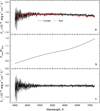 |
Fig. 1 Long-slit spectrum of comet C/2014 N3 obtained on 5 December 2015. Panel a: energy distribution in the observed spectrum of the comet (black line) and the scaled solar spectrum taken from Neckel & Labs (1984, red line). Panel b: polynomial fit of the ratio of the cometary spectrum to the solar spectrum. Panel c: emission spectrum of the comet derived by subtracting the fitted continuum from the observed spectrum. |
Observations of comet C/2014 N3 were made with the 6 m telescope BTA SAO on December 2015.
3 Analysis of observed data
3.1 Spectrum of the comet
One of the objectives of the distant comet observation program is to analyze the energy distribution in cometary spectra and identify potential molecular emissions. We combined the available spectra to enhance the signal-to-noise ratio and summed the counts within a spatial range of approximately ±9″ from the optocenter. Figure 1 illustrates the sequential transformation of the observed spectrum of comet C/2014 N3, from the raw spectrum (panel a) to the continuum and reddening (panels a, b) and, finally, to the emission spectrum (panel c). The black line in Fig. 1a represents the derived energy distribution across the observed spectrum of the comet. Given the high resolution of the solar spectrum (Neckel & Labs 1984), it was convolved using an appropriate instrumental profile to match the resolution of the cometary spectrum, and then normalized to the comet’s flux of about λ5000 Å. The procedure for calculating the continuum calculation is described in detail in our previous papers by Ivanova et al. (2018, 2019); Ivanova et al. (2021b). The resulting solar spectrum (red line) is superimposed on the observed spectrum of the comet. To isolate the emission spectrum of the comet (Fig. 1), we subtracted from the observed spectrum the fitted continuum, obtained as the reddening (Fig. 1b) multiplied by the solar spectrum.
The spectrum of comet C/2014 N3 does not exhibit typical gas emissions, including CO+ and N2+ emissions. Previously, CO+ and ![Mathematical equation: $\[\mathrm{N}_{2}^{+}\]$](/articles/aa/full_html/2025/05/aa53286-24/aa53286-24-eq1.png) ions were detected in comet C/2002 VQ94 (LINEAR) at a distance of 8.36 au from the Sun (Korsun et al. 2014) and CO+ (Ivanova et al. 2021b) at a heliocentric distance of 5.06 au.
ions were detected in comet C/2002 VQ94 (LINEAR) at a distance of 8.36 au from the Sun (Korsun et al. 2014) and CO+ (Ivanova et al. 2021b) at a heliocentric distance of 5.06 au.
Since no emissions were detected, we set upper limits for C2, C3, and NH2 fluxes and their production rates. Unfortunately, we could not determine an upper limit on the CN production rate because this spectral range is very noisy. To determine these upper limits, we used the Haser model (Haser 1957) and the same method applied to the emission-less spectrum of distant comets (Rousselot et al. 2014; Ivanova et al. 2023). We calculated the amplitudes of the minimum measurable signal, equal to the root-mean-square noise level, in the wavelength domains corresponding to the passband of narrowband comet filters (Farnham et al. 2000). Since we conducted spectral observations, the rectangular slit area was converted into a circular aperture, and the observed flux was adjusted accordingly. For calculations, we used the values for fluorescence efficiency (g-factor), parent and daughter scale lengths (lp and ld), and the power-law index n, which depends on the heliocentric distance (r−n), taken from Table 10 of Langland-Shula & Smith (2011). These upper limits are listed in Table 2.
By analyzing the spectral reflectivity of the dust, defined as the ratio of the cometary spectrum to the scaled solar spectrum, we determined the normalized spectral gradient S′(λ) for the (g–r). Usually, the normalized reflectivity gradient of cometary dust S′(λ) is used to quantify reddening in a specific wavelength range. To determine S′(λ), we used the following expression from A’Hearn et al. (1984):
![Mathematical equation: $\[S^{\prime}\left(\lambda_1, \lambda_2\right)=\frac{20}{\left(\lambda_2-\lambda_1\right)} \frac{\left(S_2-S_1\right)}{\left(S_2+S_1\right)},\]$](/articles/aa/full_html/2025/05/aa53286-24/aa53286-24-eq2.png) (1)
(1)
where S1 and S2 are reflectivities at wavelengths λ1 and λ2, respectively. Thus, we obtained a value of the normalized spectral gradient of (8 ± 1)% per 1000 Å, which agrees very well with the average value for the sample of 31 active comets found by Solontoi et al. (2012) and close to that for active long-period comets (see Fig. 10 in Jewitt 2015).
Upper limits for the main emissions in the spectrum of comet C/2014 N3.
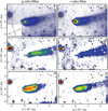 |
Fig. 2 Intensity maps of comet C/2014 N3 in the g-sdss and r-sdss filters. Panels a and b: direct images of the comet. Panels c and d: images processed by the rotational gradient method (Larson & Sekanina 1984). Panels e and f: images to which a division by the 1/ρ profile has been applied (Samarasinha & Larson 2014). The color scale does not reflect the absolute brightness of the comet. Arrows in panels e and f indicate the contaminating field stars. The arrows point toward the Sun, the north, the east, and the negative velocity vector of the comet as seen on the plane of the sky. |
3.2 Photometry of the comet
Morphology of the coma. We created intensity maps (Fig. 2) by summing all photometric images taken with the same g-sdss filter (left panel) and separately with the r-sdss filter (right panel). The cometary coma appears compact and slightly asymmetrical. The comet’s tail is wide and elongated perpendicular to the direction of the Sun. In shape, it is similar to that observed in the distant comet C/2007 D1 (LINEAR) (Ivanova et al. 2015) and in comet C/2003 WT42 (LINEAR) (Korsun et al. 2010).
To reveal low-contrast features in the dust coma of comet C/2014 N3, we applied digital filtering techniques to the images (see Figs. 2c,d). We used a combination of three numerical methods and visual inspection: the rotational gradient method (Larson & Sekanina 1984), the 1/ρ profile, and the renormalization methods (Samarasinha & Larson 2014). Each enhancement method changes the image differently, so we compared the enhanced images to exclude false features. Each technique was applied to all individual frames and the stacked image to determine the authenticity of the revealed features. We also investigated changes in structure caused by shifts in the comet’s optocenter. This approach is effective in identifying structures in different comets (Ivanova et al. 2017; Ivanova et al. 2021a, 2023; Picazzio et al. 2019; Rosenbush et al. 2017). We did not reveal any noticeable jet-like structures in the processed images.
Parameter A f ρ and color in the visible range. The parameter A f ρ is commonly used as an indicator of the rate of dust production in comets. According to A’Hearn et al. (1984), A f ρ is the product of three characteristics: the albedo (A) of dust particles; the filling factor (f), which is the ratio of the total geometric cross section of cometary dust particles to the projected cross section of a circular aperture measured at the location of the comet; and the radius (ρ) of the circular aperture. Since A and f are dimensionless parameters, the parameter A f ρ is measured in the same units as the radius ρ, usually measured in centimeters. In practice, the parameter A f ρ can be determined from the apparent magnitude of the comet, as follows from the works of A’Hearn et al. (1984) and Mazzotta Epifani et al. (2010):
![Mathematical equation: $\[A f \rho=\frac{4 r_h^2 \Delta^2}{\rho} \times 10^{0.4\left(m_{S u n}-m_c\right)}.\]$](/articles/aa/full_html/2025/05/aa53286-24/aa53286-24-eq3.png) (2)
(2)
To calculate the parameter A f ρ from (Eq. (2)), we used the apparent magnitudes and colors of the Sun from Willmer (2018). The resulting dust production rate in g-sdss and r-sdss filters is shown in Fig. 3. Calculations were performed for apertures with different radii, from 1000 to 26 000 km, but the analysis was conducted only for radii starting from 4000 km (excluding the seeing area). The spatial profiles of A f ρ through the coma in the g-sdss and r-sdss filters are uniform and similar for the two filters. The uniformity of the profiles is confirmed by the results of morphological analysis of the dust coma, which shows the absence of clearly defined active structures. As can be seen in the figure, the A f ρ values in the r-sdss band significantly exceed those measured in the g-sdss band. The same behavior of A f ρ with distance from the nucleus in different filters indicates that the properties of particles change with wavelength. According to spectral data (see Fig. 1b), the reflectivity of cometary dust rises significantly toward the red range, leading to an increase in the geometric albedo and, hence, A f ρ in the r-sdss band. A similar difference was observed in the distant comet C/2014 A4 (SONEAR) (Ivanova et al. 2019), where the wavelength-dependent variation in A f ρ and the corresponding reddening trends were also attributed to changes in dust properties.
When the cometary coma is in a steady state, the value of A f ρ should be constant over the coma and independent of the aperture. However, in comet C/2014 N3, the parameter A f ρ is not constant with cometocentric distance. The A f ρ value varies from 830 ± 70 (out of the range of seeing) at ρ ≈ 5000 km to the maximum value approximately 900 ± 80 cm at ρ ≈ 11 000 km for the r-sdss filter and, from 715 ± 65 to 780 ± 70 cm for the g-sdss filter. Such variations in A f ρ across the coma are usually attributed to non-steady-state dust emission and/or if optical properties of dust grains vary within the coma due to sublimation or fragmentation. Possible dust grain fading cannot also be excluded.
Both profiles show a sharp increase in A f ρ up to approximately 11 000 km from the cometary optocenter, part of which is possibly affected by the seeing, which is limited by the dashed line in Fig. 3, and then is a quite slow decrease with increasing cometocentric distance ρ. More or less similar trends in A f ρ across the coma are observed in both short-period comets (e.g., Mazzotta Epifani & Palumbo 2011) and long-period comets (Mazzotta Epifani et al. 2014; Sun et al. 2024). However, the best similarity in the A f ρ profiles (in value and trend) is observed for comets C/2014 N3 and C/2008 FK75 (Lemmon-Siding Spring), which was observed at a heliocentric distance of 5.01 au by Mazzotta Epifani et al. (2014). Indeed, the r-sdss A f ρ value, derived for comet C/2014 N3 in the reference aperture of ρ = 104 km and centered on the optocenter, is 910 ± 60 cm, and R-band A f ρ for comet C/2008 FK75 in the corresponding aperture is 895 ± 72 cm (Mazzotta Epifani et al. 2014). According to these A f ρ values, both comets are moderately active. Indeed, as shown in Fig. 4, the average A f ρ parameters in the optical and near-IR ranges in an aperture with a radius of 10 000 km, obtained in this work for comet C/2014 N3 in the range of heliocentric distances of 4–5 au, are close to the lower limit of values for long-period comets at similar distances.
To create a color map of comet C/2014 N3, we converted each pixel of the stacked g-sdss and r-sdss images to an apparent magnitude. After this, we created a final color map (g–r) by subtracting the two sets of images from each other (Fig. 5). The average measurement error of magnitude is 0.03m. Analyzing the color map obtained, one can see that the dust color (g–r) in comet C/2014 N3 is predominantly red. The low signal-to-noise ratios in the tail and field stars prevent us from concluding with certainty that there is a significant color change there. Using magnitudes obtained in apertures and rings of different sizes, we estimated the dust color in comet C/2014 N3 (Fig. 6). As can be seen from the figure, the dust color measured by both methods practically does not change in the inner coma (0.69m ± 0.06m), indicating a rather homogeneous coma in color up to ~6000 km from the optocenter. However, the observed change in the g-r color with increasing distance from the nucleus falls within the uncertainties suggesting that it may not be a significant effect. This homogeneity is apparently due to the absence of strong active structures in the coma, which have been observed in other distant comets. In general, the distribution of dust color in comet C/2014 N3 differs from what we observed (Ivanova et al. 2019; Ivanova et al. 2021b, 2023).
Compared to the literature data, several characteristic features observed in comets can be highlighted. According to studies by Solontoi et al. (2012) for various types of comets and Holt et al. (2024) for long-period comets, despite the diversity of their physical and dynamical properties, the photometric colors of comets are relatively uniform (g − r = 0.57m ± 0.05m from Solontoi et al. 2012 and g − r = 0.51m ± 0.03m from Holt et al. 2024) and do not correlate with their main characteristics. Solontoi et al. (2012) suggested that this uniformity might indicate that light scattering in the coma is primarily influenced by large dust particles, similar to those found in cometary nuclei and Jupiter Trojans. Regarding our results, the color of comet C/2014 N3 is 0.69m ± 0.06m, which is somewhat higher than the values mentioned above. However, for unresolved comets such as 19P/Borrelly and 174P/Echeclus (Solontoi et al. 2012), the g – r color reaches ~0.7m, which can be attributed to the limited resolution of photometric observations, where the measured color reflects either the nucleus or an unresolved coma. In particular, this conclusion is supported by Ivanova et al. (2021b) for comet C/2011 KP36 (Spacewatch) and aligns with the suggestion by Jewitt (2015) that cometary evolution results in the gradual loss of ultra-red material from the nucleus surface due to activity, exposing more neutral or blue material. Thus, the red color of a comet may indicate its recent transition from the outer Solar System, where activity has not yet altered its spectral properties. Kwon et al. (2024) studied comet C/2017 K2 (Pan-STARRS) and detected transient color changes at ~2.9 au, characterized by sequential bluing and reddening of both the inner and outer coma, followed by a return to the initial values by ~2.5 au. These variations may result from temporary changes in the composition or properties of dust near the water-ice sublimation boundary. Additionally, comet C/2022 E3 (ZTF) also exhibited (Adami et al. 2023) an anomalously red coma color g − r = 0.75m, which could be caused either by gas contamination in the r-band (e.g., NH2) or by the presence of relatively large dust particles (Kolokolova et al. 2001). Thus, the observed color characteristics of the cometary coma reflect a complex interplay of dust, gas, and evolutionary processes, emphasizing the need for further studies in this field.
Parameter A f ρ and CO and CO2 production rate in IR. As described in detail by Bauer et al. (2015), each NEOWISE visit-stack of the W1 (3.4 μm) and W2 (4.6 μm) images was analyzed for IR excess (Fig. 7). The W1 images were used to constrain the reflected light contribution from the dust, while the thermal contribution of the dust was modeled as an aggregate of large (>3 μm) dust grains with equivalent surface area. We note that the thermal signal contribution of the nucleus in the two NEOWISE bands in Fig. 7 at the distances where comet C/2014 N3 was observed was negligible. Results, including 3.4 μm A f ρ in cm units and proxy CO2 production rates (Q(CO2); cf. Bauer et al. 2015; Gicquel et al. 2023) in units of molecules per second, are shown in Table 3. The A f ρ value in the table is given for the 11 arcsec aperture (about 31 000 km), while for the 6 arcsec aperture A f ρ = (370 ± 85) cm, and 9 arcsec apertures (392 ± 94) cm. As one can see, the values overlap. A comparison of A f ρ values in the visible range and at a wavelength of 3.4 μm shows that the 3.4 μm observations, which were taken a few months earlier, yielded lower values. The Q(CO2) rates assume that the IR excess in W2 is completely attributable to the production of CO2 species alone. However, the NEOWISE photometry cannot differentiate between the CO (4.67 μm) and CO2 (4.23 μm) emission bands within the 4.6 μm channel, so comet C/2014 N3 could alternatively emit CO or both species. The production rate of CO, if that is the dominant species, would be ~11 times greater than the CO2 shown in Table 3.
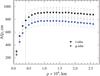 |
Fig. 3 Dependence of the parameter A f ρ on the aperture radius projected onto comet C/2014 N3 in the g-sdss and r-sdss filters. The near-nucleus area, which may be affected by seeing, is delimited by the vertical dotted line and was not considered. |
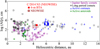 |
Fig. 4 Comparison of average A f ρ parameter in comet C/2014 N3 and other active small bodies (A’Hearn et al. 1995; Hui et al. 2017; Jewitt 2005; Korsun et al. 2014, 2016; Lamy et al. 2009; Lowry et al. 1999; Lowry & Fitzsimmons 2001; Lowry & Weissman 2003; Lowry & Fitzsimmons 2005; Mazzotta Epifani et al. 2007, 2009a,b, 2014, 2016; Schleicher et al. 1997; Shubina et al. 2023; Snodgrass et al. 2006; Szabó et al. 2001; Rousselot et al. 2016, 2021; Voitko et al. 2022; Wong et al. 2019). |
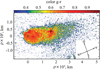 |
Fig. 5 Color map (g–r) of comet C/2014 N3 obtained from images taken on 5 December 2015 using the g-sdss and r-sdss filters. The arrow indicates contaminating field stars. The rest of the designations are the same as in Fig. 2. |
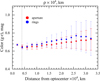 |
Fig. 6 Variations in the color of dust in the coma of comet C/2014 N3 measured through different apertures and rings about 0.7″ wide. The near-nucleus area, which may be affected by seeing, is delimited here by the vertical dashed line and was not considered. |
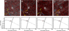 |
Fig. 7 Stacked images of comet C/2014 N3 for the four NEOWISE visits with significant signals (see Table 3); on 4 July 2014 (Panel a), 13 December 2014 (Panel b), 8 August 2015 (Panel c), and 10 January 2016 (Panel d). For each panel, the 3.4 μm band stacked image is mapped to the blue and green channels, and the 4.6 μm stacked image is mapped to the red. The N and E sky directions are labeled, along with the antisolar vector (in red) and the anti-velocity vector (in blue). The photometry from NEOWISE observations of comet C/2014 N3 for each visit is shown below the stacked image. The fluxes from emissions at 3.4 μm (red triangle) and 4.6 μ (black diamond) are shown. The reflected light model (dotted line), thermal model (solid line), and combined signal (dashed line) are overplotted. |
Dust and W2 excess measurements for comet C/2014 N3 as observed by NEOWISE.
4 Monte Carlo dust tail modeling
To retrieve the dust’s physical properties and loss rate, we used our forward Monte Carlo dust tail code (see Moreno 2022, and references therein). The BTA image taken through the r-sdss filter is the most appropriate for this analysis since it is the least possibly contaminated by molecular emissions. The code is only applicable to the region at a distance outward of about 20Rn (Rn is a nucleus radius), where the nucleus gravity and the gas drag force can be neglected. Thus, the initial particle speeds refer actually to the terminal speeds at such distances. The particle orbits are Keplerian, since they are affected by the solar gravity and radiation pressure forces only. The code computes the trajectories of such particles, which depend on their initial velocity and the so-called β parameter; it can be expressed as ![Mathematical equation: $\[\beta=\frac{C_{\mathrm{pr}} Q_{\mathrm{pr}}}{2 \rho_{\mathrm{d}} r}\]$](/articles/aa/full_html/2025/05/aa53286-24/aa53286-24-eq4.png) , where Cpr = 1.19 × 10³ kg m−2 is the radiation pressure coefficient, Qpr is the scattering efficiency for radiation pressure, taken as unity (Burns et al. 1979), ρd is the particle density, assumed to be 1000 kg m−3, and r is the particle radius. The heliocentric position of each particle is computed at the observation date, and projected onto the sky plane. In the Monte Carlo procedure, a large number (≳ 107) of particles are simulated, whose brightness is a function of their size and geometric albedo, assumed at pv = 0.04, a customary value for comet dust. The phase function effect is made through a linear phase coefficient of 0.03 mag deg−1. Both the geometric albedo and the phase coefficient values are in the range of those measured by Meech & Jewitt (1986, 1987). The final synthetic brightness image, being a function of the assumed mass-loss rate and size distribution, is computed as the sum of the contribution of all the sampled particles. This distribution is taken as a power-law function limited by minimum and maximum radii (rmin and rmax) and a certain power exponent, κ (i.e.,
, where Cpr = 1.19 × 10³ kg m−2 is the radiation pressure coefficient, Qpr is the scattering efficiency for radiation pressure, taken as unity (Burns et al. 1979), ρd is the particle density, assumed to be 1000 kg m−3, and r is the particle radius. The heliocentric position of each particle is computed at the observation date, and projected onto the sky plane. In the Monte Carlo procedure, a large number (≳ 107) of particles are simulated, whose brightness is a function of their size and geometric albedo, assumed at pv = 0.04, a customary value for comet dust. The phase function effect is made through a linear phase coefficient of 0.03 mag deg−1. Both the geometric albedo and the phase coefficient values are in the range of those measured by Meech & Jewitt (1986, 1987). The final synthetic brightness image, being a function of the assumed mass-loss rate and size distribution, is computed as the sum of the contribution of all the sampled particles. This distribution is taken as a power-law function limited by minimum and maximum radii (rmin and rmax) and a certain power exponent, κ (i.e., ![Mathematical equation: $\[n(r) \propto \int_{r_{\text {min }}}^{r_{\text {max }}} r^{\kappa}\]$](/articles/aa/full_html/2025/05/aa53286-24/aa53286-24-eq5.png) ). In addition to the dust brightness, we also considered the brightness contribution from the comet nucleus, which is assumed to be located at the image photocenter, and has the same geometric albedo and linear phase coefficient as those of the particles. The only free parameter is a nucleus radius, Rn, to be determined during the tail fitting procedure.
). In addition to the dust brightness, we also considered the brightness contribution from the comet nucleus, which is assumed to be located at the image photocenter, and has the same geometric albedo and linear phase coefficient as those of the particles. The only free parameter is a nucleus radius, Rn, to be determined during the tail fitting procedure.
To find the best possible fit to the observed tail, the method is necessarily a trial-and-error procedure. Since there is only one available image, and given the large number of free parameters of the model, the solution cannot unfortunately be unique. We rely on previous typical determinations of physical parameters found for other comets to obtain a set of parameters that could give a reasonable fit to the observed image. Thus, in addition of the parameters already described, we fixed the power-law index to κ = −3.5, and the limiting radii of the size distribution to rmin = 1 μm and rmax = 1 cm. These values are in the range of those retrieved by dust tail analysis for several comets (see Fulle 2004). We then searched for the best-fitting velocity and mass-loss-rate functions. The velocity is parameterized by a function of β and the heliocentric distance as ![Mathematical equation: $\[v=v_{0} \sqrt{\beta / r_{\mathrm{h}}}\]$](/articles/aa/full_html/2025/05/aa53286-24/aa53286-24-eq6.png) , where v0 is expressed in km s−1 and rh is expressed in au (Whipple 1951). The dust mass-loss rate was set to a Gaussian function with peak production rate occurring sometime relative to perihelion, t0, and a certain FWHM.
, where v0 is expressed in km s−1 and rh is expressed in au (Whipple 1951). The dust mass-loss rate was set to a Gaussian function with peak production rate occurring sometime relative to perihelion, t0, and a certain FWHM.
In addition to the BTA image, another source of information on the activity of this comet comes from magnitude measurements, available from the Minor Planet Center (MPC), as well as from amateur observations, specifically from Cometas_Obs2, a group of enthusiastic amateur astronomers that have provided photometric and image data of many comets since the 1990s. These photometric measurements would help us better constrain the model parameters, owing to their large temporal coverage, −250 to +650 days since perihelion, as will be described below.
Before starting the analysis with the Monte Carlo model, we built a synchrone map (Finson & Probstein 1968), which provided us with a zeroth-order constraint on emission times from the comet. Figure 8 gives different synchrones overplotted on the image brightness contours. The synchrone ages are −1000, −600, −400, −200, 0 (the perihelion synchrone, shown as a dashed line), +100, +200, and +250, in clockwise order. From this diagram, we can say that the comet was significantly active since ~1000 days pre-perihelion, lasting at least till the BTA image observation time ~268 days post-perihelion.
We start the modeling procedure by considering the most simple scenario, which corresponds to an isotropic ejection model with the above mentioned parameters. After repeated experimentation with the model we arrived at the fit shown in Fig. 9. In this plot and subsequent image, the synthetic image has been convolved with a Gaussian function to mimic the seeing effect. The best fit image, is shown compared with the observation by a contour map (panel a) and a brightness profile along the tail, in the direction of the blue dashed line (panel b). This fit corresponds to the dust loss rate as a function of time displayed in panel c, which peaks 300 days before perihelion (t0 = −300 days), with maximum at 700 kg s−1, and with a FWHM of the Gaussian of FWHM = 700 days. The velocity parameter v0 was found at v0 = 125 m s−1. We found that a nucleus radius of Rn = 15 ± 3 km fits very well the brightness levels near the photocenter, although we emphasize that it is only a weakly constrained parameter. This radius will remain fixed for all the models described below. As shown in Fig. 9, while the overall fit to the image is good, the model isophotes do not capture very well the observed shapes. Then, to check whether an improvement is possible, a second attempt to model the image was made by changing the emission pattern to a more realistic scenario where the ejection is limited to the illuminated portion of the spherical nucleus and with the ejection velocity proportional to the cosine of the solar zenith angle, z, with no emission from the nightside. In Fig. 10, we see that this sunward ejection model constitutes a better fit to the observed isophotes. The only difference between the isotropic and sunward models is the addition of the term cos z to the expression of the velocity; v0 is now v0 = 0.25 km s−1, twice the value of the isotropic ejection model, to account for the term cos z. The equation of the velocity for this sunward model is therefore ![Mathematical equation: $\[v=v_{0} \sqrt{\beta / r_{\mathrm{h}}} ~\cos~ z\]$](/articles/aa/full_html/2025/05/aa53286-24/aa53286-24-eq7.png) , with v0 = 0.25 km s−1. The same dependence of speed on particle size, heliocentric distance, and solar zenith angle was proposed by Kelley et al. (2009) in their dynamical modeling of the dust ejected from comet 67P/Churyumov-Gerasimenko at 5.5–4.3 au from the Sun, although with v0 = 0.5 km s−1 (i.e., a factor of two higher than what we find for C/2014 N3).
, with v0 = 0.25 km s−1. The same dependence of speed on particle size, heliocentric distance, and solar zenith angle was proposed by Kelley et al. (2009) in their dynamical modeling of the dust ejected from comet 67P/Churyumov-Gerasimenko at 5.5–4.3 au from the Sun, although with v0 = 0.5 km s−1 (i.e., a factor of two higher than what we find for C/2014 N3).
In our model, a r = 1 μm particle would have v ~100 m s−1 at noon at perihelion, while for a 1 cm particle the velocity would be 1 m s−1. These speeds are in line to those found by Mazzotta Epifani et al. (2016) for comet C/2009 P1 (Garradd) at large heliocentric distances. Table 4 summarizes all the best-fit model parameters, specifying whether they were assumed or derived in the analysis.
To constrain the model parameters more accurately, we used the photometric data, which span a long time baseline, and ran the tail model for such dates to obtain synthetic r-sdss band magnitudes. The magnitude determinations come from two sources, the MPC, and the amateur group Cometas_Obs. From the MPC we take only the measurements labeled as “nucleus magnitudes” since they refer to the circumnuclear region only. In Fig. 11, panel c, those measurements are plotted as tiny black dots. The scatter is large, so to minimize this scatter we performed an average of every 4 days, shown as green dots. On the other hand, the measurements performed by Cometas_Obs are obtained through R-band filters and are represented by brown dots. These measurements are directly comparable with our modeled r-sdss magnitudes, which are close to the R-band photometric data (the expected magnitude differences between the two filters are minimal, less than 0.2 mag, which is completely negligible in this context). The average of MPC magnitudes and those by Cometas_Obs are quite consistent, and provide a reliable brightness evolution for comparison. In this sense, we run the Monte Carlo model for all the observation dates by Cometas_Obs, and calculated the synthetic magnitudes at each date, using the same apertures as provided by the amateur observers. Then, for the sunward ejection model, we obtained the curves shown in thick red lines in panel c. We see that the magnitudes are reasonably well reproduced from −50 to +650 days to perihelion, except for the time span between −50 and +100 days, where no data were taken, and we cannot confirm the agreement. However, the model predicts an excess of brightness when we project it to earlier dates, between 250 and 50 days pre-perihelion. Although the excess is not very large (always less than a magnitude), we tried to improve the fit by varying one-by-one each of the model parameters. The only possibility that we found of doing this without affecting severely the quality of the fit to the observed image contours was by varying the dust mass-loss rate as indicated in the blue line of the panel c in Fig. 10. We tried to improve the fits by adjusting each of the model parameters one by one, in particular the dust loss rate as a function of time, which we found to be the most influential parameter on the final result. This was accomplished by testing tens of functions, by modifying the initial gaussian profile with piecewise functions producing similar total dust mass ejection. With this mass-loss-rate profile, the fit to the magnitude light curve clearly improves (as indicated by the blue line of panel c in Fig. 11); the fit to the tail, although worse than that with the Gaussian profile, it is still acceptable (blue contours in panel b of Fig. 11). A possible reason for this loss rate dependence being more abrupt with respect to the Gaussian profile is a seasonal effect, but we do not have other observations that could provide further insight into this phenomenon. In fact, the same seasonal argument could be invoked to explain the fact of having the maximum production rate before perihelion. However, the total dust production is very similar for the two dust loss rate profiles, 4.5 × 10¹⁰ kg and 4.9 × 10¹⁰ kg, respectively. The peak dust mass-loss rate of about 700 kg s−1 is similar to that of 29P/Schwassmann-Wachmann 1 at about 6 au (Fulle 1992; Moreno 2009). A similar production rate of ~500 kg s−1 was derived by Fulle et al. (1998) for comet C/1995 O1 Hale-Bopp but at a much larger heliocentric distance of 13 au. The diversity in production rates for long-period comets is clearly shown by Mazzotta Epifani et al. (2014) who, out of a sample of seven long-period comets at large heliocentric distances (5–8.5 au), they obtained production rates ranging from 30 to 1400 kg s−1.
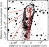 |
Fig. 8 Isophote and synchrone map corresponding to BTA image of comet C/2014 N3 in the r-sdss filter. Isophotes are shown as black contours, and from the outermost to the innermost they are 24.5, 24, 23, 22, and 21 mag arcsec−2. Synchrones (in red) point approximately from south to east and (going clockwise) correspond to −1000, −600, −400, −200, 0 (perihelion synchrone, dashed line), +100, +200, and +250 days relative to perihelion. All images shown in this section are in the standard orientation: north is up, east to the left. |
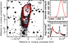 |
Fig. 9 Isophote fields, dust loss rate profiles, and brightness scans along the tail of the C/2014 N3 BTA image in the r-sdss filter. In panel a, the black contours are the observed isophotes, with the same brightness levels as in Fig. 8. The red contours are the isophotes corresponding to the isotropic ejection model, whose dust loss rate profile is given in panel c. In panel a, the dashed blue line indicates the direction of the brightness scans along the tail, shown in panel b as a black line (observation) and a red line (isotropic ejection model). The spikes indicated by arrows are contaminating field stars. |
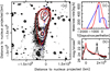 |
Fig. 10 Isophote fields, dust loss rate profiles, and brightness scans along the tail of the C/2014 N3 BTA image in the r-sdss filter. In panel a, the black contours are the observed isophotes, with the same brightness levels as in Fig. 8. The red contours are the isophotes corresponding to the sunward ejection model, whose dust loss rate profile is given as the red line in panel c. The solid blue line in panel c corresponds to the modified dust loss rate to account for the magnitude measurements in Fig. 11. In panel a, the dashed blue line indicates the direction of the brightness scans along the tail, shown in panel b as the black line (observation) and the red line (sunward ejection model). |
Physical parameters of the best-fit dust ejection model.
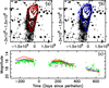 |
Fig. 11 Comparisons of the observed and model isophotes and of the synthetic magnitudes, both as a function of time to perihelion. In panel a, black contours are the observed isophotes, and red contours the sunward ejection model, with the dust loss rate profile shown in red in panel c of Fig. 10. In panel b, the black contours are the observed isophotes, and the blue contours correspond to the same sunward model as in panel a, but with the modified dust loss rate profile shown as the blue line in panel c of Fig. 10. Isophote levels in panels a and b are the same as in Fig. 8, and the axis labels are also expressed in km. Panel c displays the C/2014 N3 magnitude as a function of time extracted from the Minor Planet Center (“nuclear magnitudes”; little black dots). Also, the moving averages of these measurements are shown using 4-day-width boxes (green dots) and the R-band measurements by Cometas_Obs (brown dots). The red lines correspond to the magnitudes modeled using the sunward ejection model with the Gaussian profile (red line in Fig. 10), while the blue line corresponds to the sunward profile with the modified dust loss rate profile (blue line in Fig. 10). |
5 Conclusions
In this paper we have presented the results of a comprehensive analysis of observations of the distant comet C/2014 N3. These observations were made with the 6 m BTA telescope on 5 December 2015 at a heliocentric distance of 4.51 au, approximately 268 days after perihelion. In the coma, which was asymmetrical and slightly elongated in the direction of the comet’s motion, we do not find any pronounced jet-like structures, only a long dust tail. The A f ρ parameter, a proxy of the dust production rate in the comet, obtained in the r-sdss band, varied through the coma and tail from 830 to 900 cm within distances from 5000 to 11000 km and then remained almost constant, ~900 cm, up to distances of 26 000 km. The comet’s color map (g–r) shows a homogeneously red dust coma with no significant color variations along the tail. On average, the dust color index (g–r) is about 0.7m.
In addition, we analyzed NEOWISE observations of comet C/2014 N3 taken at rh = 4.45 and 3.96 au (inbound) and at rh = 4.09 and 4.68 au (outbound) in the two IR bands, 3.4 μm (W1) and 4.6 μm (W2). It appears that the A f ρ parameter obtained from the W1 stacked images slightly increases as the comet approaches perihelion and then gradually decreases as the comet moves away; however, we cannot assert this with confidence because the errors in A f ρ are quite large. On average, A f ρ is about 370 cm in the 3.4 μm band. The difference between the visible A f ρ value and the IR value is most likely due to either the lower reflectivity of the particles at a wavelength of 3.4 μm or the presence of a significant fraction of submicron particles.
We do not detect typical gas emissions of C2, C3, or NH2, nor CO+ or N2+, in the cometary spectrum. We have established upper limits for the fluxes and production rates of C2, C3, and NH2 molecules but could not determine the production rate of CN due to noise in this spectral range. The calculated upper limits for these molecules are relatively low. Via our analysis of dust reflectivity, we find a reddening gradient of approximately 8% per 1000 Å. According to NEOWISE data, the production rate of CO2 molecules correlates with the heliocentric distance; in other words, as the comet approaches perihelion, the Q(CO2) value increases to (3.0 ± 0.4) × 1026 mol s−1 at r = 3.96 au and after perihelion decreases to (1.6 ± 0.4) × 1026 mol s−1 at r = 4.68 au. Due to the low spectral resolution in the 4.6 μm band, it is impossible to separate the contributions of CO and CO2, so we can only assume that if the signal in that band comes from CO rather than CO2, the Q(CO) value would be 11 times greater than that for CO2 molecules. Overall, comet C/2014 N3 has lower dust and gas production rates than other long-period comets (Pinto et al. 2022; Reach et al. 2013). Its CO2 production rate is notably lower than that of comets like C/1995 O1 (Hale-Bopp) and C/2016 R2 (Pan-STARRS). However, comets 269P/Jedicke, 273P Pons–Gambart, P/2012 B1 (Pan-STARRS), C/2013 G6 (Lemmon), and 2014 Q1 (Pan-STARRS) Gicquel et al. (2023) have production rates similar to those of C/2014 N3 at similar distances. In contrast, comets such as 103P and 19P (Reach et al. 2013) and centaur 39P (Pinto et al. 2023) exhibit production rates lower than those of C/2014 N3. These differences suggest that C/2014 N3 may have a distinct composition (for example, less volatile content), nucleus size, or number of active areas compared to more CO2-rich comets. CO and CO2 are the primary carbon-bearing molecules in cometary comae and play a key role in driving their activity. Their relative abundances impose important constraints on models of Solar System formation and evolution. According to Pinto et al. (2022), CO2 dominates over CO in most studied comets, particularly among Jupiter-family comets, whereas in the outer regions of the Solar System (beyond 3.5 au), CO-dominated comae are more common. This may be related to prolonged cosmic irradiation of the nucleus surface. Recent JWST observations of 39P/Oterma (Pinto et al. 2023) also confirm the presence of CO2.
The Monte Carlo dust tail modeling of comet C/2014 N3 allowed us to estimate key physical parameters. The model reproduces the observed comet magnitudes well between 250 days before perihelion and 650 days after perihelion. However, an excess brightness was observed on earlier dates, which was corrected for by modifying the dust mass-loss rate. So, the peak dust production occurred around 300 days before perihelion, with a maximum mass-loss rate of approximately 700 kg s−1, which is within the range of dust production rates of other observed long-period comets at large heliocentric distances. The total dust mass loss is estimated to be around 4.5–4.9 × 10¹⁰ kg. The isotropic dust ejection model produces an acceptable fit to the observations, but the sunward directed ejection model provides a better fit to the observed isophotes. The latter assumes that ejection occurs from the illuminated side of the nucleus, which improved the fit considerably. For particles with a radius of 1 μm, the velocity was about 100 m s−1 at perihelion, while for 1 cm particles, it was about 1 m s−1. Our study shows that dust ejection occurred over an extended period, starting 1000 days before perihelion and continuing until 268 days after perihelion.
Acknowledgements
We thank the amateur association Cometas_Obs for providing us with photometric data for C/2014 N3 (NEOWISE). F.M. acknowledges financial supports from grants PID2021-123370OB-I00, and from the Severo Ochoa grant CEX2021-001131-S funded by MICIU/AEI/10.13039/501100011033. This research has made use of data provided by the International Astronomical Union’s Minor Planet Center. The Monte Carlo dust tail code makes use of the JPL Horizons ephemeris generator system. The work by OI was supported by the Slovak Grant Agency for Science VEGA (Grant No. 2/0059/22) and by the Slovak Research and Development Agency under Contract No. APVV-19-0072. The research of V.R. and I.L. was supported by the projects of the Ministry of Education and Science of Ukraine No. 25BF023-01 and No. 0124U001304. We thank the anonymous reviewer and the editor for their helpful and constructive feedback.
References
- Adami, C., Jehin, E., Aravind, K., et al. 2023, in Les Journées de la SF2A [Google Scholar]
- Afanasiev, V., & Amirkhanyan, V. 2012, Astroph. Bull., 67, 438 [Google Scholar]
- A’Hearn, M. F., Schleicher, D. G., Millis, R. L., Feldman, P. D., & Thompson, D. T. 1984, AJ, 89, 579 [Google Scholar]
- A’Hearn, M. F., Millis, R. C., Schleicher, D. G., Osip, D. J., & Birch, P. V. 1995, Icarus, 118, 223 [CrossRef] [Google Scholar]
- Bauer, J. M., Stevenson, R., Kramer, E., et al. 2015, AJ, 814, 85 [Google Scholar]
- Burns, J. A., Lamy, P. L., & Soter, S. 1979, Icarus, 40, 1 [Google Scholar]
- Cutri, R. M., Mainzer, A., Conrow, T., et al. 2015, Explanatory Supplement to the NEOWISE Data Release Products, Explanatory Supplement to the NEOWISE Data Release Products, http://wise2.ipac.caltech.edu/docs/release/neowise/expsup [Google Scholar]
- Farnham, T. L., Schleicher, D. G., & A’Hearn, M. F. 2000, Icarus, 147, 180 [Google Scholar]
- Finson, M. L., & Probstein, R. F. 1968, ApJ, 154, 327 [NASA ADS] [CrossRef] [Google Scholar]
- Fulle, M. 1992, Nature, 359, 42 [Google Scholar]
- Fulle, M. 2004, Comets II (Tucson: University of Arizona Press), 1, 565 [Google Scholar]
- Fulle, M., Cremonese, G., & Böhm, C. 1998, AJ, 116, 1470 [Google Scholar]
- Gicquel, A., Bauer, J. M., Kramer, E. A., Mainzer, A. K., & Masiero, J. R. 2023, Planet. Sci. J., 4, 3 [Google Scholar]
- Haser, L. 1957, Bulletin de la Societe Royale des Sciences de Liege, 43, 740 [NASA ADS] [Google Scholar]
- Henden, A. A., Templeton, M., Terrell, D., et al. 2016, VizieR Online Data Catalog: II [Google Scholar]
- Holt, C. E., Knight, M. M., Kelley, M. S., et al. 2024, Planet. Sci. J., 5, 273 [Google Scholar]
- Hui, M.-T., Jewitt, D., & Clark, D. 2017, AJ, 155, 25 [CrossRef] [Google Scholar]
- Ivanova, O., Neslušan, L., Krišandová, Z. S., et al. 2015, Icarus, 258, 28 [Google Scholar]
- Ivanova, O., Rosenbush, V., Afanasiev, V., & Kiselev, N. 2017, Icarus, 284, 167 [Google Scholar]
- Ivanova, O. V., Picazzio, E., Luk’yanyk, I. V., Cavichia, O., & Andrievsky, S. M. 2018, Planet. Space Sci., 157, 34 [Google Scholar]
- Ivanova, O., Luk’yanyk, I., Kolokolova, L., et al. 2019, A&A, 626, A26 [NASA ADS] [CrossRef] [EDP Sciences] [Google Scholar]
- Ivanova, O., Luk’yanyk, I., Tomko, D., & Moiseev, A. 2021a, MNRAS, 507, 5376 [Google Scholar]
- Ivanova, O., Rosenbush, V., Luk’yanyk, I., et al. 2021b, A&A, 651, A29 [NASA ADS] [CrossRef] [EDP Sciences] [Google Scholar]
- Ivanova, O., Rosenbush, V., Luk’yanyk, I., et al. 2023, A&A, 672, A76 [NASA ADS] [CrossRef] [EDP Sciences] [Google Scholar]
- Jewitt, D. 2005, AJ, 129, 530 [NASA ADS] [CrossRef] [Google Scholar]
- Jewitt, D. 2015, AJ, 150, 201 [NASA ADS] [CrossRef] [Google Scholar]
- Kartasheva, T., & Chunakova, N. 1978, Astrofiz. Issled. Izv. Spets. Astrofiz. Obs, 10, 44 [Google Scholar]
- Kelley, M. S., Wooden, D. H., Tubiana, C., et al. 2009, AJ, 137, 4633 [NASA ADS] [CrossRef] [Google Scholar]
- Kolokolova, L., Jockers, K., Gustafson, B. Å., & Lichtenberg, G. 2001, J. Geophys. Res. Planets, 106, 10113 [Google Scholar]
- Korsun, P. P., Kulyk, I. V., Ivanova, O. V., et al. 2010, Icarus, 210, 916 [NASA ADS] [CrossRef] [Google Scholar]
- Korsun, P. P., Rousselot, P., Kulyk, I. V., Afanasiev, V. L., & Ivanova, O. V. 2014, Icarus, 232, 88 [NASA ADS] [CrossRef] [Google Scholar]
- Korsun, P. P., Ivanova, O. V., Afanasiev, V. L., & Kulyk, I. V. 2016, Icarus, 266, 88 [NASA ADS] [CrossRef] [Google Scholar]
- Kulyk, I., Rousselot, P., Korsun, P., et al. 2018, A&A, 611, A32 [NASA ADS] [CrossRef] [EDP Sciences] [Google Scholar]
- Kwon, Y. G., Bagnulo, S., Markkanen, J., et al. 2024, AJ, 168, 164 [Google Scholar]
- Lamy, P., Toth, I., Weaver, H., A’Hearn, M., & Jorda, L. 2009, A&A, 508, 1045 [NASA ADS] [CrossRef] [EDP Sciences] [Google Scholar]
- Langland-Shula, L. E. & Smith, G. H. 2011, Icarus, 213, 280 [CrossRef] [Google Scholar]
- Larson, S., & Sekanina, Z. 1984, AJ, 89, 571 [NASA ADS] [CrossRef] [Google Scholar]
- Lowry, S., & Fitzsimmons, A. 2001, A&A, 365, 204 [NASA ADS] [CrossRef] [EDP Sciences] [Google Scholar]
- Lowry, S., & Fitzsimmons, A. 2005, MNRAS, 358, 641 [Google Scholar]
- Lowry, S. C., & Weissman, P. R. 2003, Icarus, 164, 492 [NASA ADS] [CrossRef] [Google Scholar]
- Lowry, S., Fitzsimmons, A., Cartwright, I., & Williams, I. 1999, A&A, 349, 649 [Google Scholar]
- Masci, F. 2013, Astrophysics Source Code Library [record ascl:1302.010] [Google Scholar]
- Mazzotta Epifani, E., & Palumbo, P. 2011, A&A, 525, A62 [NASA ADS] [CrossRef] [EDP Sciences] [Google Scholar]
- Mazzotta Epifani, E., Palumbo, P., Capria, M., et al. 2007, MNRAS, 381, 713 [Google Scholar]
- Mazzotta Epifani, E., Palumbo, P., Capria, M., et al. 2009a, A&A, 502, 355 [NASA ADS] [CrossRef] [EDP Sciences] [Google Scholar]
- Mazzotta Epifani, E., Palumbo, P., & Colangeli, L. 2009b, A&A, 508, 1031 [NASA ADS] [CrossRef] [EDP Sciences] [Google Scholar]
- Mazzotta Epifani, E., Dall’Ora, M., Di Fabrizio, L., et al. 2010, A&A, 513, A33 [NASA ADS] [CrossRef] [EDP Sciences] [Google Scholar]
- Mazzotta Epifani, E., Perna, D., Di Fabrizio, L., et al. 2014, A&A, 561, A6 [NASA ADS] [CrossRef] [EDP Sciences] [Google Scholar]
- Mazzotta Epifani, E., Snodgrass, C., Perna, D., et al. 2016, Planet. Space Sci., 132, 23 [NASA ADS] [CrossRef] [Google Scholar]
- Meech, K. J., & Jewitt, D. C. 1986, ESA SP, 250, 553 [Google Scholar]
- Meech, K. J., & Jewitt, D. C. 1987, A&A, 187, 585 [NASA ADS] [Google Scholar]
- Meech, K. J., Pittichová, J., Bar-Nun, A., et al. 2009, Icarus, 201, 719 [NASA ADS] [CrossRef] [Google Scholar]
- Moreno, F. 2009, ApJS, 183, 33 [Google Scholar]
- Moreno, F. 2022, Universe, 8, 366 [NASA ADS] [CrossRef] [Google Scholar]
- Neckel, H., & Labs, D. 1984, Sol. Phys., 90, 205 [Google Scholar]
- Oke, J. 1990, AJ, 99, 1621 [NASA ADS] [CrossRef] [Google Scholar]
- Picazzio, E., Luk’yanyk, I. V., Ivanova, O. V., et al. 2019, Icarus, 319, 58 [NASA ADS] [CrossRef] [Google Scholar]
- Pinto, O. H., Womack, M., Fernandez, Y., & Bauer, J. 2022, Planet. Sci. J., 3, 247 [NASA ADS] [CrossRef] [Google Scholar]
- Pinto, O. H., Kelley, M., Villanueva, G., et al. 2023, Planet. Sci. J., 4, 208 [Google Scholar]
- Reach, W. T., Kelley, M. S., & Vaubaillon, J. 2013, Icarus, 226, 777 [CrossRef] [Google Scholar]
- Rosenbush, V. K., Ivanova, O. V., Kiselev, N. N., Kolokolova, L. O., & Afanasiev, V. L. 2017, MNRAS, 469, S475 [NASA ADS] [CrossRef] [Google Scholar]
- Rousselot, P., Korsun, P., Kulyk, I., et al. 2014, A&A, 571, A73 [NASA ADS] [CrossRef] [EDP Sciences] [Google Scholar]
- Rousselot, P., Korsun, P., Kulyk, I., Guilbert-Lepoutre, A., & Petit, J.-M. 2016, MNRAS, 462, S432 [NASA ADS] [CrossRef] [Google Scholar]
- Rousselot, P., Kryszczyńska, A., Bartczak, P., et al. 2021, MNRAS, 507, 3444 [NASA ADS] [CrossRef] [Google Scholar]
- Samarasinha, N. H., & Larson, S. M. 2014, Icarus, 239, 168 [NASA ADS] [CrossRef] [Google Scholar]
- Schleicher, D. G., Lederer, S. M., Millis, R. L., & Farnham, T. L. 1997, Science, 275, 1913 [Google Scholar]
- Shubina, O., Kleshchonok, V., Ivanova, O., Luk’yanyk, I., & Baransky, A. 2023, Icarus, 391, 115340 [Google Scholar]
- Shubina, O., Ivanova, O., Petrov, D., et al. 2024, MNRAS, 528, 7027 [NASA ADS] [CrossRef] [Google Scholar]
- Snodgrass, C., Lowry, S. C., & Fitzsimmons, A. 2006, MNRAS, 373, 1590 [NASA ADS] [CrossRef] [Google Scholar]
- Solontoi, M., Ivezić, Z., Jurić, M., et al. 2012, Icarus, 218, 571 [CrossRef] [Google Scholar]
- Sun, S., Shi, J., Ma, Y., & Zhao, H. 2024, MNRAS, 529, 1617 [Google Scholar]
- Szabó, G. M., Csák, B., Sárneczky, K., & Kiss, L. L. 2001, A&A, 374, 712 [NASA ADS] [CrossRef] [EDP Sciences] [Google Scholar]
- Voitko, A., Zubko, E., Ivanova, O., et al. 2022, Icarus, 388, 115236 [NASA ADS] [CrossRef] [Google Scholar]
- Whipple, F. L. 1951, ApJ, 113, 464 [NASA ADS] [CrossRef] [Google Scholar]
- Willmer, C. N. A. 2018, ApJS, 236, 47 [Google Scholar]
- Wong, I., Mishra, A., & Brown, M. E. 2019, AJ, 157, 225 [Google Scholar]
All Tables
Observations of comet C/2014 N3 were made with the 6 m telescope BTA SAO on December 2015.
All Figures
|
Fig. 1 Long-slit spectrum of comet C/2014 N3 obtained on 5 December 2015. Panel a: energy distribution in the observed spectrum of the comet (black line) and the scaled solar spectrum taken from Neckel & Labs (1984, red line). Panel b: polynomial fit of the ratio of the cometary spectrum to the solar spectrum. Panel c: emission spectrum of the comet derived by subtracting the fitted continuum from the observed spectrum. |
| In the text | |
|
Fig. 2 Intensity maps of comet C/2014 N3 in the g-sdss and r-sdss filters. Panels a and b: direct images of the comet. Panels c and d: images processed by the rotational gradient method (Larson & Sekanina 1984). Panels e and f: images to which a division by the 1/ρ profile has been applied (Samarasinha & Larson 2014). The color scale does not reflect the absolute brightness of the comet. Arrows in panels e and f indicate the contaminating field stars. The arrows point toward the Sun, the north, the east, and the negative velocity vector of the comet as seen on the plane of the sky. |
| In the text | |
|
Fig. 3 Dependence of the parameter A f ρ on the aperture radius projected onto comet C/2014 N3 in the g-sdss and r-sdss filters. The near-nucleus area, which may be affected by seeing, is delimited by the vertical dotted line and was not considered. |
| In the text | |
|
Fig. 4 Comparison of average A f ρ parameter in comet C/2014 N3 and other active small bodies (A’Hearn et al. 1995; Hui et al. 2017; Jewitt 2005; Korsun et al. 2014, 2016; Lamy et al. 2009; Lowry et al. 1999; Lowry & Fitzsimmons 2001; Lowry & Weissman 2003; Lowry & Fitzsimmons 2005; Mazzotta Epifani et al. 2007, 2009a,b, 2014, 2016; Schleicher et al. 1997; Shubina et al. 2023; Snodgrass et al. 2006; Szabó et al. 2001; Rousselot et al. 2016, 2021; Voitko et al. 2022; Wong et al. 2019). |
| In the text | |
|
Fig. 5 Color map (g–r) of comet C/2014 N3 obtained from images taken on 5 December 2015 using the g-sdss and r-sdss filters. The arrow indicates contaminating field stars. The rest of the designations are the same as in Fig. 2. |
| In the text | |
|
Fig. 6 Variations in the color of dust in the coma of comet C/2014 N3 measured through different apertures and rings about 0.7″ wide. The near-nucleus area, which may be affected by seeing, is delimited here by the vertical dashed line and was not considered. |
| In the text | |
|
Fig. 7 Stacked images of comet C/2014 N3 for the four NEOWISE visits with significant signals (see Table 3); on 4 July 2014 (Panel a), 13 December 2014 (Panel b), 8 August 2015 (Panel c), and 10 January 2016 (Panel d). For each panel, the 3.4 μm band stacked image is mapped to the blue and green channels, and the 4.6 μm stacked image is mapped to the red. The N and E sky directions are labeled, along with the antisolar vector (in red) and the anti-velocity vector (in blue). The photometry from NEOWISE observations of comet C/2014 N3 for each visit is shown below the stacked image. The fluxes from emissions at 3.4 μm (red triangle) and 4.6 μ (black diamond) are shown. The reflected light model (dotted line), thermal model (solid line), and combined signal (dashed line) are overplotted. |
| In the text | |
|
Fig. 8 Isophote and synchrone map corresponding to BTA image of comet C/2014 N3 in the r-sdss filter. Isophotes are shown as black contours, and from the outermost to the innermost they are 24.5, 24, 23, 22, and 21 mag arcsec−2. Synchrones (in red) point approximately from south to east and (going clockwise) correspond to −1000, −600, −400, −200, 0 (perihelion synchrone, dashed line), +100, +200, and +250 days relative to perihelion. All images shown in this section are in the standard orientation: north is up, east to the left. |
| In the text | |
|
Fig. 9 Isophote fields, dust loss rate profiles, and brightness scans along the tail of the C/2014 N3 BTA image in the r-sdss filter. In panel a, the black contours are the observed isophotes, with the same brightness levels as in Fig. 8. The red contours are the isophotes corresponding to the isotropic ejection model, whose dust loss rate profile is given in panel c. In panel a, the dashed blue line indicates the direction of the brightness scans along the tail, shown in panel b as a black line (observation) and a red line (isotropic ejection model). The spikes indicated by arrows are contaminating field stars. |
| In the text | |
|
Fig. 10 Isophote fields, dust loss rate profiles, and brightness scans along the tail of the C/2014 N3 BTA image in the r-sdss filter. In panel a, the black contours are the observed isophotes, with the same brightness levels as in Fig. 8. The red contours are the isophotes corresponding to the sunward ejection model, whose dust loss rate profile is given as the red line in panel c. The solid blue line in panel c corresponds to the modified dust loss rate to account for the magnitude measurements in Fig. 11. In panel a, the dashed blue line indicates the direction of the brightness scans along the tail, shown in panel b as the black line (observation) and the red line (sunward ejection model). |
| In the text | |
|
Fig. 11 Comparisons of the observed and model isophotes and of the synthetic magnitudes, both as a function of time to perihelion. In panel a, black contours are the observed isophotes, and red contours the sunward ejection model, with the dust loss rate profile shown in red in panel c of Fig. 10. In panel b, the black contours are the observed isophotes, and the blue contours correspond to the same sunward model as in panel a, but with the modified dust loss rate profile shown as the blue line in panel c of Fig. 10. Isophote levels in panels a and b are the same as in Fig. 8, and the axis labels are also expressed in km. Panel c displays the C/2014 N3 magnitude as a function of time extracted from the Minor Planet Center (“nuclear magnitudes”; little black dots). Also, the moving averages of these measurements are shown using 4-day-width boxes (green dots) and the R-band measurements by Cometas_Obs (brown dots). The red lines correspond to the magnitudes modeled using the sunward ejection model with the Gaussian profile (red line in Fig. 10), while the blue line corresponds to the sunward profile with the modified dust loss rate profile (blue line in Fig. 10). |
| In the text | |
Current usage metrics show cumulative count of Article Views (full-text article views including HTML views, PDF and ePub downloads, according to the available data) and Abstracts Views on Vision4Press platform.
Data correspond to usage on the plateform after 2015. The current usage metrics is available 48-96 hours after online publication and is updated daily on week days.
Initial download of the metrics may take a while.