| Issue |
A&A
Volume 665, September 2022
|
|
|---|---|---|
| Article Number | A79 | |
| Number of page(s) | 11 | |
| Section | Planets and planetary systems | |
| DOI | https://doi.org/10.1051/0004-6361/202142902 | |
| Published online | 14 September 2022 | |
Physical properties and mini-outburst of 64P/Swift-Gehrels
1
Purple Mountain Observatory, Chinese Academy of Sciences,
Nanjing
210023, PR China
e-mail: This email address is being protected from spambots. You need JavaScript enabled to view it.
2
School of Astronomy and Space Science, University of Science and Technology of China / Institute of Deep Space Sciences, Deep Space Exploration Laboratory,
Hefei
230026, PR China
3
Key Laboratory of Planetary Sciences, Chinese Academy of Sciences,
Nanjing
210023, PR China
4
CAS Center for Excellence in Comparative Planetology,
Hefei
230026, PR China
Received:
14
December
2021
Accepted:
4
July
2022
Abstract
Aims. We present secular multiwavelength broadband photometry, spanning over 93 days, performed at the Yaoan High Precision Telescope on comet 64P/Swift-Gehrels in its 2018–2019 apparition. Our aim is to study its dust activity, coma properties, and the accidentally discovered mini-outburst.
Methods. We used aperture photometry to measure the Afρ value and correct the back-scattering effect based on phase angle. We deployed azimuthally averaged image enhancement methods to identify the coma morphology and the outburst. Secular color measurement was also conducted on the comet.
Results. We identified a −0.5 mag mini-outburst around January 3, 2019, with coma morphology study showing an obvious dust jet feature strengthened during the outburst. The maximum A(0)fρ value of 64P/Swift-Gehrels recorded is 313 cm at the top of the fitted curve and 334 cm at the outburst event. Both volatile-driven pressure mechanisms and nonvolatile-driven mechanisms could be the major explanation for the outburst. We obtain a mean color B − V = 0.68 ± 0.03 and V − R = 0.08 ± 0.01. The B − V color is similar to the mean value for Jupiter Family comets, but the V − R color turns out to be bluest among all the recorded short-period comets. The cause of this anomaly remains unknown.
Key words: comets: general / comets: individual: 64P/Swift-Gehrels / methods: observational / techniques: photometric
© R. Q. Xu et al. 2022
 Open Access article, published by EDP Sciences, under the terms of the Creative Commons Attribution License (https://creativecommons.org/licenses/by/4.0), which permits unrestricted use, distribution, and reproduction in any medium, provided the original work is properly cited.
This article is published in open access under the Subscribe-to-Open model. This email address is being protected from spambots. You need JavaScript enabled to view it. to support open access publication.
1 Introduction
Comets are considered to be a group of small bodies originating in the proto-solar disk that formed our Solar System. For most of their lives they wander in the farthest regions, but sometimes trespassers may come to the inner Solar System due to dynamical evolutions. Unlike asteroids, they preserve a large amount of volatiles that sublimate from their surface while exposed to the solar radiation, which forms their active nature. The gas and dust continually released from the surface of the cometary nucleus produce a gravitationally unbound atmosphere, called the coma. For an active comet, most of its brightness is contributed by the coma.
Comets have been observed systematically over the past few decades, and have been classified into different subsets. One key parameter to define these population subsets is the orbital period. An arbitrary classification defines short-period comets as comets with orbital periods of less than 20 yr, while intermediate comets have orbital periods of 20–200 yr, and long-period comets over 200 yr (Tancredi et al. 2006). This classification is still in use for the Minor Planet Center (MPC). There is another classification that uses the Tisserand constant of Jupiter Tj. This convenient parameter defines a special subset within the observed comet population, the Jupiter Family Comets (JFC). The Jupiter-family comets are a type of comets whose dynamical evolution is controlled by Jupiter. To distinguish JFCs from other types of comets, JFCs have Tj > 2 while Halley-type comets (roughly equal to the intermediate-period comets mentioned above) and long-period comets have Tj > 2 (Vaghi 1973). Most of the discovered JFCs fit the definition of short-period comets (Fernández et al. 1999).
Comet 64P/Swift-Gehrels (hereafter 64P) was poorly investigated in the past. Its discovery dates to November 17, 1889, when L. Swift found an object of cometary appearance at Warner Observatory. It was not observed again until Tom Gehrels used the 122 cm Schmidt telescope at Palomar Mountain Observatory to claim its rediscovery on February 8, 1973. In its most recent 2018–2019 apparition, 64P reached its perihelion distance of 1.39 au on November 3, 2018. Its orbital period is 9.41 yr and its Tj = 2.495, so 64P should be characterized as a JFC. Two catalogs investigating the nuclear magnitude of comets include 64P. In the catalog presented by Tancredi et al. (2006), the nucleus size of 64P is 1.8 km, while in the catalog from the Jet Propulsion Laboratory (JPL) Small-Body Database, the nucleus size of 64P is 1.6 km. In its 2018–2019 apparition, 64P was in a favorable position for observation as it made a close approach to the Earth and its geometry condition allowed months of continual observations near perihelion. Several outbursts of this comet were observed in this apparition (Kelley et al. 2019), and our own observations indicate another outburst around January 3, 2019.
The phenomenon of cometary outburst is quite common among comets. 29P/Schwassmann-Wachmann is a typical comet for having numerous recorded outburst events (Roemer 1958; Jewitt 1990; Trigo-Rodríguez et al. 2008). The outburst means the brightness of the comet suddenly rises from lower than 1 mag to higher than 5 mag for largest outbursts. Afterward, the brightness possibly falls back to the level before the outburst. During the outburst the cometary nucleus emits a large amount of cometary material into space, giving rise to the magnitude variation. With these material increments, the inner coma expands to replace the old diffuse coma before the outburst, thus the coma may change its shape in a few days, resulting in a possibly asymmetrical coma. The volatile-driven mechanisms for outbursts are discussed by Gronkowski & Wesołowski (2016); the mini-outburst without significant gas emission increment that the Rosetta mission observed in situ on 67P/Churyumov-Gerasimenko (hereafter 67P) gave rise to nonvolatile-driven mechanisms such as landslides and avalanches (Kelley et al. 2021). So far, none of the mechanisms can fully explain the morphology presented in the outburst, but it is commonly agreed that the direct reasons for cometary outbursts is the massive explosive ejection of surface material of the nucleus (Gronkowski & Wesołowski 2016).
Section 2 contains the data reduction of the broadband observations. In Sect. 3, we present observational results and discuss the physical properties of comet 64P. Further discussions on color and outburst are found in Sect. 4. The conclusions are summarized in Sect. 5.
Observation log.
2 Observation and data reduction
The JFC 64P was observed with the Yaoan High Precision Telescope (YAHPT) (IAU code O49). The telescope is located at the Purple Mountain Observatory Yaoan Station in Yunnan Province, southwest China. It is an 80 cm Ritchey-Chretien telescope, equipped with a 2048 x 2048 pixel2 PI CCD camera. The field of view (FOV) of this telescope is 11.8 arcmin2. The spatial resolution for each axis is 0.347″ per pixel. We used the Johnson–Kron–Cousins B, V, R broadband filters for our observation. The long-term observation lasted 44 nights in total from October 25, 2018, around the perihelion of 64P to February 12, 2019, when it was 1.82 au away from the Sun. All the astrometric data are queried from Minor Planet Center (MPC), and the observational geometry of the circumstances are summarized in Table 1.
Limited by the apparent velocity of the comet, the exposure time of the observation was restricted to avoid the condition that the cometary proper motion was greater than the standard seeing of the observation site of 1.3″ in each image. After bias subtraction, flat-fielding, and removal of cosmic rays, we used aperture photometry on the images to derive the magnitude of the comet. The aperture was set to 6000 km on the cometary nucleus instead of the traditional 10000 km (the standard scale for a JFC coma) because on this apparition 64P was so close to Earth (with the minimum distance of 0.445 au) that the aperture size of 10 000 km covered a large area of sky, which may cause frequent nearby star contamination. In addition, we used a fixed 6000 km aperture size throughout the observations to provide comparable photometric results, because although the Afp value remains unchanged in theory, it varies with different aperture used (Tozzi et al. 2003). Sky correction was performed with a first-order polynomial sky approximation using pixel areas far enough away from the stars or possible coma contamination on the same image. The data reduction was done by IRAF, and flux calibration was done with the help of the Aladin Skymap and UCAC4 Catalog. For detailed investigations of coma morphology, we applied a two-dimensional Gaussian fitting to find the optocenter of the comet, realigned those images using the optocenter, and co-added the image with the same filter in one night to enhance the signal-to-noise ratio.
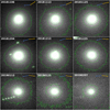 |
Fig. 1 Co-added R-band images of 64P on various imaging dates (as labeled). The Y-axes are realigned to the northern direction, and east is to the left. The field of view is approximately 1′ × 1′ for each image. The yellow arrow represents the Sun’s direction, while the blue arrow represents the velocity direction of the comet. |
3 Result
3.1 Visual appearance
The close geocentric distance of 64P in its 2018–2019 apparition allowed its coma to cover a radius of 0.5′ across the sky. A series of selected co-added images of 64P are shown in Fig. 1. These images are taken from YAHPT with R-band filter. The visual appearances of the coma are all nearly circular in our observational data, with a little stretch close to the opposite direction to the comet-to-Sun vector, which is supposed to be the direction of the dust tail. We adopt the dust tail model to explain the round shape visual appearance in Sect. 4.1.
3.2 Afp
The activity of a comet is a distinct feature among all the celestial bodies. The major contributors of the visual brightness of comets from optical broadband observations are the dust particles, which are produced along with the volatile sublimation. The precise way to measure the activity of a comet is to determine its mass loss rate, including volatile sublimation and dust ejection. However, the precise value of dust production rate is highly model-dependent (Shi et al. 2019), so we adopt the Afρ value that A’Hearn et al. (1984) presented as a proxy for cometary activity measurement, where A is the grain albedo, f is the filling factor in the field of view, and ρ is the aperture in the photometric reduction. This proxy can be derived as
 (1)
(1)
where rh is the heliocentric distance, Δ is the geocentric distance, ms is the solar magnitude, and mc is the comet magnitude calculated within the aperture of radius ρ in R band.
The Afρ value varies when the comet moves inbound or outbound, showing the change in dust activity level of the coma. Generally, the activity reaches its peak value around perihelion where the comet receives the most heat from the Sun. The peak may delay for a month or more for some comets because their presumed older devolatilized surface shows a thermal lag effect to reach maximum activity (Meech & Svoren 2004). A few comets can show a peak in activity before perihelion because of the seasonal effect, for example 21P/Giacobini-Zinner in the past apparition (Ehlert et al. 2019). Mass loss events such as outburst and splitting of the comets could result in an abrupt change in cometary activity, creating another peak in the Afρ curve. Since the R band covers the spectral range where the volatile emissions are weak for the comets, the Afρ value using photometric observations through the R-band filter can represent the dust activity. In an ideal coma with steady-state emission, the Afρ value is independent of the aperture for the photometric reduction, but a monotonic decrease is commonly reported with the aperture increase, reflecting nonsteady-state emission or possible dust grains fading or destruction (Lara et al. 2004; Tozzi et al. 2003).
The scattering efficiencies of dust particles in the comae that vary with phase angle contribute to the change in brightness and the Afρ value of the comets. An early construction of scattering phase function model was made by Divine (1981) in application to the observations of 1P/Halley. However, this phase function was proven to be not very accurate when the phase angle is too small (α < 15°) or too large (α > 90°; Schleicher et al. 1998). Further studies of the scattering phase function provide more precise matches to comet observations. Schleicher & Bair (2011) made a composite model combining his model for small phase angles with the Marcus model developed for large phase angles (Marcus 2007), which has been widely adopted in the photometric studies of comets. Bertini et al. (2017) used the OSIRIS camera on the Rosetta mission to measure the scattering phase function of 67P; this result correlates with research on other comets. Generally, the function exhibits a U-shaped structure, with a small peak at back-scattering angle (phase angle α close to 0°) and a much stronger increase at forward-scattering directions (phase angle α > 120°). For most comets observed on Earth, including 64P, the phase angle is restricted to a small range, except for the sun-grazed comets or close-approach events. In our observations, the phase angle of 64P monotonically increases from 22° to 31°, the scattering efficiencies of dust particles monotonically decrease while the phase angle increases, and the variation in our adjustment using different available models is negligible. To compare the Afρ values obtained at different phase angles, it is essential to normalize the Afρ value to a certain phase angle to provide more convincing results of dust activity (Kolokolova et al. 2001). We adopted the Schleicher-Marcus model (Schleicher & Bair 2011; Marcus 2007)1 to adjust the Afρ value to 0° phase angle, called the A(0)fρ. Because the phase angles of our observations are not close to zero, the optical brightness increase from the back-scattering effect is not obvious.
The coma magnitudes derived by aperture photometry for all the filters are listed in Table 2. The computed A(0)fρ values are plotted in Fig. 2. The red polynomial fit curve suggests that the A(0)fρ curve generally increased to a maximum point around 40 days after perihelion. However, we cannot determine the exact date when the comet was the most active, due to the lack of observational data. In addition, our only observation near the natural activity peak on December 13, 2018, seemed to be an outlier with the polynomial fit. The A(0)fρ value reached a peak of around 320 cm. We also note that on January 3 and 4, 2019, the measured A(0)fρ value was apparently higher than the fitting curve, around 20 days after the maximum point. We estimate that this could be a cometary outburst that happened around January 3, 2019.
Multiwavelength broadband photometry result for 6000 km aperture.
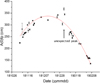 |
Fig. 2 A(0)fρ curve throughout the whole observations. The arrow indicates the data points apart from the fitting curve, which is an unexpected peak of estimated outburst. |
3.3 Morphology
Though it is acknowledged that the coma is mostly isotropic, many different asymmetric features were found covered by the isotropic emission of the coma (Rahe et al. 1969). We extracted these revealed coma features by applying some techniques, and thus we were able to start the coma morphology study. These features represent the anisotropic nature of the coma, reflecting spatial and time variations as the result of some physical processes related to coma, nucleus, and solar radiation (Boehnhardt & Birkle 1994). Through morphology studies we can reveal some physical properties of the unresolved nucleus, investigate the interaction of dust and gas in the coma, and measure the activity of the nucleus. Farnham (2009) described different types of coma features, including the commonly seen fans and jets, and the arcs, halos, shells, envelopes, and spirals that require some special geometry conditions or azimuthal perspectives to form. As for JFCs, on average they experienced longer evolution than other types of comets (Johnson et al. 1987), thus it reduces the mean activity level for this kind of comets, and the coma features of JFCs likely show less complexity compared to the highly active long-period comets. However, the extent of devolatilization of each JFC is still highly different, depending on its perihelion distance, aphelion distance, and dynamical age.
Since the special features in the coma can represent the dust activity of the comet, it is also possible that these features are sensitive to the abrupt change in the comet dust activity. As a diverged peak structure was identified in the A(0)fρ curvature apart from the regular maximum, which may stand for the outburst, morphology studies are necessary to analyze the coma features related to the peak structure. Thus, methods of image enhancement are required to study the detailed morphology in the coma covered by the mostly isotropic background of the coma dust particles. Operative methods to reveal coma features have been well categorized and used in the past (Samarasinha & Larson 2014; Birkle & Boehnhardt 1992). We thus selected the azimuthally averaged method that removes an azimuthally averaged background to show the anisotropic dust features for the coma.
To test if there was an outburst event that happened around January 3, we show the R-band observation images for January 1, 3, 4, and 11, 2019, in Fig. 3. We can clearly see the significant change in the coma morphology even for the plain image within just ten days. For a detailed investigation we used azimuthally averaged methods for image enhancement. Only simple patterns are shown in the morphology study; the major patterns shown are a diffuse fan in the anti-solar direction and a small jet in the solar direction. As Fig. 4 shows, for January 1 and January 11 the fan soon became diffuse as the distance to the nucleus increased. However, on January 3 the fan dramatically strengthened and did not show any sign of dispersion until the edge of the image 30″ away from the nucleus, the aperture for the morphology study. Instead, on January 4 this fan was still evident, but clearly weaker than the previous day. On January 11 this fan once again showed a weak pattern near the nucleus and quickly dispersed, suggesting that the effect of the outburst on the cometary activity had vanished. The coma morphology variation in these days shows the basic prospect for comet outburst. It should be noted that the enhancement techniques we used create significant errors when the distance to the nucleus is large, so the detail of the coma feature away from the nucleus could be meaningless. However, this method is still valid in judging if there was an outburst going on in the case of 64P.
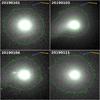 |
Fig. 3 Co-added R-band images of 64P on January 1 (upper left), January 3 (upper right), January 4 (bottom left), and January 11 (bottom right), 2019. The Y-axes are realigned to the northern direction, and east is to the left. The field of view is approximately 1′ × 1′ for each image. The yellow arrow represents the Sun’s direction, while the blue arrow represents the velocity direction of the comet. |
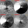 |
Fig. 4 R-band images of 64P after applying azimuthally averaged methods on January 1 (upper left), January 3 (upper right), January 4 (bottom left), and January 11 (bottom right), 2019. The Y-axes are realigned to the northern direction and east is to the left. The field of view is approximately 1′× 1′ for each image. The yellow arrow represents the Sun’s direction, while the blue arrow represents the velocity direction of the comet. |
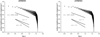 |
Fig. 5 Surface brightness profiles of 64P on January 1 (left, before outburst) and January 3 (right, after outburst), 2019, in R filter. The diagonal lines in the lower left of each panel indicate gradients m = −1 and m = −3/2 for visual reference. The linear fit is made with data between 3000 km aperture and 10 000 km aperture |
3.4 Surface brightness profile
Though a morphology study can reflect the pattern change in an outburst, image enhancement method cannot quantify the instability in the coma and its effect. The surface brightness profile can reveal the status of the coma (Jewitt & Meech 1987). For a simple steady-state coma, according to the fountain model hypothesis (Finson & Probstein 1968), the surface brightness profile follows the relationship of ρ−1 (Gehrz & Ney 1992). However, even if the coma is in a steady-state, other physical processes such as the radiation pressure or possible disintegration of the dust particles can reduce the index of the relationship below −1. For most comets recorded, the index of the surface brightness profiles lies in the range from −1 to −2; however, if the index is below −1.5, the only explanation can be the occurrence of nonsteady-state emission (Lowry et al. 1999).
During our observations we obtained R-band images with signal-to-noise ratio values high enough to compute the one-dimensional surface brightness profile. Because the water ice sublimation on the comet tends to be steady if the activity presented by the A(0)fρ value remains unchanged, the surface brightness profile also tends to stay the same. A simple comparison of the surface brightness profile on different dates can reveal the comparative stability of the coma emission, which is presented in Fig. 5. For January 1, 2019, a linear least-squares fit to the surface brightness profile from 1.3″ (i.e., outside the area affected by the seeing) to 10″ gives a slope of m = −0.92 ± 0.05. This slope is consistent with a steady-state coma for comet 64P. For January 3, 2019, when an outburst was believed to have happened, the fitting gives a slope of m = −0.91 ± 0.05. This slope is almost the same as the slope measured before outburst, and is also consistent with steady-state emission in the coma of 64P. This plot shows that this outburst is a very weak one that has a negligible effect on the stability of the coma, and thus the coma remains stable within the outburst. An extended examination of the surface brightness profiles on the other days with observational data yielded similar fitting slopes, suggesting the stability of the 64P coma did not have long-term variation during our observations.
3.5 Color
Our multiwavelength broadband observation was carried out with Johnson-Kron-Cousins broadband B, V, R filters. The data we obtained through these broadband filters mainly reflect the strength of the continuum part in the spectrum rather than the emission lines of the gas species. The sunlight reflected by the dust particles in the coma is the major contributor of the continuum part of the cometary spectrum (Blackwell & Willstrop 1957). The strength of the dust component varies with the activity of the comet, but the response for the activity in different bands could be different, and thus the color of the comet may show short-term or long-term variation (Betzler et al. 2017). As the cometary color is also relevant to the material composition of the comet, a unique color is suggested for comets in different dynamical categories (Jewitt 2015). For comparative study among JFCs, we may use color to reveal the unique features of 64P.
The data obtained during the observations allowed us to analyze the coma color of the target comets. Table 2 summarizes the color obtained at the optical aperture of radius ρ = 6000 km, chosen to minimize the effects of the sky background and possible contamination of nearby star light. The mean color of 64P we measured is B − V = 0.68 ± 0.03, V − R = 0.08 ± 0.01. While the mean color of active JFCs is B − V = 0.75 ± 0.02, V − R = 0.47 ± 0.02, the mean color of JFCs nuclei is B − V = 0.87 ± 0.05, V − R = 0.50 ± 0.03, and the solar color is B − V = 0.64 ± 0.02, V − R = 0.35 ± 0.01 (Jewitt 2015; Lamy & Toth 2009; Solontoi et al. 2012; Holmberg et al. 2006). The B − V value for 64P is similar to the mean value of the JFCs, but the V − R value for 64P is far less than the mean value, which means the 64P seems bluer than most of the JFCs and the Sun. This phenomenon is rare because most comets tend to be redder than the Sun in the past observations, possibly due to the effect of space weathering (Bertini 2011; Solontoi et al. 2012; Betzler et al. 2017; Lowry et al. 1999, 2003).
4 Discussion
4.1 Model
The dynamical behavior of dust particles in the coma is different depending on the region they reside in. In the innermost coma the motion of dust particles is so complex that it requires advanced hydrodynamic models to solve the coupling between sublimating gas and ejected dust, and it is sensitive to the boundary conditions of the nucleus. However, in the outer part of the coma the motion of dust particles is assumed to be insensitive to boundary conditions and it is mainly controlled by gravity and the radiation pressure of the Sun. The dust tail structure for this scenario was described in depth in the Finson-Probstein model (Finson & Probstein 1968).
Based on the description of Fulle et al. (2004, 2010) and the FP-like model on the Internet service Comet-toolbox2 (Finson & Probstein 1968; Vincent 2014), we used a Monte Carlo model to simulate the dust environment of 64P. The dust grains are uniquely characterized by β, the ratio of solar gravity to the solar radiation pressure for each dust particle. In our model, a large number of dust particles with different β values are released from the cometary nucleus a 0.01 day intervals. The velocities of these particles are randomly distributed to cover all the solid angles. The total number of particles ejected in the entire simulation is 3 × 10⁹, which is enough to make the number of dust particles obey the distribution and the direction of the emission could be considered isotropic. The motion of dust particles in the outer coma can be described as
 (2)
(2)
Several constraints are adopted to the input dust properties. A power-law size distribution function with power index α, a free parameter in our model, is assumed to be the size distribution function of dust particles valid for the whole 2018–2019 apparition. The lower and upper limits of the radii are set to 0.1µm and 1 cm, similar to the setup of previous models (Fulle 1989; Moreno et al. 2004) and the average radius of dust particles would be ~10 µm, consistent with the observation of comets (Jewitt 2009). The number of grains produced in each release is derived from a normalized heliocentric distance dependent dust production rate, which is converted from the Afρ value previously obtained by the photometric results (see Sect. 3.2), with a model described in Rousselot et al. (2014). The heliocentric distance dependency is roughly estimated to be  , suggesting that the activity of 64P is very sensitive to its heliocentric distance. In addition, a −2.6 magnitude outburst on August 14, 2018 (Kelley et al. 2019), is adopted as the start of cometary activity in the simulation. The dust production rate before the outburst is negligible because the secular photometric data from MPC and Seiichi Yoshida’s aerith.net web page3 suggest that the brightness of 64P did not seem to fall back to the level before the outburst. The terminal velocity of dust particles at the boundary of the dust-gas decoupling region is proportional to
  (Crifo 1991) as the dust-gas interaction model for the innermost coma indicates. We adopted the estimate of velocity in Li et al. (2013) that the terminal velocity of dust particles in our model should be
 (3)
(3)
where rh is the distance to the Sun in au, f is the other free parameter to vary our estimate of the terminal velocity, and the velocity is in meters per second.
The dust properties of 64P in our model are represented by two free parameters, the power index of size distribution function α and the scaling factor of terminal velocity f. To derive the free parameters, we fit the morphology of the observed coma to the simulated synthetic coma. Figure 6 shows the best fit isophote contour plot of the observation (left panel) and the simulation (right panel) for the observation on January 1, 2019. The best fit combination of the two free parameters is f = 2.6 and α = −3.4. It suggests that for 64P the velocity of dust particles is higher than we expected, and large particles contribute slightly more to the brightness of the coma than small particles. The synthetic picture also shows that a nearly round coma can be formed with the geometry condition of 64P at that time instead of the stereotypical coma-tail structure. However, for the case of outbursts our isotropic emission model cannot reproduce the significant bulge in the southeast (Fig. 3, upper right panel). It may indicate that the possible variation in a power-law index or terminal velocity in the outburst could not account for the observed bulge alone. We suspect that the features in the outburst could be attributed to the anisotropic emission that constantly existed in our observations, manifested by the fan and jet shown with azimuthally averaged methods (see Sect. 3.3). In the steady emission, the observed coma still could be fitted well by an isotropic model, showing that the extent of anisotropy was weak for 64P that did not experience outburst. In the situation of outburst, the coma morphology on January 3, 2019, was affected by a stronger anisotropic emission, and our isotropic model cannot reproduce similar patterns. Figure 4 also shows that the features representing anisotropic emission were clearly intensified, consistent with our conclusion that the outburst was originated by the strengthening anisotropic emission, possibly from the region that was already active on the surface.
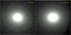 |
Fig. 6 Isophote contour plot of the R-band observed coma (left) and the simulated dust coma (right) on January 1, 2019. The field of view is approximately 1′× 1′’ for each image. The contour lines correspond to 21.5, 20.8, 20.4, and 20.0 mag arcsec-2. |
4.2 Magnitude variation and mechanisms of the outburst
Though the outburst was proven to exist and investigated with several means, the origin of the outburst still remains unsolved.
Because the brightness of the comet always rises to the maximum soon after the outburst, it is impossible to determine the precise magnitude variation without the knowledge of the exact moment of the outburst. And we spotted no clear sign of outburst in pre-outburst observations. The Afρ measurement from the Spanish association Cometas-Obs4 recorded higher activity up to 300 cm (658 cm if adjusted to zero phase angle) on January 2, 2019, indicating that the outburst may have taken place one day before our observation of the outburst on January 3. So we were not fortunate enough to observe a developing morphological outburst feature in the coma, and the strength of the dust activity had been decaying since the outburst event. The outburst morphology we observed probably shows the afterglow of the outburst, and thus we cannot obtain the exact magnitude variation in the outburst. However, a rough estimate could be given combining our observations and data from Cometas-Obs that the outburst of 64P on January 2, 2019, varied the R-band brightness by Δm = −0.5 magnitude, and that it should be categorized as a mini-outburst.
Volatile-driven mechanisms were interpreted as the cause of the phenomenon of cometary outbursts for several tens of years. In general, this kind of mechanism indicates a scenario that the volatile pressure down to several meters beneath the surface layer overwhelms the nucleus surface tensile strength. Outbursts or mini-outbursts with these origins are related to events that strengthen the volatile pressure or weaken the surface tensile. Volatile pressure could be boosted by astrochemical processes like the crystallization of the amorphous ice (Gronkowski & Wesołowski 2016), which occurs in shallow subsurfaces of 0.5 to several meters (Marboeuf & Schmitt 2014). Other mechanisms lead to the weakening surface tensile, such as the collision with meteors or solar activity. We checked the public released data from Solar Eruptive Event Detection System (SEEDS)5 and found no significant solar activity several days before the outburst; therefore, it is unlikely that normal solar wind could easily break through the nucleus surface, otherwise outbursts should be a much more frequent event for comets. The collision mechanism produces similar phenomena with the boosting of volatile pressure (Holsapple 1993), but it is restricted by the collision frequency of small bodies (Gronkowski 2004). The resulting outbursts would be either the opening of a vent exposing the internal volatile reservoir to surface or the explosion that destroys the surface layer, depending on whether the following volatile-driven activity exists or not (Knollenberg et al. 2016). In our case, the coma pattern clearly created by outburst survived for at least two days and faded gradually, indicating the existence of follow-up activity. So, the most likely volatile-driven mechanism for the outburst we observed could be that the pressurized gas breached the surface layer and created significant dust ejection on the nucleus.
Furthermore, the mini-outburst on 67P with no significant increase in CO2 and H2O sublimation observed by the Rosetta mission (Rinaldi et al. 2016) gave rise to another origin of cometary outbursts that does not require pressurized volatiles. Steckloff & Melosh (2016) suggested that this outburst could originate from avalanches. In addition, Pajola et al. (2017) found an “ambiguous link” between the cliff collapse (Vincent et al. 2016) and another outburst observed on 67P by the Rosetta mission. However, without narrowband observational data to check the change in the gas emission, we can hardly get proof for the above nonvolatile-driven mechanisms based on ground observations of comets, let alone determine if the comet has a rough surface to support this sort of mechanism. It is likely that with rough terrain, outbursts with nonvolatile-driven mechanisms would happen repeatedly on an active comet. For another outburst research on 67P, Agarwal et al. (2017) stated that the nonvolatile-driven mechanisms could be triggering volatile-driven mechanisms by undermining the strength of the nucleus surface and could allow the pressurized gas to breach. This could also be one of the possibilities for the origin of the outburst on 64P.
It is also worth mentioning that in August, 2018, three months prior to our observations, four outbursts were identified for 64P with magnitude variation ranging from −0.2 to −2.6 magnitude in the Sloan Digital Sky Survey (SDSS) r band (Kelley et al. 2019). Together with our observations, it shows that the 64P was observed experiencing five outbursts within half a year, despite the insufficient observation coverage. Compared with the six outbursts that 46P/Wirtanen (hereafter 46P) experienced in the recent favorable apparition, it is reasonable to suspect that 64P shares similar intermediate outburst frequency with 46P (Kelley et al. 2021). However, the effective radius of the nucleus of 64P was measured to be 1.6 km or 1.8 km (see Sect. 1), while 46P has a very tiny effective radius of just 0.6 km, meaning that 64P triggers fewer outbursts with the same surface area. Combined with our conclusion for the surface brightness profiles of 64P that its emission was in a steady state, we suggest that 64P may have a young surface with low devolatilization level to produce stable outflow and fewer outbursts (Meech & Svoren 2004).
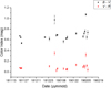 |
Fig. 7 Color variation in 64P over the observations with date. The two anomalous points indicating redder color in B – V and V – R are from the data of January 1, 2019, and February 5, 2019. |
4.3 The anomalous color
The anomalously blue color of 64P could be the result of a long-term variation event. With our multiwavelength data in Fig. 7 we show the change in color of 64P over all the observations. Most of the B – V falls in the range of 0.6–0.8 and V – R falls in the range of 0.0−0.2 mag; however, there were two days when the color changed abruptly and significantly. One day was January 1, 2019; the other day was February 5, 2019. The amplitude of the abrupt change reached 0.5 for B − R, and the timescales of these two events were constrained to one or two days because the previous and the next observation date did not show a similar result or possible trend to explain such an anomaly. We note that the outburst mentioned above took place on around January 3, 2019, just after the temporary change of B – R index on January 1, 2019. The color index during the observed outburst remained basically the same during most of our observations, suggesting typical dust particle composition or distribution. It is suspicious that the color anomaly on January 1, 2019, could be related to the outburst, but no outburst was recorded, despite available observations on consecutive days around the other anomaly. It is also unclear, due to the lack of our data and the short timescale of such anomaly, if this anomaly occurs periodically. Ivanova et al. (2017) also observed a similar event on comet C/2013 UQ4 (Catalina). They reported B – R = 0.90 ± 0.11 on July 16, 2014, and B – R = 1.41 ± 0.14 on July 18, 2014, meaning that the color of this comet also experienced significant variation on a rather short timescale. They interpreted this anomaly using dust grain models of different compositions, and concluded that the heterogeneous composition of the comet was the main reason for this anomaly. In Sect. 4.4, we present another approach to investigating the dependency between color and the aperture to find more clues to this anomalous color.
The consistent relatively small V – R index of 64P shows a bluer color than most of the comets and the Sun, while no previous record of the color of this comet can be found for comparison. One possibility is that 64P could preserve primitive materials within its nucleus, and we were observing the release of these materials. However, this phenomenon would cause the comet to be rather active, while the A(0)fρ value of 64P (see Sect. 3.2) does not seem prominent among the JFCs. Though the typical color of comets turns out to be redder than the Sun, several snapshot color measurements of different comets were reported showing blue color (Korsun et al. 2010; Zubko et al. 2014). As for long timescale variation, a similar bluing phenomenon was recorded recently on the comet C/2019 Y4 (ATLAS) before its splitting event, indicating a large amount of gas released (Hui & Ye 2020; Ye et al. 2021). Compared to the previous examples, the minimum V – R color of our observation for 64P lasted over 100 days, exceeding other bluing events recorded, and the tendency of gradual change is not recognized. Notably from August to September 2018, three months before our observations, the reported color converted to BVRI system was V – R = 0.30 ± 0.02 (Kelley et al. 2019). This result is redder than ours, and it matches our expectation for JFCs, suggesting that 64P underwent a bluing process between September and November in 2018. The deviations from the mean color of comets might be indicative of unusual phenomena presented by an active comet, or a change in grain size distribution and/or composition, as Betzler et al. (2020) suggested. In particular, Ivanova et al. (2017) pointed out that the color of magnesium-rich silicate is consistent with the blue color we observed. Cremonese et al. (2016) showed that 16 of 70 dust grains ejected from 67P presented blue color, indicating that recent activity in different heterogeneous regions could create color variations. In addition, the blue color observed on comets could be produced by hydrated minerals or even tiny water ice particles. However, due to the limitation of our data resources, the main cause for a minimum V – R color of 64P is still mysterious to us.
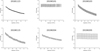 |
Fig. 8 Aperture size dependence of color shown for different dates of our observations. We spotted a general trend that the coma becomes bluer with larger aperture used. This trend does not apply on the two days with unusual color (January 1, 2019, and February 5, 2019). |
4.4 Color-aperture dependency
The dependency between color and the aperture size used for photometry has been investigated by many other researches (Li et al. 2013; Betzler et al. 2017; Kolokolova et al. 2003). We measured the color variation in the dust coma of 64P between 3000 km and 10 000 km from the nucleus; selected results are plotted in Fig. 8. We found a general trend in our observations that while we enlarge the aperture size, the color gets bluer. For most of our observations, the slope of the color-aperture diagram varies in the range from −0.2 mag/10 000 km to −0.3 mag/10 000km, and the mean value is −0.26 ± 0.04mag/10000km. This phenomenon can be explained by the particle size sorting effect (Fink & Rubin 2012). This effect means that different sizes of dust particles occupy different positions in the coma. The motion of dust particles outside the innermost coma is basically controlled by their terminal velocity, the Sun’s gravity, and radiation pressure (Fulle et al. 2010). For relatively large particles, the terminal velocity is smaller and the radiation pressure is negligible, and thus they concentrate near the center of the coma. Lighter particles have higher terminal velocity and are more sensitive to the radiation pressure, so they move to the outer part of the coma. If we assume all these dust particles have similar compositions, then the larger dust particles will appear redder (Kolokolova et al. 2001). In this case the center of the coma will have be redder than the outer part, which is consistent with our observation. It also implies that for most cases the color measured for the coma could vary with the aperture used for photometric analysis.
On January 1 and February 5, 2019, we recorded zero slope in the color-aperture diagram, shown in Fig. 8. The color remained unchanged regardless of the aperture size. Remarkably, the anomaly sighted on these two days coincides with the abrupt change in coma color we previously mentioned. Combining the results above, we can conclude that on January 1 and February 5, 2019, the daily variation in the coma color reddened about 0.5 mag on B – R color on the basis of a 6000 km aperture. We also find that with larger aperture used for photometry, a bigger variation in color would be recorded. In these scenarios the particle size sorting effect is no longer applicable because the timescale of the variation is too short to allow large particles to diffuse into the outer coma. Our dust tail model (see Sect. 4.1) demonstrates that only small particles whose radii are less than 100 µm could have the possibility to escape to the largest aperture (15 000 km) used here within one day. Since the A(0)fρ value did not change much compared with observations on consecutive dates, a possible explanation for the abrupt change in color and color-aperture relation in the coma could be the intermittent release of redder dust particles with different compositions. Those particles could be small in size, hence they do not contribute much to the mass loss of the coma and the activity measured from photometric results.
5 Summary and conclusion
We performed secular multiwavelength broadband photometry of the JFC 64P, from 1.39 au to 1.82 au outbound in 2018 and 2019. Our aims were to research the physical properties and activity of 64P. We happened to observe an outburst on around January 3, 2019. Our main results can be summarized as follows:
For 64P, the R-band A(0) fρ was computed in an aperture of radius ρ = 6000 km, and its A(0) fρ curves are presented. The results matched the general trend that A(0) fρ increased to its peak activity after its perihelion, and then decreased with increasing rh, except for the outburst event we observed. In the outburst condition we recorded a A(0) fρ value of 334 ± 6 cm on January 3, 2019;
The dust coma morphology of 64P was investigated using an azimuthally averaged method. It shows a dust jet in the anti-solar direction. During the outburst situation, the dust jet was first strengthened, then became diffuse, and finally turned back to its usual appearance;
The surface brightness profiles of 64P show a slope of 0.92±0.05 that remains almost the same during our observations, suggesting the coma was constantly in a standard steady state, as the fountain model interpreted;
The analysis of the multiwavelength observation reveals that the mean color of 64P during our observation is B – V = 0.68 ± 0.03, V – R = 0.08 ± 0.01. Compared to other JFCs, the B – V color is similar, but the V – R color value is much smaller. It seems that the 64P could be bluer than other comets, but the cause is unknown;
The color-aperture diagram for each day of the observations suggests a particle size sorting effect for 64P that the larger dust particles occupy the inner coma, while the smaller particles dominate the outer coma;
The origin of the outburst observed on 64P could be limited, but remains uncertain. It could be volatile-driven pressure mechanisms or nonvolatile-driven mechanisms such as landslides and avalanches, or a combination of the two mechanisms.
With the observations and the modelling result presented above, we can conclude that comet 64P is quite active among the JFCs and it presented a steady-state coma after its perihelion in the 2018–2019 apparitions. However, the characterization of dust coma environment of this comet before the perihelion still requires further observations in the future apparitions. In addition, it is likely that the color anomaly may appear again under similar geometric conditions if the long-lasting blue color we observed is caused by the release of bluer dust particles.
Acknowledgements
We thank the anonymous referee for comments that improved the paper. We acknowledge the support of the B-type Strategic Priority Program of CAS (Grant No. XDB41010104), the National Natural Science Foundation of China (Grant Nos. 12173093, 12033010, 12103091 and 11633009), and the Natural Science Foundation of Jiangsu Province (BK20191512). We acknowledge the science research grants from the China Manned Space Project with No. CMS-CSST-2021-B08, the Space debris and NEO research project (Nos. KJSP2020020204, KJSP2020020205 and KJSP2020020102) and Civil Aerospace pre research project (Nos. D020304 and D020302). We acknowledge the support of the Minor Planet Foundation of Purple Mountain Observatory. This research has made use of data provided by the Yaoan High Precision Telescope. This research has made use of the scientific software at www.comet-toolbox.com (Vincent, J.-B., Comet-toolbox: numerical simulations of cometary dust tails in your browser, Asteroids Comets Meteors conference, 2014, Helsinki).
References
- Agarwal, J., Della Corte, V., Feldman, P. D., et al. 2017, MNRAS, 469, s606 [NASA ADS] [CrossRef] [Google Scholar]
- A’Hearn, M. F., Schleicher, D. G., Millis, R. L., Feldman, P. D., & Thompson, D. T. 1984, AJ, 89, 579 [Google Scholar]
- Bertini, I. 2011, Planet. Space Sci., 59, 365 [NASA ADS] [CrossRef] [Google Scholar]
- Bertini, I., La Forgia, F., Tubiana, C., et al. 2017, MNRAS, 469, S404 [NASA ADS] [CrossRef] [Google Scholar]
- Betzler, A. S., Almeida, R. S., Cerqueira, W. J., et al. 2017, Adv. Space Res., 60, 612 [NASA ADS] [CrossRef] [Google Scholar]
- Betzler, A. S., de Sousa, O. F., Diepvens, A., & Bettio, T. M. 2020, Ap&SS, 365, 102 [NASA ADS] [CrossRef] [Google Scholar]
- Birkle, K., & Boehnhardt, H. 1992, Earth Moon and Planets, 57, 191 [CrossRef] [Google Scholar]
- Blackwell, D. E., & Willstrop, R. V. 1957, MNRAS, 117, 590 [NASA ADS] [CrossRef] [Google Scholar]
- Boehnhardt, H., & Birkle, K. 1994, A&Amp;AS, 107, 101 [NASA ADS] [Google Scholar]
- Cremonese, G., Simioni, E., Ragazzoni, R., et al. 2016, A&Amp;A, 588, A59 [NASA ADS] [CrossRef] [EDP Sciences] [Google Scholar]
- Crifo, J. F. 1991, in IAU Colloq. 116: Comets in the post-Halley era, eds. J. Newburn, R. L. M. Neugebauer, & J. Rahe, Astrophysics and Space Science Library, 167, 937 [NASA ADS] [Google Scholar]
- Divine, N. 1981, in The Comet Halley. Dust and Gas Environment, eds. B. Battrick, & E. Swallow, ESA Special Publication, 174, 47 [NASA ADS] [Google Scholar]
- Ehlert, S., Moticska, N., & Egal, A. 2019, AJ, 158, 7 [NASA ADS] [CrossRef] [Google Scholar]
- Farnham, T. L. 2009, Planet. Space Sci., 57, 1192 [CrossRef] [Google Scholar]
- Fernández, J. A., Tancredi, G., Rickman, H., & Licandro, J. 1999, A&A, 352, 327 [NASA ADS] [Google Scholar]
- Fink, U., & Rubin, M. 2012, Icarus, 221, 721 [NASA ADS] [CrossRef] [Google Scholar]
- Finson, M. J., & Probstein, R. F. 1968, ApJ, 154, 327 [Google Scholar]
- Fulle, M. 1989, A&A, 217, 283 [NASA ADS] [Google Scholar]
- Fulle, M., Barbieri, C., Cremonese, G., et al. 2004, A&A, 422, 357 [NASA ADS] [CrossRef] [EDP Sciences] [Google Scholar]
- Fulle, M., Colangeli, L., Agarwal, J., et al. 2010, A&A, 522, A63 [NASA ADS] [CrossRef] [EDP Sciences] [Google Scholar]
- Gehrz, R. D., & Ney, E. P. 1992, Icarus, 100, 162 [CrossRef] [Google Scholar]
- Gronkowski, P. 2004, MNRAS, 354, 142 [CrossRef] [Google Scholar]
- Gronkowski, P., & Wesołowski, M. 2016, Earth Moon and Planets, 119, 23 [CrossRef] [Google Scholar]
- Holmberg, J., Flynn, C., & Portinari, L. 2006, MNRAS, 367, 449 [NASA ADS] [CrossRef] [Google Scholar]
- Holsapple, K. A. 1993, Annu. Rev. Earth Planet. Sci., 21, 333 [CrossRef] [Google Scholar]
- Hui, M.-T., & Ye, Q.-Z. 2020, AJ, 160, 91 [NASA ADS] [CrossRef] [Google Scholar]
- Ivanova, O., Zubko, E., Videen, G., et al. 2017, MNRAS, 469, 2695 [NASA ADS] [CrossRef] [Google Scholar]
- Jewitt, D. 1990, ApJ, 351, 277 [NASA ADS] [CrossRef] [Google Scholar]
- Jewitt, D. 2009, AJ, 137, 4296 [Google Scholar]
- Jewitt, D. 2015, AJ, 150, 201 [NASA ADS] [CrossRef] [Google Scholar]
- Jewitt, D. C., & Meech, K. J. 1987, ApJ, 317, 992 [Google Scholar]
- Johnson, R. E., Cooper, J. F., Lanzerotti, L. J., & Strazzulla, G. 1987, A&A, 187, 889 [NASA ADS] [Google Scholar]
- Kelley, M. S. P., Bodewits, D., Ye, Q., et al. 2019, RNAAS, 3, 126 [NASA ADS] [Google Scholar]
- Kelley, M. S. P., Farnham, T. L., Li, J.-Y., et al. 2021, PSJ, 2, 131 [NASA ADS] [Google Scholar]
- Knollenberg, J., Lin, Z. Y., Hviid, S. F., et al. 2016, A&A, 596, A89 [NASA ADS] [CrossRef] [EDP Sciences] [Google Scholar]
- Kolokolova, L., Jockers, K., Gustafson, B. Å. S., & Lichtenberg, G. 2001, J. Geophys. Res., 106, 10113 [NASA ADS] [CrossRef] [Google Scholar]
- Kolokolova, L., Lara, L., Schultz, R., Stuewe, J., & Tozzi, G. P. 2003, J. Quant. Spec. Radiat. Transf., 79, 861 [CrossRef] [Google Scholar]
- Korsun, P. P., Kulyk, I. V., Ivanova, O. V., et al. 2010, Icarus, 210, 916 [NASA ADS] [CrossRef] [Google Scholar]
- Lamy, P., & Toth, I. 2009, Icarus, 201, 674 [NASA ADS] [CrossRef] [Google Scholar]
- Lara, L. M., Tozzi, G. P., Boehnhardt, H., DiMartino, M., & Schulz, R. 2004, A&A, 422, 717 [NASA ADS] [CrossRef] [EDP Sciences] [Google Scholar]
- Li, J.-Y., Kelley, M. S. P., Knight, M. M., et al. 2013, ApJ, 779, L3 [NASA ADS] [CrossRef] [Google Scholar]
- Lowry, S. C., Fitzsimmons, A., Cartwright, I. M., & Williams, I. P. 1999, A&A, 349, 649 [NASA ADS] [Google Scholar]
- Lowry, S. C., Fitzsimmons, A., & Collander-Brown, S. 2003, A&A, 397, 329 [NASA ADS] [CrossRef] [EDP Sciences] [Google Scholar]
- Marboeuf, U., & Schmitt, B. 2014, Icarus, 242, 225 [NASA ADS] [CrossRef] [Google Scholar]
- Marcus, J. N. 2007, Int. Comet Q., 29, 39 [Google Scholar]
- Meech, K. J., & Svoren, J. 2004, Using Cometary Activity to Trace the Physical and Chemical Evolution of Cometary nuClei, eds. M. C. Festou, H. U. Keller, & H. A. Weaver, 317 [Google Scholar]
- Moreno, F., Lara, L. M., Muñoz, O., López-Moreno, J. J., & Molina, A. 2004, ApJ, 613, 1263 [NASA ADS] [CrossRef] [Google Scholar]
- Pajola, M., Höfner, S., Vincent, J. B., et al. 2017, Nat. Astron., 1, 0092 [NASA ADS] [CrossRef] [Google Scholar]
- Rahe, J., Donn, B., & Wurm, K. 1969, Atlas of cometary forms. Structures near the nucleus (NASA SP Greenbelt) [Google Scholar]
- Rinaldi, G., Bockelee-Morvan, D., Leyrat, C., et al. 2016, in AAS/Division for Planetary Sciences Meeting Abstracts, 48, 206.05 [NASA ADS] [Google Scholar]
- Roemer, E. 1958, PASP, 70, 272 [NASA ADS] [CrossRef] [Google Scholar]
- Rousselot, P., Korsun, P. P., Kulyk, I. V., et al. 2014, A&A, 571, A73 [NASA ADS] [CrossRef] [EDP Sciences] [Google Scholar]
- Samarasinha, N. H., & Larson, S. M. 2014, Icarus, 239, 168 [NASA ADS] [CrossRef] [Google Scholar]
- Schleicher, D. G., & Bair, A. N. 2011, AJ, 141, 177 [Google Scholar]
- Schleicher, D. G., Millis, R. L., & Birch, P. V. 1998, Icarus, 132, 397 [NASA ADS] [CrossRef] [Google Scholar]
- Shi, J., Ma, Y., Liang, H., & Xu, R. 2019, Sci. Rep., 9, 5492 [NASA ADS] [CrossRef] [Google Scholar]
- Solontoi, M., Ivezić, Ž., Jurić, M., et al. 2012, Icarus, 218, 571 [CrossRef] [Google Scholar]
- Steckloff, J., & Melosh, H. J. 2016, in AAS/Division for Planetary Sciences Meeting Abstracts, 48, 206.06 [NASA ADS] [Google Scholar]
- Tancredi, G., Fernández, J. A., Rickman, H., & Licandro, J. 2006, Icarus, 182, 527 [NASA ADS] [CrossRef] [Google Scholar]
- Tozzi, G. P., Boehnhardt, H., & Lo Curto, G. 2003, A&A, 398, L41 [NASA ADS] [CrossRef] [EDP Sciences] [Google Scholar]
- Trigo-Rodríguez, J. M., García-Melendo, E., Davidsson, B. J. R., et al. 2008, A&A, 485, 599 [NASA ADS] [CrossRef] [EDP Sciences] [Google Scholar]
- Vaghi, S. 1973, A&A, 24, 41 [NASA ADS] [Google Scholar]
- Vincent, J. 2014, in Asteroids, Comets, Meteors, eds. K. Muinonen, A. Penttilä, M. Granvik, A. Virkki, G. Fedorets, O. Wilkman, & T. Kohout, 565 [Google Scholar]
- Vincent, J. B., A’Hearn, M. F., Lin, Z. Y., et al. 2016, MNRAS, 462, S184 [NASA ADS] [CrossRef] [Google Scholar]
- Ye, Q., Jewitt, D., Hui, M.-T., et al. 2021, AJ, 162, 70 [NASA ADS] [CrossRef] [Google Scholar]
- Zubko, E., Muinonen, K., Videen, G., & Kiselev, N. N. 2014, MNRAS, 440, 2928 [NASA ADS] [CrossRef] [Google Scholar]
All Tables
All Figures
|
Fig. 1 Co-added R-band images of 64P on various imaging dates (as labeled). The Y-axes are realigned to the northern direction, and east is to the left. The field of view is approximately 1′ × 1′ for each image. The yellow arrow represents the Sun’s direction, while the blue arrow represents the velocity direction of the comet. |
| In the text | |
|
Fig. 2 A(0)fρ curve throughout the whole observations. The arrow indicates the data points apart from the fitting curve, which is an unexpected peak of estimated outburst. |
| In the text | |
|
Fig. 3 Co-added R-band images of 64P on January 1 (upper left), January 3 (upper right), January 4 (bottom left), and January 11 (bottom right), 2019. The Y-axes are realigned to the northern direction, and east is to the left. The field of view is approximately 1′ × 1′ for each image. The yellow arrow represents the Sun’s direction, while the blue arrow represents the velocity direction of the comet. |
| In the text | |
|
Fig. 4 R-band images of 64P after applying azimuthally averaged methods on January 1 (upper left), January 3 (upper right), January 4 (bottom left), and January 11 (bottom right), 2019. The Y-axes are realigned to the northern direction and east is to the left. The field of view is approximately 1′× 1′ for each image. The yellow arrow represents the Sun’s direction, while the blue arrow represents the velocity direction of the comet. |
| In the text | |
|
Fig. 5 Surface brightness profiles of 64P on January 1 (left, before outburst) and January 3 (right, after outburst), 2019, in R filter. The diagonal lines in the lower left of each panel indicate gradients m = −1 and m = −3/2 for visual reference. The linear fit is made with data between 3000 km aperture and 10 000 km aperture |
| In the text | |
|
Fig. 6 Isophote contour plot of the R-band observed coma (left) and the simulated dust coma (right) on January 1, 2019. The field of view is approximately 1′× 1′’ for each image. The contour lines correspond to 21.5, 20.8, 20.4, and 20.0 mag arcsec-2. |
| In the text | |
|
Fig. 7 Color variation in 64P over the observations with date. The two anomalous points indicating redder color in B – V and V – R are from the data of January 1, 2019, and February 5, 2019. |
| In the text | |
|
Fig. 8 Aperture size dependence of color shown for different dates of our observations. We spotted a general trend that the coma becomes bluer with larger aperture used. This trend does not apply on the two days with unusual color (January 1, 2019, and February 5, 2019). |
| In the text | |
Current usage metrics show cumulative count of Article Views (full-text article views including HTML views, PDF and ePub downloads, according to the available data) and Abstracts Views on Vision4Press platform.
Data correspond to usage on the plateform after 2015. The current usage metrics is available 48-96 hours after online publication and is updated daily on week days.
Initial download of the metrics may take a while.