| Issue |
A&A
Volume 687, July 2024
|
|
|---|---|---|
| Article Number | A297 | |
| Number of page(s) | 12 | |
| Section | Planets and planetary systems | |
| DOI | https://doi.org/10.1051/0004-6361/202449145 | |
| Published online | 24 July 2024 | |
Dust properties and their variations in comet C/2013 X1 (PANSTARRS)
1
Astronomical Institute of the Slovak Academy of Sciences,
05960
Tatranska Lomnica,
Slovak Republic
e-mail: This email address is being protected from spambots. You need JavaScript enabled to view it.
2
Planetary Atmospheres Group, Institute for Basic Science (IBS),
Daejeon
34126,
South Korea
3
Astronomical Observatory of Taras Shevchenko National University of Kyiv,
3 Observatorna St.,
Kyiv
04053,
Ukraine
4
Max Planck Institute for Solar System Research,
Justus-von-Liebig-Weg 3,
37077
Göttingen,
Germany
5
Space Science Institute,
4750 Walnut Street, Boulder Suite 205,
CO 80301,
USA
6
Department of Atmospheric Sciences, Texas A&M University,
College Station,
TX,
USA
Received:
2
January
2024
Accepted:
11
June
2024
Abstract
Context. We analyze the results of photometric monitoring of comet C/2013 X1 (PANSTARRS) from December 2015 until January 2016 obtained within B, V, and R Johnson–Cousins filters.
Aims. The main objective is to investigate the dust coma and to obtain the physical characteristics of its dust particles.
Methods. We analyzed our observations using model-agglomerated debris particles, and we constrained the microphysical properties of the dust in comet C/2013 X1 (PANSTARRS) on the pre-outburst and post-outburst epochs. Moreover, we applied a geometrical model to the images processed by digital filters to estimate the rotational period of the nucleus.
Results. Our campaign revealed a sharp increase in the comet brightness on January 1, 2016. The B − V and V − R colors calculated within an aperture size of 17 000 km appear to be mostly red, except for the outburst date. The dust production (A f ρ proxy) and normalized spectral gradient S′ (B − R) dramatically changed on January 2 as compared to what was seen in December 2015. According to this model, the C/2013 X1 coma was populated by 70% organic-matter particles by volume and by two types of silicate particles together, constituting the other 30%. One type of silicate particles was composed of Mg-rich silicates, whereas the other type was composed of both Mg-rich and Fe-poor silicates. Using the geometrical model, we estimate the nucleus rotational period to be (24.02 ± 0.02) h. We interpret the observed coma morphology by two jet structures, one structure that formed by the near-pole active area at a latitude of (85+5−3)°, and the other structure formed by an active area at a latitude of (+40 ± 5)°.
Key words: methods: numerical / methods: observational / techniques: photometric / comets: general / comets: individual: C/2013 X1
© The Authors 2024
 Open Access article, published by EDP Sciences, under the terms of the Creative Commons Attribution License (https://creativecommons.org/licenses/by/4.0), which permits unrestricted use, distribution, and reproduction in any medium, provided the original work is properly cited.
This article is published in open access under the Subscribe to Open model. This email address is being protected from spambots. You need JavaScript enabled to view it. to support open access publication.
1 Introduction
According to the currently accepted concept of the Solar System cosmogony, comets contain the least processed materials in the Solar System since the time of its formation. Long-period comets, and especially those that enter the inner part of the Solar System for the first time since its formation (also referred to as dynamically new comets), provide important clues for a better understanding of the formation of our planetary system. These comets spend most of their life in a very distant part of the Solar System, and hence, they consist of materials that were little affected by solar radiation.
The nucleus of a comet is small and is in most cases too faint to be observed at visible wavelengths using ground-based instruments because the much brighter coma obscures it. Therefore, we can study the nucleus only based on observations of dust particles and gas molecules that are emitted upon its approach to the Sun. Astronomical observations show a cumulative reflectivity of the coma at several wavelengths. When the light-scattering response is measured in the innermost coma, it mainly arises from elastic scattering of the sunlight by cometary dust particles (e.g., Luk’yanyk et al. 2020). The cumulative reflectivity is a product of their total geometric cross-section and the average reflectivity of individual particles. In general, both these characteristics are barely known for a given comet. Multiwavelength photometry provides the color of dust particles, which is the reflectivity ratio at two wavelengths. It is therefore independent of the number of dust particles.
Thus, the photometric color is determined by the microphysical properties of the dust particles that scatter the light. Its temporal and/or spatial variations in a comet can reveal changes in the dust population of its coma. These changes might be caused by dust emission from different parts of a heterogeneous nucleus. However, other mechanisms might also produce a similar effect on the color of a comet. Fragmentation is often considered to play an important role, but this can occur mainly in close proximity to the nucleus due to the small size of the dust particles. If these particles contain ice, they will in most occurrences sublimate during a very short time and might destroy or fragment dust particles with an agglomerate morphology.
It is worth noting that other nondestructive processes might also cause temporal and spatial variations in the color of a comet. Solar radiation pressure produces the strongest effect. Radiation pressure is determined from the microphysics of dust particles, such as size and chemical composition. For instance, carbonaceous submicron- and micron-sized particles experience a three-fold stronger impact of solar radiation pressure than silicate particles of the same size (Zubko et al. 2015a). This means that carbonaceous particles are swept out of the inner coma much faster than silicate particles, which would also affect the color of the inner coma. The difference in the material density of different species of cometary dust is also significant. Silicate particles, for instance, are at least two times heavier than carbonaceous particles of the same morphology. This implies that they will acquire a considerably slower motion from the expanding gases. Thus, the silicate particles will remain longer within the inner coma, and this will increase their contribution to the cumulative light-scattering response (e.g., Zubko et al. 2015a).
In this work, we report and analyze our photometric survey of the long-period comet C/2013 X1 (PANSTARRS) (hereafter C/2013 X1). This comet was discovered on December 4, 2013, by the Panoramic Survey Telescope and Rapid Response System (Pan-STARRS) 1 telescope on Mount Haleakala (Bolin et al. 2013). The comet probably did not visit the inner part of the Solar System for the first time. Manzini et al. (2016) suggested that it might be a dynamically old comet. On the other hand, Combi et al. (2018) classified C/2013 X1 as a young long-period comet based on the classification introduced by A’Hearn et al. (1995). Nevertheless, the C/2013 X1 outbound orbit has an eccentricity of 1.00101, implying that it is a hyperbolic comet that will eventually leave the Solar System. The comet passed its perihelion at 1.314 au on April 20, 2016. Our observations were made in the pre-perihelion period. The paper is organized as follows: Sec. 2 describes the observations and data reductions, Sec. 3 reports the obtained results, and Sec. 4 briefly introduces the model. Sec. 5 provides a quantitative interpretation of our observations and the corresponding discussion. We summarize our findings in the summary section.
2 Observations and data reduction
Photometrical observations of comet C/2013 X1 were performed through the B, V, and R filters of the Johnson-Cousins system at the Skalnaté Pleso Observatory (Slovakia, international code 056) from December 5, 2015, to January 8, 2016. We used the 61 cm telescope equipped with the CCD detector SBIG ST-10XME with 2184 × 1472 pixels, corresponding to 19.5′ × 13.1′ on the sky plane without binning. We binned at 3 × 3, which resulted in a resolution of 1.605″ per element. The observation nights were photometric and the seeing nearly 3.2″. The geometrical circumstances of comet C/2013 X1 during the observations are collected in Table 1.
Preliminary reductions were processed via a standard algorithm for each observed night, including bias subtraction, dark and flat-field correction, and other specified procedures. The images were also cleaned from cosmic rays. The sky level was subtracted using the standard IDL procedure. In addition, the entire series of homogeneous data per one observation night were summed for further use. For the photometric calibration of our data, we used the stars in the field of view. The stellar magnitudes of the standard stars were taken from the catalog UCAC4 (Zacharias et al. 2013), the accuracy of which is 0.05–0.1 mag.
For each date, we obtained magnitudes within an aperture sized of about 17000 km in projected radius. We used a small aperture to reduce the gaseous contribution to the measured flux. It is worth noting that the elastic light scattering from dust dominates radiation scattered from the coma up to approximately 20 000 km (Luk’yanyk et al. 2020; Zubko et al. 2020a).
Based on the apparent magnitudes of comet C/2013 X1, we computed the A f ρ parameter (A’Hearn et al. 1984). This characteristic serves as a proxy for the activity level of a nucleus and might be connected to the dust production rate of the cometary nucleus (Weaver et al. 1999). However, the dust production rate depends on further assumptions of the size of the dust particles, their geometric albedo, and on the terminal velocity upon their ejection from the nucleus.
According to (A’Hearn et al. 1984), the A f ρ parameter is a product of three characteristics: (1) the albedo A of the dust particles; (2) the filling factor f, which is the ratio of the cumulative geometric cross-section of cometary dust particles over the projected cross-section of the circular aperture measured at the location of the comet; and (3) the radius ρ of the circular aperture. Since A and f are dimensionless parameters by definition, the A f ρ parameter is measured in the same units as the radius ρ, often given in centimeters. In practice, the A f ρ parameter can be inferred from the apparent magnitude of the comet as follows (A’Hearn et al. 1984; Mazzotta Epifani et al. 2010):
![Mathematical equation: $\[{Af } \rho=\frac{4 r_{\mathrm{h}}^2 \Delta^2}{\rho} \times 10^{0.4\left(m_{\mathrm{Sun}}-m_{\mathrm{c}}\right)},\]$](/articles/aa/full_html/2024/07/aa49145-24/aa49145-24-eq2.png) (1)
(1)
where mc and mSun are the apparent magnitudes of the comet in the ground-based observations and of the Sun measured in the same spectral band (Mazzotta Epifani et al. 2010). rh and Δ in Eq. (1) correspond to the comet and are measured in au and centimeters, respectively. The aperture radius ρ is also given in centimeters.
The albedo A is a function of the phase angle α and, hence, the A f ρ parameter, is noticeably affected by the geometry of observations. However, it is important to stress that there is no standard method for retrieving the phase-angle dependence of A remotely because dust outflow from a nucleus varies significantly in time. The outflow is accompanied by short-term variations presumably caused by rotation of the nucleus and/or outburst activity, along with long-term variations invoked by the changing heliocentric distance.
The A f ρ parameter is traditionally adjusted to the exact backscattering value A(0°)f ρ using the phase function inferred by Schleicher et al. (1998) for comet 1P/Halley. However, we did not reduce the dust production value to a zero phase angle. This choice facilitates a comparison of our findings with results provided by other authors for different comets within appropriate filters.
In contrast to the A f ρ parameter, the photometric color is independent of the number density of dust particles within the coma. It is therefore much less affected by nonuniform emissions from the nucleus. The photometric color allows us to immediately address the microphysics of cometary dust. Its temporal variations, if not caused by changing phase angle (Zubko et al. 2014), provide important clues to the changes in the dust population of the coma. The color can be quantified in terms of the color slope, which is defined as follows (A’Hearn et al. 1984):
![Mathematical equation: $\[S^{\prime}=\frac{10^{0.4 \Delta m}-1}{10^{0.4 \Delta m}+1} \times \frac{20}{\lambda_2-\lambda_1},\]$](/articles/aa/full_html/2024/07/aa49145-24/aa49145-24-eq3.png) (2)
(2)
where Δm stands for the true color index of the comet, that is, the observed color reduced by the initial solar color, and λ1 and λ2 correspond to the effective wavelengths of the filters used, where λ1 < λ2. The color slope is measured in percent per 1000 Å.
Observation log of comet C/2013 X1 (PANSTARRS).
3 Photometrical results and analysis
3.1 Coma morphology
We constructed intensity maps for each observed date to analyze the coma morphology of C/2013 X1. Figure 1 shows intensity maps that demonstrate the changes in the morphological structure during the observations.
To reveal faint structures in the coma, we applied digital filters. To eliminate the appearance of artifacts, we used different enhancement techniques for the filtering. We applied digital filters to each image obtained during one night and to the coadded composite image for the same night. Then, we analyzed the processed images in detail. If the structure was absent in at least one image, we excluded it. We also used techniques based on shifting the image center when the structures changed in time, and we determined whether this structure did exist or was an artifact. Similar techniques have been widely used to detect and analyze different structures in cometary comae and have shown good results (e.g. Vincent et al. 2010; Lin et al. 2012; Tubiana et al. 2015; Rosenbush et al. 2017; Garcia et al. 2020, and references therein). The resulting images were processed by a rotational gradient method (Larson & Sekanina 1984), and the division by the azimuthally averaged profile (Samarasinha & Larson 2014) is presented in the middle and right panels for each day in Fig. 1. The images show the change in morphology over time. At the beginning of our observation set (December 5–12, 2015), the tail started not at the nucleus, but at a noticeable distance from it (approximately 40 000 km). The active jet-like structure might be assumed to have shifted the origin of the tail. An active jet can notably enhance the brightness of the coma areas over which it lies. By using a digital rotational gradient filter, these areas can be emphasized in the image without displaying background coma from neighboring regions. When the jet is oriented away from the axis connecting the comet and the Sun, the visible origin of the tail also shifts in that direction. Due to decreased jet activity, the tail shift disappeared, and the tail origin matched the optocenter located at the nucleus. During the observation period, the jet structure was visible in the coma of 2013 X1, which changed its activity while the direction varied insignificantly. This variation could be explained by the change in the locations of observer and comet due to the orbiting comet. A jet structure like this usually forms near the polar region of the nucleus, which allows it to keep the direction close to the nucleus spin axis.
To interpret the images, we applied a geometrical model (see details in Rosenbush et al. 2020; Ivanova et al. 2021). The geometrical model was formulated to track the evolution of active structures over extended periods and enables the simulation of all coma images using a single set of parameters. The model computes the positions of sets of three particles that are simultaneously ejected from the nucleus at identical velocities, thereby determining the width of the ejection cone. As time progresses, the cometary nucleus rotates, and the next set of three particles escapes in slightly altered directions. By calculating the positions of these simultaneously ejected particles, we establish the visible cross-section of the active structure when projected onto the celestial plane. The image of the active structure comprises a collection of these sections for particles that are released at different times. At each moment of time, the position of the model particles and their velocities are known. This allows us to calculate the new position of the model particles for a new observation date and enables monitoring temporal changes in the configuration of active structures. Particle emissions occur when the Sun illuminates the nucleus, accounting for any potential time delay. This delay incorporates the time needed for the surface to warm up sufficiently for active gas and dust release to commence. When the Sun sets over the active zone, the particle emissions cease. The model can also adjust a time delay in particle emission cessation post-sunset due to thermal inertia. Neglecting solar radiation acceleration imposes a constraint on the particle movement time and, consequently, on the distance from the nucleus, where the deviation from a steady motion trajectory becomes significant. By limiting the maximum permissible deviation to Δρ/ρ = 0.05 and considering particles with radiation pressure parameter β < 0.01, we can estimate the maximum permitted distance ρmax = 40 000 km for the model application. The geometrical model allows us to determine the form of a jet-like structure projected on the sky plane, considering the positions of the Earth, the Sun, and the comet nucleus. The initial parameters of the model are the rotational period of the nucleus, the spin-axis position, and the coordinates of the active areas that form jet structures on the nucleus surface. The model parameters are calculated to align the images of model jets with the observed active structures. Since this model is dynamic, it is computed for all observation dates, and the alignment of images across all dates with a single set of parameters is verified. Having multiple observations over time reduces potential ambiguities in interpreting the active structure patterns and enhances the accuracy of the parameter determination. The accuracy of these parameters is assessed by varying one parameter while keeping the others constant.
Using the geometrical model, we interpreted the observed coma morphology by two jet-like structures (Fig. 2). We included the observation from the 6m telescope obtained with the broadband g–SDSS filter on November 4, 2015, in our modeling, when the comet was 2.658 au from the Sun (Shubina et al. 2024) to have a more comprehensive data range. Our modeling revealed the following. One of the structures, indicated as J1, was formed by a near-pole active area at a latitude of ![Mathematical equation: $\[\left(85_{+5}^{-3}\right)^{\circ}\]$](/articles/aa/full_html/2024/07/aa49145-24/aa49145-24-eq4.png) , and the other structure, J2, is an active area at a latitude of (+40 ± 5)°. Favorable conditions for jet-like structure formation can appear in the polar regions, particularly when there are noticeable deviations from an angle of 90° between the heliocentric radius vector and the cometary rotation axis. This deviation results in the polar summer effect, where the Sun continuously illuminates the polar zone. Furthermore, straight jets are formed in the circumpolar region. In this case, however, the position angle of the jet remains unchanged while the nucleus rotates (see, for instance, Manzini et al. 2021; Oldani et al. 2023). The velocity of particles in structure J2 was determined from its form and is estimated at 0.44 ± 0.07 km s−1. Table 2 lists the position angles of the revealed active structures shown in Fig. 2. Figure 2 and Table 2 show that the position angle of these active structures changed significantly from November to December 2015. However, the values were stabel within error bars from December to January.
, and the other structure, J2, is an active area at a latitude of (+40 ± 5)°. Favorable conditions for jet-like structure formation can appear in the polar regions, particularly when there are noticeable deviations from an angle of 90° between the heliocentric radius vector and the cometary rotation axis. This deviation results in the polar summer effect, where the Sun continuously illuminates the polar zone. Furthermore, straight jets are formed in the circumpolar region. In this case, however, the position angle of the jet remains unchanged while the nucleus rotates (see, for instance, Manzini et al. 2021; Oldani et al. 2023). The velocity of particles in structure J2 was determined from its form and is estimated at 0.44 ± 0.07 km s−1. Table 2 lists the position angles of the revealed active structures shown in Fig. 2. Figure 2 and Table 2 show that the position angle of these active structures changed significantly from November to December 2015. However, the values were stabel within error bars from December to January.
The calculated values of the nucleus spin axis are 206 ± 6° and +40 ± 4° in the north pole coordinates for the right ascension and declination, respectively. During the observations, J2 weakened and overlapped with J1. Possible reasons for the weakening or cessation of activity in the region that forms structure J2 include a local depletion of volatile substances, the formation of a mineral crust that sealed in the volatiles, or the collapse of surface features that can block the release of these substances. Additionally, the jet could cease to operate if the region moved into shadow due to the orbital movement of the comet. However, this reason does not apply in our case, given the calculated orientation of the rotation axis and the latitude of the jet formation region. When we assume that J2 was active during the whole period because of the overlap with J1 due to the projection on the sky plane, then the rotation period is 24.02 ± 0.02 h. However, considering December 12 as the last day of J2 activity, the nucleus rotational period is 24.00 ± 0.04 h. From our standpoint, the former estimation is more probable because J2 was very active in the first half of the observation set and likely continued to exist after December 12 in the less active phase. We assume this because the illumination conditions of the active area, which formed this jet structure, did not significantly change (see Fig. 3). The lasting observation set causes the precision of our rotational period estimation.
The rotational period and spin axis position of the nucleus were also determined by Manzini et al. (2016). The latter was RA = 240 ± 10° and δ = +00 ± 10°. Our findings of the right ascension are close to theirs, but the calculated rotational period and the north pole declination are not.
Manzini et al. (2016) obtained a nucleus rotational period of 11.952 ± 0.360 h for comet C/2013 X1 from a photometrical analysis. Based on our calculations, it should be twice longer. The difference between these two estimates can be explained as follows. We performed model calculations to demonstrate the potential issue of selecting half the actual rotation period using the photometric method, particularly in cases where two photometric peaks are present during the nucleus rotation. In our scenario, these two peaks correspond to two active regions on the nucleus, each forming a jet-like structure. To validate this, we simulated a model signal with a slight brightness increase (ΔI/I < 0.1) and two peaks over a period matching the nucleus rotation period. To closely mimic the conditions used in previous photometric assessments (Manzini et al. 2016) in our calculations, we generated a set of seven periods, each comprising 256 samples. We then added normally distributed noise to this dataset, with the noise parameters and magnitude change amplitude chosen based on photometric studies of the inner cometary coma (Manzini et al. 2016). We note the similarity between the photometric representations of our model signal with those of Manzini et al. (2016) when plotted on a scale equal to half the period (see Fig. 7, Manzini et al. 2016). The model sample with the half period is shown in Fig. 4.
Then, we applied a Fourier transformation to the model sample to estimate the power spectrum. The result is shown in Fig. 5. It demonstrates that for a given model signal, a value corresponding to half a period is the dominant frequency. We compared our computations with the periodogram for all photometric measurements (see Fig. 8 from Manzini et al. 2016), which shows a similar situation, in which a frequency with a period of 24 h is also present, but a frequency with a half period of about 12 h prevails. Based on our investigation, we found that the period value reported by Manzini et al. (2016) needs to be doubled. Consequently, the estimated period becomes 23.90 ± 0.72 h. This aligns closely with our estimate of 24.02 ± 0.02 h.
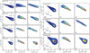 |
Fig. 1 Intensity maps of comet C/2013 X1 (PANSARRS) obtained at the Skalnaté Pleso observatory in the R filter from December 2015 to January 2016 (the dates are indicated in the left panels for each day). The left panels show direct images of the comet. The center panels show the operation of digital filters using the rotational gradient method (Larson & Sekanina 1984). The right panels show the results divided by the averaged profile (Samarasinha & Larson 2014). North, east, the Sun, and the cometary motion are indicated. |
Position angles of the revealed active structures in the coma of comet C/2013 X1 (PANSTARRS).
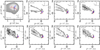 |
Fig. 2 Jet structure positions calculated from the geometrical modeling of the observed images of comet C/2013 X1 (PANSARRS) processed by the digital filters. Blue indicates jet structure J1, and red shows J2. The scale of the first image is different for clarity. |
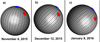 |
Fig. 3 View from the Sun side on the location of active areas corresponding to jet structures J1 (blue) and J2 (red) on the nucleus of comet C/2013 X1 (PANSTARRS). |
3.2 Dust production and colors
We estimated the dust production using the A f ρ proxy (Eq. (1)). In our calculations, we used the apparent Sun magnitudes and colors from Willmer (2018). The resulting dust production for the B, V, and R filters are listed in Table 3. All calculations were performed within an aperture radius of 17 000 km. This aperture size was chosen to cover the part of the coma where the dust component dominates, and the gas contributes less to the total flux than the dust (Zubko et al. 2020a). Moreover, Shubina et al. (2024) calculated the gas contribution based on spectral observations obtained on November 4, 2015. It was 3.8%, 7.9%, and ~9% for the R, V, and B filters, respectively. Thus, the filters transmitted a small portion of the emission radiation. However, the R filter is less contaminated by the gas emissions. As previously shown (Luk’yanyk et al. 2019; Rosenbush et al. 2017), these estimated values of the gas contribution could be neglected. Moreover, gas contributes little to the light scattering near the nucleus (Jewitt et al. 1982; Picazzio et al. 2019). Hence, our calculations are reasonable for characterizing the dust environment in the coma of comet C/2013 X1.
Figure 6 demonstrates the variation in the A f ρ parameters from December 2015 through January 2016. This plot shows an abrupt increase in the dust productivity on January 2, 2016. An outburst typically causes a sharp increase in brightness. Our assumption about the outburst agrees with the data from the COBS database1. Considering the dust production within different filters, we found that during this outburst, the dust production in the B filter is higher than in the R filter. The results from other days do not show this effect.
Table 3 also contains apparent magnitudes in the R filter, colors B − V and V − R, and color slope S′(B − R). Compared to the Sun values taken from Willmer (2018), our results are redder, except for measurements obtained during the outburst on January 2, 2016 (Fig. 7). In the two-color diagram (right panel of Fig. 7), we plot average colors for long-period comets (Meech et al. 2009) and short-period comets (Hainaut & Delsanti 2002). Our measurements of the V − R color are typical for long-period comets within the error bars, and the B − V color correlates quite well. The colors obtained during the outburst are an anomaly. Studies of the color in various comets often reveal a red color (e.g., Jewitt & Meech 1986; Kulyk et al. 2018), implying positive values of the color slope S′ > 0. However, negative values of the color slope S′ (i.e., a blue color) have also been registered in comets (e.g., Lamy et al. 2011; Zubko et al. 2014; Ivanova et al. 2017; Luk’yanyk et al. 2019, 2020) or in centaurs (Seccull et al. 2019). In the latter case, a very blue dust color of the coma of 174P/Echeclus was reported that is linked to the composition of the dust.
Table 3 and Fig. 8 summarize the results we obtained for comet C/2013 X1. The photometric color of comet C/2013 X1 varied noticeably with time. Furthermore, during only two days, from December 31, 2015, until January 2, 2016, the color of comet C/2013 X1 changed from red with S′ = (5.68 ± 1.51)% per 1000 Å to blue with S′ = −(5.89 ± 0.85)% per 1000 Å. This transition was accompanied by brightness that was more than twice higher. Five days later, on January 7, the color of comet C/2013 X1 returned to what it was on December 31. Nevertheless, its brightness did not degrade to what was observed on December 31.
Fast and dramatic changes in the photometric color have previously been observed in different comets. For instance, dramatic variations were found in comet 21P/Giacobini-Zinner when its color slope changed from S′ = 8.4% per 1000 Å to −14.9% per 1000 Å from November 24 to 25, 1998 (Lara et al. 2003). A follow-up observation on December 7 revealed a value of 23.3% per 1000 Å. Lara et al. (2003) noted that their measurements had no clear connection with gas activity, which steadily decreased from November 8 to December 8, 1998. Comet 21P/Giacobini-Zinner is classified as strongly depleted in both C2 and C3 while demonstrating strong molecular emission of CN (Cochran et al. 2015). Comet 21P/Giacobini-Zinner also has revealed noticeable variations in its positive polarization (Chornaya et al. 2020).
A similar trend in the color slope (i.e., a positive-negative-positive value) was also found in the centaur 29P/Schwassmann–Wachmann 1 in October 2018 (Voitko et al. 2022), where S′ decreased from about 10% per 1000 Å to −7% per 1000 Å and then increased to 4% per 1000 Å during 10 days. This time period should be considered quite short for 29P/Schwassmann–Wachmann 1 as it is located relatively far from the Sun, ~6 au, as the gas outflow velocity, and accordingly, the terminal velocity of dust particles accelerated by expanding gas that quickly decreases with increasing heliocentric distance. Voitko et al. (2022) also reported color-slope variations in August 2018, but the color slope did not change sign at that time. Based on the analysis of their observational results, the authors suggested that color variations are likely caused by outburst activity.
Short-term variations from −4% to almost 19% per 1000 Å during only two days were detected in comet C/2013 UQ4 (Catalina) (Ivanova et al. 2017). The authors explained this phenomenon via the chemical heterogeneity of the dust population of the coma. Similar color-slope variations, but without a change in sign, have also been reported by Hui et al. (2019) for comet C/2010 U3 (Boattini). The authors noted the connection between color changes and the crystallization of amorphous water ice during the approach of the comet to the Sun.
Another example of a dramatic color slope change from −10.15% to 16.48% per 1000 Å during one day is comet 41P/Tuttle-Giacobini-Kresak (Luk’yanyk et al. 2019). Lukyanyk et al. interpreted the variations as resulting from a change in the dust composition of a mixture of at least two end-members, Mg silicates, and organics and Mg-Fe silicates. The authors also assumed that fast and significant dust color changes might not be a unique characteristic of the comet.
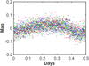 |
Fig. 4 Model signal sampled over a half-period interval with normally distributed superimposed noise. A separate color is used to indicate the model signal of each period. |
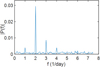 |
Fig. 5 Power spectrum of the model signal with normally distributed noise for a total duration of the model spectrum of seven periods. |
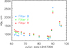 |
Fig. 6 Variation in the A f ρ parameter within the B, V, and R filters in December 2015 and January 2016. |
Photometrical parameters of comet C/203 X1 (PANSTARRS) including apparent magnitudes in R filter, colors, color slope, and A f ρ values obtained within an aperture size of ~17 000 km.
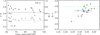 |
Fig. 7 Colors of comet C/2013 X1 (PANSTARRS). Left panel: color variation of the cometary coma in December 2015 and January 2016. The filled circles correspond to B − V and the open circles to V − R. The values for the Sun colors are represented by the solid and dashed lines, respectively. Right panel: color diagram B − V vs. V − R for comet C/2013 X1. The red star marks the color of the Sun. The blue diamond and green square indicate the mean value of the colors for long-period (Meech et al. 2009) and short-period (Hainaut & Delsanti 2002) comets. |
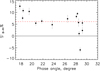 |
Fig. 8 Variations in the color slope of comet C/2013 X1 (PANSTARRS) as a function of phase angle in December 2015 and January 2016. The dashed red line indicates the mean value of the color slope, S′(B − R) = 6.08% per 1000 Å. |
4 Modeling color and polarization
We retrieved the microphysical properties of the dust population in the coma of C/2013 X1 using the model of agglomerated debris particles. These particles have demonstrated a capability to fit the degree of linear polarization (e.g., Chornaya et al. 2023; Kochergin et al. 2021; Zubko et al. 2016), photometric color, including its fast variations (Ivanova et al. 2017; Picazzio et al. 2019; Luk’yanyk et al. 2019, 2020; Voitko et al. 2022), and simultaneous polarimetric and photometric measurements of different comets (Chornaya et al. 2020; Zubko et al. 2014, 2015a). This approach is based on the results of the investigation of comets with spacecraft. In particular, it adapts the in situ findings of Mg-rich silicate particles and carbonaceous particles in cometary coma (e.g., Fomenkova et al. 1992), the morphology of micron-sized dust particles (e.g., Hörz et al. 2006), and their power-law size distribution (e.g., Mazets et al. 1986; Price et al. 2010). For a more detailed model outline, we refer to Zubko et al. (2014, 2015a, 2016). Similar methods or techniques are used widely to reproduce the dust particle parameters (e.g. Das et al. 2011; Halder & Ganesh 2021; Lasue et al. 2009).
The temporal variations in the color in comet C/2013 X1 summarized in Table 3 do not exceed what was previously reported by Ivanova et al. (2017) of comet C/2013 UQ4 (Catalina), by Luk’yanyk et al. (2019, 2020) of comet 41P/Tuttle–Giacobini–Kresák, and by Voitko et al. (2022) of the centaur 29P/Schwassmann–Wachmann 1. A two-component model, which includes two different types of dust, one of which typically is a highly absorbing representative of processed organics, and the other is refractory, typically representative of Mg-rich silicates, has demonstrated the capability of reproducing all these observations, and we expect that it could be used to model the photometric observations of comet C/2013 X1 as well.
Comet C/2013 X1 is exceptional because this comet was also observed using polarimetry. Although these observations have not been published previously, the result underwent a preliminary examination and was included in the Database of Comet Polarimetry V2.0 (Kiselev et al. 2017) (hereafter, DBCP V2.0). We incorporate them into the current analysis to further constrain the retrieval of the microphysics of dust in comet C/2013 X1. As demonstrated below, it leads to a crucially important conclusion on the chemical composition of dust in comet C/2013 X1.
According to the DBCP V2.0, at least two polarimetric observations of comet C/2013 X1 were made, on November 13, 2015, and on January 13, 2016. In the former case, the comet was observed at a phase angle of α = 10.08° through a circular aperture with a radius of ρ ≈ 17 850 km, and in the latter case, it was seen at α = 29.11° with ρ ≈ 21 550 km. The first polarimetric observation was performed approximately three weeks before the start of our campaign, and the second observation was made five days after its end. This closeness suggests that the two observation sets might correspond to the same activity state of C/2013 X1. It is worth noting that both datasets were obtained using nearly the same aperture size. We therefore developed a model that simultaneously fit the photometric color and polarization measured in comet C/2013 X1.
The two-component model is based on the model of the agglomerated debris particles. This type of irregularly shaped particle was introduced for a realistic modeling of light scattering by terrestrial and cometary dust particles (e.g. Zubko et al. 2012, 2013). We refer to Zubko et al. (2013) for a detailed description of the generation algorithm. The algorithm produces a highly irregular shape with a fluffy internal morphology. On average, the constituent material occupies only about 23.6% of the volume in the sphere that is circumscribed by the agglomerated debris particles. When we take the material density of the most abundant refractory species in comets (silicates with 3.5 g cm−3 and carbonaceous materials with ~1.5 g cm−3) into account, the bulk material density of the agglomerated debris particles falls in the range between 0.35 g cm−3 and 0.83 g cm−3. This appears to agree with the lower part of the range 0.3–3 g cm−3 found in situ in the micron-sized dust particles that were sampled in the vicinity of the 81P/Wild 2 nucleus by Stardust (Hörz et al. 2006). Moreover, the interplanetary dust particles (IDPs) collected in the Earth’s stratosphere reveal a bimodal size distribution with a peak at ~0.6 g cm−3 (Flynn & Sutton 1991), which matches the median bulk material density in the agglomerated debris particles remarkably well. IDPs presumably have a cometary origin (Nesvorný et al. 2010).
The irregular shapes and sizes comparable to the wavelength of incident electromagnetic radiation necessarily require a rigorous consideration of light scattering by agglomerated debris particles. We performed computations using the discrete dipole approximation (DDA), a numerical technique that places minimum limitations on the shape and morphology of the target particles (e.g. Draine & Goodman 1993). In practice, however, this flexibility is very expensive computationally. We generated the agglomerated debris particles in spherical initial matrices with one of two diameters: 64 cells (consisting of 137 376 cells), or 128 cells (1 099 136 cells). The choice of the initial matrix size was governed by the ratio of its radius r to the wavelength λ. The literature quantifies this ratio through the size parameter x = 2πr/λ. We used the smaller initial matrix when x < 16 and the larger matrix otherwise. On average, the agglomerated debris particles generated in the former case are composed of 32 421 cells. In the latter case, this number is larger by a factor of ~8, yielding 259 396 cells. The upper limit of the size parameter in our modeling was set to x = 32, which was demonstrated to be more than sufficient to model the light scattering by comets under any reasonable assumption of the size distribution of the dust particles that populate their comae (Zubko et al. 2020c).
For each pair of the size parameter x and the complex refractive index m, we repeated the DDA computations for a minimum of 500 randomly generated samples of the agglomerated debris particles, which guarantees statistically reliable results upon averaging over the particle shape. In addition, all computations were repeated for two wavelengths that closely matched the effective wavelength in the B and R filters. The database that we currently exploit was accumulated since 2008, and it currently includes more than 40 refractive indices computed over a wide range of the size parameter x at two wavelengths. However, these long-lasting computational efforts are worth it because modeling the light-scattering response in comets and other natural objects yields very robust results. In practice, we almost never met a nonreproducible observation of comets.
The satisfactory fit of astronomical observations of a comet by a model does not immediately guarantee an accurate retrieval of the microphysics of its dust. In order to ensure the performance of the model, it has to be verified in laboratory optical measurement. It is significant that the model of agglomerated debris particles underwent this verification in several analogs of cosmic dust, including feldspar particles (Zubko et al. 2013), forsterite particles (Zubko 2015), and olivine particles (Videen et al. 2018). A principal difference between optical experiments and astronomical observations is that the object of interest can be comprehensively, if not fully, characterized under laboratory conditions. In particular, a high level of purification of the chemical composition can be achieved, and the actual refractive index of the target particles can be obtained. Furthermore, their size distribution can be accurately measured with either a laser light-scattering technique (Martín et al. 2020), Q-space analysis (Sorensen et al. 2017), digital holographic imaging (Berg & Videen 2011), or directly from SEM images of sample particles deposited on a substrate. Last but not least, in an optical experiment, not only the intensity and degree of linear polarization of the scattered light accessible in astronomical observations can be measured, but the entire set of Mueller-matrix elements. This fully characterizes the light-scattering response (e.g. Muñoz et al. 2012). The agglomerated debris particles have demonstrated this capability when they fit the laboratory optical measurements. Their size distribution and refractive index closely match the microphysical characteristics of the target particles (Zubko et al. 2013; Zubko 2015; Videen et al. 2018). This feature increases the reliability of retrievals obtained with the agglomerated debris particles. Interestingly, these particles also helped to reconcile ground-based polarimetric observations of comet 81P/Wild 2 with in situ findings in the micron-sized dust particles sampled by the Stardust in the vicinity of the same comet (Zubko et al. 2012).
Agglomerated debris particles have been exploited so far in the modeling of astronomical observations of numerous comets, including the polarimetry of comets C/1975 V1 (West) (Zubko et al. 2014), C/1975 N1 (Kobayashi-Berger-Milon), 23P/Brorsen–Metcalf, C/1989 X1 (Austin), C/1995 O1 (Hale–Bopp), C/1996B2(Hyakutake) (Zubko et al. 2016), C/2018 V1 (Machholz–Fujikawa–Iwamoto) (Zubko et al. 2020b), C/2019 Y4 (ATLAS) Zubko et al. (2020c), 29P/ Schwassmann–Wachmann 1 Kochergin et al. (2021), C/2020 S3 (Erasmus) (Chornaya et al. 2023); by means of multi-wavelength photometry of comets C/2013 UQ4 (Catalina) (Ivanova et al. 2017), 29P/Schwassmann–Wachmann 1 (Picazzio et al. 2019; Voitko et al. 2022), 41P/Tuttle-Giacobini-Kresák (Luk’yanyk et al. 2019, 2020); and by means of both photometry and polarimetry, of comets C/2012 S1 (ISON) (Zubko et al. 2015a) and 21P/Giacobini-Zinner (Chornaya et al. 2020). Surprisingly, the microphysics of dust inferred in this variety of comets appears to agree qualitatively well with each other. The difference in light-scattering properties of these comets primarily arises from different relative abundances of Mg-rich silicate particles and carbonaceous dust particles. We considered these findings in our current analysis of photometric and polarimetric observations of comet C/2013 X1 (PanSTARRS).
Using the two-component model, we started our analysis by searching for the best fit for the polarimetric observations. The top panel in Fig. 9 demonstrates the degree of linear polarization as a function of the agglomerated debris particles with five different values of the complex refractive index m. The four curves with the real part of the refractive index Re(m) = 1.6 and imaginary parts of refractive index Im(m) = 0.0005–0.03 are representative of Mg-rich and Mg–Fe silicates with a different iron content (Dorschner et al. 1995). The refractive index m = 1.957 + 0.341i corresponds to organic matter in red light (Jenniskens 1993). In all these cases, the radius of the agglomerated debris particles spans the range from r ≈ 0.07 μm up to 2.24 μm. The light-scattering response was averaged over the given range of radius r, using the power-law size distribution r−n with index n = 2.3. This range in r is more than sufficient to reproduce the light-scattering response in comets that are observed at small phase angles (Zubko et al. 2020b).
As demonstrated in the bottom panel of Fig. 9, a mixture of the agglomerated debris particles composed of organic matter with the agglomerated debris particles with one of four silicate compositions can satisfactorily fit the polarization of light scattered by comet C/2013 X1. At Im(m) = 0.0005, which virtually matches what was measured experimentally in the pure Mg silicates (Dorschner et al. 1995), the observations are closely reproduced with a mixture of 28.5% (by volume) silicate particles and 71.5% organic-matter particles. Increasing Im(m) to 0.01 conforms with a small growth of the iron content in the Mg-rich silicates, and it yields a best fit with 37% silicate particles and 63% organic-matter particles. A further increase of the material absorption (i.e., iron content) in silicates requires a larger volume fraction in the mixture to fit the observations. It is significant that the quality of the fit of the negative polarization remains nearly the same at all levels of Im(m) of the silicate component investigated in Fig. 9. This results from the relatively weak dependence of the negative-polarization amplitude on the material absorption in the domain Im(m) = 0–0.03 (Zubko et al. 2015b). However, the volume fraction of the silicate particles grows with Im(m), which is caused by a decrease in their reflectivity.
The fits shown in the bottom panel of Fig. 9 could be improved further by adjusting the volume ratio of the two components for each of the polarimetric observations. This modeling assumes that the volume ratios are different at each epoch. For instance, a mixture of 33% silicate particles (m = 1.6 + 0.0005i) and 67% organic-matter particles (m = 1.957 + 0.341i) can exactly reproduce the polarization observed at α = 10.08°. Similarly, the polarization at α = 29.11° can be exactly matched with a mixture of 24% silicate particles and 76% organic-matter particles. However, these small deviations are insufficient to reproduce the significant variations of the photometric color found in our observational campaign.
This is evident from Fig. 10, which shows the color slope S′ as a function of phase angle α that emerges from a mixture of 28.5% silicate particles with Im(m) = 0.0005 and 71.5% organic-matter particles (shown in the left column) and from a mixture of 37% silicate particles with Im(m) = 0. 01 and 63% organic-matter particles (shown in the right column). Following the laboratory measurements by Jenniskens (1993), we set the refractive index of the organic-matter particles to m = 1.957 + 0.341i in red light and to m = 1.855 + 0.45i in blue light. This holds everywhere in Fig. 10, where the result for pure organic-matter particles is shown with the solid brown line.
The refractive index of the silicate particles in red light is set to m = 1.6 + 0. 0005i in the left panels of Fig. 10 and to m = 1.6 + 0.01i in the right panels of Fig. 10. However, different rows correspond to a different increment of the imaginary part of the refractive index ΔIm(m) in blue light. The uppermost row shows results obtained assuming no wavelength dependence of refractive index in the silicate particles, ΔIm(m) = 0. In the middle row, we assume a small excess of the material absorption in blue light, ΔIm(m) = 0.01, and in the bottom row, we show results obtained at a stronger wavelength dependence, ΔIm(m) = 0.02. Except for pure Mg silicate and water ice, virtually all well-known and plausible species of cometary dust reveal an excess of their Im(m) in blue light (see discussion in Zubko et al. 2015a). While slight nonsystematic changes in Re(m) with wavelength in the visible are possible, they do not make a noticeable effect on the light-scattering response (e.g., Fig. 7 of Zubko et al. 2014) and, hence, for the silicate particles we set Re(m) to 1.6.
The color slope in the mixture of silicate and organic-matter particles is shown in all panels of Fig. 10 with the solid magenta lines. Of the six panels of Fig. 10, only the two-component mixture that includes the pure Mg silicate particles (m = 1.6 + 0.0005i and ΔIm(m) = 0) can be potentially consistent with the entire range of the color slope observed in comet C/2013 X1. This case is shown in the top left panel. Then, the bluest color of comet C/2013 X1 would imply that its coma is predominantly populated by pure Mg silicate particles, and the reddest color would reveal the fully organic-matter composition. However, these variations necessarily suggest dramatic variations in the negative polarization of comet C/2013 X1. For instance, all our observations revealing S′ > 4.5% per 1000 Å would simultaneously imply no negative polarization in comet C/2013 X1. This behavior is hardly consistent with the results of polarimetric observations of the comet. Even though two observations are divided in time by two months, they reveal a very similar chemical composition of the C/2013 X1 coma. Therefore, the two-component approach would probably not be consistent with the two sets of observational results. It therefore requires further refinement.
This goal could be achieved by involving three components in modeling light-scattering by comet C/2013 X1. One component should be organic-matter particles because they play a crucial role in shaping the phase dependence of the degree of linear polarization in comets (Zubko et al. 2016) and, hence, in C/2013 X1. We label this component “org”.
Another component necessarily has to be the pure Mg silicate particles with m = 1.6 + 0. 0005i in blue and red light, because only these particles could match the photometric color S′ = −(5.89 ± 0.85)% per 1000 Å observed in comet C/2013 X1 on January 2, 2016. We label this component “sil1”.
The last component can correspond to the particles composed of Mg-rich silicate with some iron content. These particles could have a refractive index m = 1.6 + 0.01i in red light and m = 1.6 + 0.03i in blue light. We label them “sil2”. Their color slope as a function of the phase angle is shown in the bottom right panel of Fig. 10 with the blue line. These particles produce a very red color, S′ > 25% per 1000 Å at α ≤ 35°. However, this extremely red color will be dampened in the mixture by the sil1 component, which has a very blue color, and by the org component with its moderately red color. It is extremely important, however, that the sil1 component and the sil2 component produce a very similarly shaped branch of negative polarization (see top panel of Fig. 9).
We set the cumulative volume fraction of the sil1 particles and the sil2 particles to 30%; hence, the organic-matter particle volume fraction is equal to 70%. We maintained this ratio of silicates to organics, except for the case of the bluest photometric color detected in comet C/2013 X1 in our campaign, when the volume fraction of the org particles was necessarily reduced in favor of the sil1 particles. The chosen volume ratio of silicates to organics provides a reasonable fit for two polarimetric observations. Its quality is virtually the same as shown at the bottom in Fig. 9. However, varying the relative fraction of the sil1 and sil2 particles results in a wide range of the color-slope values, −2.4% per 1000 Å ≤ S′ ≤ 16.3% per 1000 Å, which could match our photometric observations.
The results of modeling the color slope in comet C/2013 X1 using the three-component approach are shown in the top panel of Fig. 11. The observation results are shown with brown points, which are not apparent because they overlap the purple diamonds, corresponding to the modeling results. Except for the outburst event, the color of comet C/2013 X1 in every epoch was fit one by one via adjusting the volume ratio of the sil1 and sil2 components to match the particular value of the color slope S′. In other words, the three-component approach matches the observations precisely. Four results of the modeling are labeled here in accordance with their chemical composition as follows (sil1; sil2; org). The modeled values of three components (sil1, sil2, and org) calculated for all observed data are listed in Table 4. As shown in Fig. 11 and Table 4, the color of comet C/2013 X1 at its outburst cannot be reproduced with a volume ratio of organic-matter particles of 70%. Their abundance is necessarily reduced in favor of the pure Mg silicate particles because only they are able to produce the blue color. However, the pure Mg silicate particles also yield a strong negative polarization.
It is extremely important that our modeling also yields a polarimetric response that can be compared with the measured polarization observed in comet C/2013 X1. This comparison is presented in the bottom panel of Fig. 11. The three-component model predicts a highly stable polarization behavior in comet C/2013 X1, except for the epoch of its bluest color. This stability results from the weak dependence of the negative polarization of the agglomerated debris particles on their imaginary part of the refractive index, also shown in Fig. 9. However, the same three-component model can simultaneously reproduce significant variations of the photometric color observed in comet C/2013 X1. Our modeling therefore demonstrates no contradiction between the two observational datasets. Finally, the temporal variations in the composition of a cometary coma were also detected using the mid-IR observations; cometary observations like this are rare, however. For instance, the monitoring of the coma of comet 1P/Halley in its 1985–1986 apparition revealed fast and dramatic changes in its 10 μm silicate feature. The coma demonstrated this feature on March 20 and 28, whereas on March 25, the 10 μm silicate feature disappeared (Gehrz & Ney 1992). The 10 μm silicate feature in comets is produced by a mixture of several types of silicates with a different structure (glass or crystalline) and a different relative abundance of Mg and Fe (e.g., Hanner & Bradley 2004). Temporal variations in this feature indicate changes in the dust population of the coma and suggest heterogeneities within the nucleus that emitted these materials.
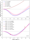 |
Fig. 9 Degree of linear polarization as a function of phase angle α. Top panel: agglomerated debris particles with five different refractive indexes (see legend) that are representative of Mg-rich silicates with a different iron content and organic matter in red light. Bottom panel: polarimetric responses measured in comet C/2013 X1 (PANSTARRS) and the four best fits obtained using the two-component model. All modeling results were obtained using polydisperse particle systems with a power-law size distribution with index n = 2.3. |
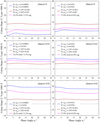 |
Fig. 10 Color slope S′(B − R) as a function of phase angle α. The left columns correspond to silicate particles of m = 1.6 + 0.0005i, and the right columns correspond to silicate particles of m = 1.6 + 0.01i in red light. The different rows correspond to a different increment of the imaginary part of refractive index ΔIm(m) in blue light ΔIm(m) = 0 (top), 0.1 (middle), and 0.2 (bottom). The organic component was set to m = 1.957 + 0.341i in red light and m = 1.855 + 0.45i in blue light everywhere. The blue and brown curves demonstrate the color slope of the Mg-rich silicate particles and organic particles, respectively. The magenta curves show the result when they are mixed. |
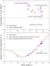 |
Fig. 11 Top panel: color slope S′(B − R) of comet C/2013 X1 (PANSTARRS) reproduced using the three-component model. For four extreme values of S′, the corresponding volume fractions of the components are given in parentheses. Bottom panel: polarimetric measurements (brown points) and predictions emerging from the three-component model of the color slope S′(B − R) (purple diamonds) of comet C/2013 X1 (PANSTARRS) together with the polarization curve of the three-component model at a constant volume ratio of the constituent components. |
Modeled volume fractions of organic-matter particles (org), Mg-poor silicates (sil1), and Mg-rich silicates (sil2) in comet C/2013 X1 (PANSTARRS).
5 Summary
We analyzed the results of observations of comet C/2013 X1 (PANSTARRS) from December 5, 2015, to January 8, 2016, in the broadband filters B, V, and R. The estimated dust production level, A f ρ proxy, in the R filter varied from 1250 ± 16 cm on December 5 to 2255 ± 22 cm and 1526 ± 32 cm on January 2 and 8. The dust production of comet C/2013 X1 appeared to be typical for other long-period comets at a similar heliocentric distance. The comet appears to have experienced an outburst on January 2, 2016. Our observations have revealed significant short-term variations in the photometric color in its coma (ρ =17 000 km). The color slope inferred with the pair of broadband B and R filters varied between S′ = (12.58 ± 1.21)% per 1000 Å detected on December 5, 2015, and S′ = −(5.89 ± 0.85)% per 1000 Å detected on January 2, 2016. Using agglomerated debris particles, we developed a three-component model capable of quantitatively reproducing the significant variations in color and the high stability in polarization observed in comet C/2013 X1 simultaneously. According to this model, the C/2013 X1 coma was populated by 70% organic-matter particles (by volume) and two types of silicate particles together, constituting another 30%. One type of silicate particles was composed of pure Mg silicates, and the other type was made of Mg-rich and Fe-poor silicates. Varying the volume fractions of these two types of silicate particles significantly affects the photometric color, but it yields nearly the same negative-polarization response. Thus, the three-component mixture enabled us to reconcile the photometric and polarimetric observations of comet C/2013 X1. However, the blue color during the outburst might also be caused by changes in the gas-to-dust ratio, despite our efforts to minimize the gas contamination in our observations.
During our observational campaign, comet C/2013 X1 had a complex morphology, including two jet-like structures, a tail, and a well-extended coma. Using the geometrical model, we estimated the nucleus rotational period to be (24.02 ± 0.02) h. We interpreted the observed coma morphology to be influenced by two jet structures, one (J1) formed by the near-pole active area at a latitude of ![Mathematical equation: $\[\left(85_{+5}^{-3}\right)^{\circ}\]$](/articles/aa/full_html/2024/07/aa49145-24/aa49145-24-eq5.png) , and another (J2), an active area at a latitude of (+40 ± 5)°.
, and another (J2), an active area at a latitude of (+40 ± 5)°.
Acknowledgements
We thank the reviewers for their helpful and constructive feedback. OSh is grateful for the support funded by the EU NextGenerationEU through the Recovery and Resilience Plan for Slovakia under the project No. 09I03-03-V01-00001. The work by O.Sh., O.I., and M.H. is supported by the Slovak Grant Agency for Science VEGA (Grant No. 2/0059/22) and by the Slovak Research and Development Agency under Contract No. APVV-19-0072. The work by E.Z. was supported by the Institute for Basic Science (IBS-R035-C1).
References
- A’Hearn, M. F., Schleicher, D. G., Millis, R. L., Feldman, P. D., & Thompson, D. T. 1984, AJ, 89, 579 [Google Scholar]
- A’Hearn, M. F., Millis, R. C., Schleicher, D. O., Osip, D. J., & Birch, P. V. 1995, Icarus, 118, 223 [Google Scholar]
- Berg, M. J., & Videen, G. 2011, J. Quant. Spec. Radiat. Transf., 112, 1776 [NASA ADS] [CrossRef] [Google Scholar]
- Bolin, B., Denneau, L., Veres, P., et al. 2013, Central Bureau Electronic Telegrams, 3736, 1 [NASA ADS] [Google Scholar]
- Chornaya, E., Zubko, E., Luk’yanyk, I., et al. 2020, Icarus, 337, 113471 [CrossRef] [Google Scholar]
- Chornaya, E., Zubko, E., Kochergin, A., et al. 2023, MNRAS, 518, 1617 [Google Scholar]
- Cochran, A. L., Levasseur-Regourd, A.-C., Cordiner, M., et al. 2015, Space Sci. Rev., 197, 9 [CrossRef] [Google Scholar]
- Combi, M. R., Mäkinen, T. T., Bertaux, J. L., et al. 2018, Icarus, 300, 33 [NASA ADS] [CrossRef] [Google Scholar]
- Das, H. S., Paul, D., Suklabaidya, A., & Sen, A. K. 2011, MNRAS, 416, 94 [Google Scholar]
- Dorschner, J., Begemann, B., Henning, T., Jaeger, C., & Mutschke, H. 1995, A&A, 300, 503 [Google Scholar]
- Draine, B. T., & Goodman, J. 1993, ApJ, 405, 685 [NASA ADS] [CrossRef] [Google Scholar]
- Flynn, G. J., & Sutton, S. R. 1991, Lunar Planet. Sci. Conf. Proc., 21, 541 [NASA ADS] [Google Scholar]
- Fomenkova, M. N., Kerridge, J. F., Marti, K., & McFadden, L. A. 1992, Science, 258, 266 [NASA ADS] [CrossRef] [Google Scholar]
- Garcia, R. S., Gil-Hutton, R., & García-Migani, E. 2020, Planet. Space Sci., 180, 104779 [Google Scholar]
- Gehrz, R. D., & Ney, E. P. 1992, Icarus, 100, 162 [CrossRef] [Google Scholar]
- Hainaut, O. R., & Delsanti, A. C. 2002, A&A, 389, 641 [NASA ADS] [CrossRef] [EDP Sciences] [Google Scholar]
- Halder, P., & Ganesh, S. 2021, MNRAS, 501, 1766 [Google Scholar]
- Hanner, M. S., & Bradley, J. P. 2004, in Comets II, eds. M. C. Festou, H. U. Keller, & H. A. Weaver, 555 [Google Scholar]
- Hörz, F., Bastien, R., Borg, J., et al. 2006, Science, 314, 1716 [CrossRef] [Google Scholar]
- Hui, M.-T., Farnocchia, D., & Micheli, M. 2019, AJ, 157, 162 [NASA ADS] [CrossRef] [Google Scholar]
- Ivanova, O., Zubko, E., Videen, G., et al. 2017, MNRAS, 469, 2695 [NASA ADS] [CrossRef] [Google Scholar]
- Ivanova, O., Rosenbush, V., Luk’yanyk, I., et al. 2021, A&A, 651, A29 [NASA ADS] [CrossRef] [EDP Sciences] [Google Scholar]
- Jenniskens, P. 1993, A&A, 274, 653 [NASA ADS] [Google Scholar]
- Jewitt, D., & Meech, K. J. 1986, ApJ, 310, 937 [Google Scholar]
- Jewitt, D. C., Soifer, B. T., Neugebauer, G., Matthews, K., & Danielson, G. E. 1982, AJ, 87, 1854 [NASA ADS] [CrossRef] [Google Scholar]
- Kiselev, N., Shubina, E., Velichko, S., et al. 2017, Compilation of Comet Polarimetry from Published and Unpublished Sources, urn:nasa:pds:compil-comet:polarimetry::1.0, NASA Planetary Data System [Google Scholar]
- Kochergin, A., Zubko, E., Chornaya, E., et al. 2021, Icarus, 366, 114536 [NASA ADS] [CrossRef] [Google Scholar]
- Kulyk, I., Rousselot, P., Korsun, P. P., et al. 2018, A&A, 611, A32 [NASA ADS] [CrossRef] [EDP Sciences] [Google Scholar]
- Lamy, P. L., Toth, I., Weaver, H. A., A’Hearn, M. F., & Jorda, L. 2011, MNRAS, 412, 1573 [NASA ADS] [CrossRef] [Google Scholar]
- Lara, L. M., Licandro, J., Oscoz, A., & Motta, V. 2003, A&A, 399, 763 [NASA ADS] [CrossRef] [EDP Sciences] [Google Scholar]
- Larson, S. M., & Sekanina, Z. 1984, AJ, 89, 571 [NASA ADS] [CrossRef] [Google Scholar]
- Lasue, J., Levasseur-Regourd, A. C., Hadamcik, E., & Alcouffe, G. 2009, Icarus, 199, 129 [NASA ADS] [CrossRef] [Google Scholar]
- Lin, Z. Y., Lara, L. M., Vincent, J. B., & Ip, W. H. 2012, A&A, 537, A101 [NASA ADS] [CrossRef] [EDP Sciences] [Google Scholar]
- Luk’yanyk, I., Zubko, E., Husárik, M., et al. 2019, MNRAS, 485, 4013 [CrossRef] [Google Scholar]
- Luk’yanyk, I., Zubko, E., Videen, G., Ivanova, O., & Kochergin, A. 2020, A&A, 642, L5 [NASA ADS] [CrossRef] [EDP Sciences] [Google Scholar]
- Manzini, F., Oldani, V., Behrend, R., et al. 2016, Planet. Space Sci., 129, 108 [NASA ADS] [CrossRef] [Google Scholar]
- Manzini, F., Oldani, V., Ochner, P., et al. 2021, MNRAS, 506, 6195 [CrossRef] [Google Scholar]
- Martín, J. C. G., Guirado, D., Zubko, E., et al. 2020, J. Quant. Spec. Radiat. Transf., 241, 106745 [CrossRef] [Google Scholar]
- Mazets, E. P., Aptekar, R. L., Golenetskii, S. V., et al. 1986, Nature, 321, 276 [NASA ADS] [CrossRef] [Google Scholar]
- Mazzotta Epifani, E., Dall’Ora, M., di Fabrizio, L., et al. 2010, A&A, 513, A33 [NASA ADS] [CrossRef] [EDP Sciences] [Google Scholar]
- Meech, K. J., Pittichová, J., Bar-Nun, A., et al. 2009, Icarus, 201, 719 [NASA ADS] [CrossRef] [Google Scholar]
- Muñoz, O., Moreno, F., Guirado, D., et al. 2012, J. Quant. Spec. Radiat. Transf., 113, 565 [CrossRef] [Google Scholar]
- Nesvorný, D., Jenniskens, P., Levison, H. F., et al. 2010, ApJ, 713, 816 [CrossRef] [Google Scholar]
- Oldani, V., Manzini, F., Ochner, P., et al. 2023, Icarus, 395, 115451 [CrossRef] [Google Scholar]
- Picazzio, E., Luk’yanyk, I. V., Ivanova, O. V., et al. 2019, Icarus, 319, 58 [NASA ADS] [CrossRef] [Google Scholar]
- Price, M. C., Kearsley, A. T., Burchell, M. J., et al. 2010, Meteor. Planet. Sci., 45, 1409 [NASA ADS] [CrossRef] [Google Scholar]
- Rosenbush, V. K., Ivanova, O. V., Kiselev, N. N., Kolokolova, L. O., & Afanasiev, V. L. 2017, MNRAS, 469, S475 [NASA ADS] [CrossRef] [Google Scholar]
- Rosenbush, V., Ivanova, O., Kleshchonok, V., et al. 2020, Icarus, 348, 113767 [Google Scholar]
- Samarasinha, N. H., & Larson, S. M. 2014, Icarus, 239, 168 [NASA ADS] [CrossRef] [Google Scholar]
- Schleicher, D. G., Millis, R. L., & Birch, P. V. 1998, Icarus, 132, 397 [NASA ADS] [CrossRef] [Google Scholar]
- Seccull, T., Fraser, W. C., Puzia, T. H., Fitzsimmons, A., & Cupani, G. 2019, AJ, 157, 88 [NASA ADS] [CrossRef] [Google Scholar]
- Shubina, O., Ivanova, O., Petrov, D., et al. 2024, MNRAS, 528, 7027 [NASA ADS] [CrossRef] [Google Scholar]
- Sorensen, C. M., Heinson, Y. W., Heinson, W. R., Maughan, J. B., & Chakrabarti, A. 2017, Atmosphere, 8, 68 [NASA ADS] [CrossRef] [Google Scholar]
- Tubiana, C., Snodgrass, C., Bertini, I., et al. 2015, A&A, 573, A62 [NASA ADS] [CrossRef] [EDP Sciences] [Google Scholar]
- Videen, G., Zubko, E., Arnold, J. A., et al. 2018, J. Quant. Spec. Radiat. Transf., 211, 123 [NASA ADS] [CrossRef] [Google Scholar]
- Vincent, J. B., Böhnhardt, H., & Lara, L. M. 2010, A&A, 512, A60 [NASA ADS] [CrossRef] [EDP Sciences] [Google Scholar]
- Voitko, A., Zubko, E., Ivanova, O., et al. 2022, Icarus, 388, 115236 [NASA ADS] [CrossRef] [Google Scholar]
- Weaver, H. A., Feldman, P. D., A’Hearn, M. F., et al. 1999, Icarus, 141, 1 [CrossRef] [Google Scholar]
- Willmer, C. N. A. 2018, ApJS, 236, 47 [Google Scholar]
- Zacharias, N., Finch, C. T., Girard, T. M., et al. 2013, AJ, 145, 44 [Google Scholar]
- Zubko, E. 2015, Opt. Lett., 40, 1204 [NASA ADS] [CrossRef] [Google Scholar]
- Zubko, E., Muinonen, K., Shkuratov, Y., et al. 2012, A&A, 544, A8 [Google Scholar]
- Zubko, E., Muinonen, K., Muñoz, O., et al. 2013, J. Quant. Spec. Radiat. Transf., 131, 175 [NASA ADS] [CrossRef] [Google Scholar]
- Zubko, E., Muinonen, K., Videen, G., & Kiselev, N. N. 2014, MNRAS, 440, 2928 [NASA ADS] [CrossRef] [Google Scholar]
- Zubko, E., Videen, G., Hines, D. C., et al. 2015a, Planet. Space Sci., 118, 138 [NASA ADS] [CrossRef] [Google Scholar]
- Zubko, E., Videen, G., & Shkuratov, Y. 2015b, J. Quant. Spec. Radiat. Transf., 151, 38 [NASA ADS] [CrossRef] [Google Scholar]
- Zubko, E., Videen, G., Hines, D. C., & Shkuratov, Y. 2016, Planet. Space Sci., 123, 63 [Google Scholar]
- Zubko, E., Chornaya, E., Zheltobryukhov, M., et al. 2020a, Icarus, 336, 113453 [NASA ADS] [CrossRef] [Google Scholar]
- Zubko, E., Videen, G., Arnold, J. A., et al. 2020b, ApJ, 895, 110 [NASA ADS] [CrossRef] [Google Scholar]
- Zubko, E., Zheltobryukhov, M., Chornaya, E., et al. 2020c, MNRAS, 497, 1536 [NASA ADS] [CrossRef] [Google Scholar]
All Tables
Position angles of the revealed active structures in the coma of comet C/2013 X1 (PANSTARRS).
Photometrical parameters of comet C/203 X1 (PANSTARRS) including apparent magnitudes in R filter, colors, color slope, and A f ρ values obtained within an aperture size of ~17 000 km.
Modeled volume fractions of organic-matter particles (org), Mg-poor silicates (sil1), and Mg-rich silicates (sil2) in comet C/2013 X1 (PANSTARRS).
All Figures
|
Fig. 1 Intensity maps of comet C/2013 X1 (PANSARRS) obtained at the Skalnaté Pleso observatory in the R filter from December 2015 to January 2016 (the dates are indicated in the left panels for each day). The left panels show direct images of the comet. The center panels show the operation of digital filters using the rotational gradient method (Larson & Sekanina 1984). The right panels show the results divided by the averaged profile (Samarasinha & Larson 2014). North, east, the Sun, and the cometary motion are indicated. |
| In the text | |
|
Fig. 2 Jet structure positions calculated from the geometrical modeling of the observed images of comet C/2013 X1 (PANSARRS) processed by the digital filters. Blue indicates jet structure J1, and red shows J2. The scale of the first image is different for clarity. |
| In the text | |
|
Fig. 3 View from the Sun side on the location of active areas corresponding to jet structures J1 (blue) and J2 (red) on the nucleus of comet C/2013 X1 (PANSTARRS). |
| In the text | |
|
Fig. 4 Model signal sampled over a half-period interval with normally distributed superimposed noise. A separate color is used to indicate the model signal of each period. |
| In the text | |
|
Fig. 5 Power spectrum of the model signal with normally distributed noise for a total duration of the model spectrum of seven periods. |
| In the text | |
|
Fig. 6 Variation in the A f ρ parameter within the B, V, and R filters in December 2015 and January 2016. |
| In the text | |
|
Fig. 7 Colors of comet C/2013 X1 (PANSTARRS). Left panel: color variation of the cometary coma in December 2015 and January 2016. The filled circles correspond to B − V and the open circles to V − R. The values for the Sun colors are represented by the solid and dashed lines, respectively. Right panel: color diagram B − V vs. V − R for comet C/2013 X1. The red star marks the color of the Sun. The blue diamond and green square indicate the mean value of the colors for long-period (Meech et al. 2009) and short-period (Hainaut & Delsanti 2002) comets. |
| In the text | |
|
Fig. 8 Variations in the color slope of comet C/2013 X1 (PANSTARRS) as a function of phase angle in December 2015 and January 2016. The dashed red line indicates the mean value of the color slope, S′(B − R) = 6.08% per 1000 Å. |
| In the text | |
|
Fig. 9 Degree of linear polarization as a function of phase angle α. Top panel: agglomerated debris particles with five different refractive indexes (see legend) that are representative of Mg-rich silicates with a different iron content and organic matter in red light. Bottom panel: polarimetric responses measured in comet C/2013 X1 (PANSTARRS) and the four best fits obtained using the two-component model. All modeling results were obtained using polydisperse particle systems with a power-law size distribution with index n = 2.3. |
| In the text | |
|
Fig. 10 Color slope S′(B − R) as a function of phase angle α. The left columns correspond to silicate particles of m = 1.6 + 0.0005i, and the right columns correspond to silicate particles of m = 1.6 + 0.01i in red light. The different rows correspond to a different increment of the imaginary part of refractive index ΔIm(m) in blue light ΔIm(m) = 0 (top), 0.1 (middle), and 0.2 (bottom). The organic component was set to m = 1.957 + 0.341i in red light and m = 1.855 + 0.45i in blue light everywhere. The blue and brown curves demonstrate the color slope of the Mg-rich silicate particles and organic particles, respectively. The magenta curves show the result when they are mixed. |
| In the text | |
|
Fig. 11 Top panel: color slope S′(B − R) of comet C/2013 X1 (PANSTARRS) reproduced using the three-component model. For four extreme values of S′, the corresponding volume fractions of the components are given in parentheses. Bottom panel: polarimetric measurements (brown points) and predictions emerging from the three-component model of the color slope S′(B − R) (purple diamonds) of comet C/2013 X1 (PANSTARRS) together with the polarization curve of the three-component model at a constant volume ratio of the constituent components. |
| In the text | |
Current usage metrics show cumulative count of Article Views (full-text article views including HTML views, PDF and ePub downloads, according to the available data) and Abstracts Views on Vision4Press platform.
Data correspond to usage on the plateform after 2015. The current usage metrics is available 48-96 hours after online publication and is updated daily on week days.
Initial download of the metrics may take a while.