| Issue |
A&A
Volume 671, March 2023
|
|
|---|---|---|
| Article Number | A19 | |
| Number of page(s) | 20 | |
| Section | Extragalactic astronomy | |
| DOI | https://doi.org/10.1051/0004-6361/202244707 | |
| Published online | 01 March 2023 | |
Application of dimensionality reduction and clustering algorithms for the classification of kinematic morphologies of galaxies
1
Instituto de Astronomía y Física del Espacio, CONICET-UBA, Casilla de Correos 67, Suc. 28, 1428 Buenos Aires, Argentina
e-mail: This email address is being protected from spambots. You need JavaScript enabled to view it.
2
Institute of Astronomy, Pontificia Universidad Católica de Chile, Avenida Vicuña Mackena, 4690 Santiago, Chile
3
Centro de Astro-Ingeniería, Pontificia Universidad Católica de Chile, Avenida Vicuña Mackena, 4690 Santiago, Chile
Received:
6
August
2022
Accepted:
2
December
2022
Abstract
Context. The morphological classification of galaxies is considered a relevant issue and can be approached from different points of view. The increasing growth in the size and accuracy of astronomical data sets brings with it the need for the use of automatic methods to perform these classifications.
Aims. The aim of this work is to propose and evaluate a method for the automatic unsupervised classification of kinematic morphologies of galaxies that yields a meaningful clustering and captures the variations of the fundamental properties of galaxies.
Methods.We obtained kinematic maps for a sample of 2064 galaxies from the largest simulation of the EAGLE project that mimics integral field spectroscopy images. These maps are the input of a dimensionality reduction algorithm followed by a clustering algorithm. We analysed the variation of physical and observational parameters among the clusters obtained from the application of this procedure to different inputs. The inputs studied in this paper are (a) line-of-sight velocity maps for the whole sample of galaxies observed at fixed inclinations; (b) line-of-sight velocity, dispersion, and flux maps together for the whole sample of galaxies observed at fixed inclinations; (c) line-of-sight velocity, dispersion, and flux maps together for two separate subsamples of edge-on galaxies with similar amount of rotation; and (d) line-of-sight velocity, dispersion, and flux maps together for galaxies from different observation angles mixed.
Results. The application of the method to solely line-of-sight velocity maps achieves a clear division between slow rotators (SRs) and fast rotators (FRs) and can differentiate rotation orientation. By adding the dispersion and flux information at the input, low-rotation edge-on galaxies are separated according to their shapes and, at lower inclinations, the clustering using the three types of maps maintains the overall information obtained using only the line-of-sight velocity maps. This method still produces meaningful groups when applied to SRs and FRs separately, but in the first case the division into clusters is less clear than when the input includes a variety of morphologies. When applying the method to a mixture of galaxies observed from different inclinations, we obtain results that are similar to those in our previous experiments with the advantage that in this case the input is more realistic. In addition, our method has proven to be robust: it consistently classifies the same galaxies viewed from different inclinations.
Key words: galaxies: general / galaxies: kinematics and dynamics / methods: statistical
© The Authors 2023
 Open Access article, published by EDP Sciences, under the terms of the Creative Commons Attribution License (https://creativecommons.org/licenses/by/4.0), which permits unrestricted use, distribution, and reproduction in any medium, provided the original work is properly cited.
This article is published in open access under the Subscribe to Open model. This email address is being protected from spambots. You need JavaScript enabled to view it. to support open access publication.
1. Introduction
Since galaxy morphology is the result of complex processes involved in the assembly history of galaxies, a morphological description is crucial in order to trace these processes and to achieve a better understanding of galaxy evolution (see e.g. Conselice 2014, for a recent review). Historically, galaxies have been classified visually through their apparent morphology (Hubble 1926). The need of the human eye is an obvious difficulty (Raddick et al. 2007) and the inaccuracies of visual classification are partially solved by the use of different quantitative measurements. However, while visual classification is still required (Chadha 2007), the vast photometric data sets that are being gathered requires the development of reliable, efficient, and fast classification methods.
The structure of galaxies has been quantified through parameters related to their light profiles (de Vaucouleurs 1948; Sérsic 1968). In particular, the Sérsic profile, which describes the shape of the surface density profiles, varies according to galaxy morphology and can be used to establish a separation between classical bulges and pseudo-bulges by using the Sérsic index (e.g. Combes et al. 2009; Fisher & Drory 2008; Tonini et al. 2016). Galaxy classification can also be based on a combination of parameters, such as colours and Sérsic index (Vika et al. 2015).
The disc (bulge)-to-total light ratio defines the position of a galaxy in the Hubble sequence (Hubble 1926) and is widely used in observational works (e.g. Kormendy & Bender 2012; Yoon & Im 2020). In numerical simulations the availability of physical information allows the definition of the disc-to-total mass ratio (D/T), which is used to distinguish disc- and spheroid-dominated galaxies (e.g. Pedrosa & Tissera 2015; Tissera et al. 2016a,b; Rosito et al. 2018, 2019a,b). A negative correlation can be found between D/T and the Sérsic index, as shown in Rosito et al. (2018).
Another important parameter used for galaxy classification is the mean rotation-to-dispersion velocity ratio (V/σ, e.g. Chisari et al. 2015; Dubois et al. 2016), which is tightly correlated to the disc fraction (Rosito et al. 2021). Furthermore, the three-dimensional axis of the ellipsoid enclosing a particular mass can be easily obtained from the simulations (Tissera & Dominguez-Tenreiro 1998), thus providing a direct measurement of the shape of a galaxy. The axis ratios are used to describe the prolateness or oblateness (Artale et al. 2019; Cataldi et al. 2021; van de Ven & van der Wel 2021) and can also be correlated with rotation (Rosito et al. 2019b).
In contrast, non-parametric methods measure the distribution of light in galaxies without assumptions related to the stellar mass or light distributions. Galaxy structure can be quantitatively described by these methods through the CAS system, which combines concentration (C), asymmetry (A), and clumpiness (S) of the stellar light distribution (Conselice 2003), and through a number of similar parameters, such as the Gini index, the M20, and the internal colour dispersion statistic (Abraham et al. 2003; Lotz et al. 2004; Papovich et al. 2003). These parameters can be used to define the classification criteria (e.g. Deng 2013). In addition, non-parametric statistics correlate with other morphology indicators: the disc-to-total mass ratio (Scannapieco et al. 2008), the κ0 parameter (Correa et al. 2017), and the ratio of rotation and dispersion velocities (Bignone et al. 2020).
The quantitative and accurate classification of galaxies according to kinematics has become possible with the advent of integral-field spectroscopy (IFS) techniques; the SAURON project (Bacon et al. 2001) is disruptive, as are galaxy surveys like CALIFA (Sánchez et al. 2012), MaNGA (Bundy et al. 2015), and SAMI (Bryant et al. 2015).
The distinction between slow rotators (SRs) and fast rotators (FRs) was first introduced by Emsellem et al. (2007) for early-type galaxies and has been widely studied from an observational point of view (e.g. Veale et al. 2017; Brough et al. 2017; Greene et al. 2018. Emsellem et al. (2007) and subsequent works (Emsellem et al. 2011; Cappellari 2016; van de Sande et al. 2021) propose classifications in SRs and FRs based on observational projected parameters. Other authors consider definitions based on physical quantities, for instance by fixing a lower bound for the bulge-to-total mass ratio (e.g. Rosito et al. 2019b). The study of kinematics sheds light on fundamental concerns about galaxies. Using the EAGLE cosmological simulations (Crain et al. 2015; Schaye et al. 2015) and the HYDRANGEA zoom-in runs (Bahé et al. 2017), Lagos et al. (2018) connect the kinematic properties of galaxies with their formation paths. In particular, they find a correlation between the amount of rotation of galaxies and their merger histories: the SRs are more likely to have experienced dry major mergers, whereas wet mergers are more frequent in FRs. Other studies of numerical simulations find that mergers are able to transform kinematic properties that can provide clues to understanding galaxy evolution (Jesseit et al. 2009; Bois et al. 2011; Naab et al. 2014; Penoyre et al. 2017; Schulze et al. 2018).
Due to the increasing depth and resolution of new surveys (e.g. Laureijs et al. 2011; LSST Science Collaboration et al. 2009; Ivezić et al. 2019) and the continuous increase in the numerical resolution of cosmological simulations, the use of automatic methods is becoming mandatory (e.g. Ball & Brunner 2010; Kremer et al. 2017; Howard et al. 2017). The availability of more computational resources leads to the generation of large data sets from simulations, makes it possible to analyse data accurately, and leads to robust conclusions regarding the underlying physics.
Machine learning (ML) is rapidly gaining ground in different fields of astronomy (see Baron 2019, for a recent review). The idea of the use of artificial neural networks for the morphological classification of galaxy images has been in place since the end of the last century (Storrie-Lombardi et al. 1992; Lahav et al. 1995). In the past few years the application of several supervised ML techniques for galaxy classification have been widely studied and tested, and are reaching increasing accuracy and performance levels. For instance, Marin et al. (2013) achieved accuracies of 79 per cent and 91 per cent for naive Bayes and random forest classifiers, respectively. Selim et al. (2016) present a method for supervised classification based on non-negative matrix factorisation obtaining an accuracy of 93 per cent. Convolutional neural networks, on the other hand, are commonly used in computer vision, and are thus considered ideal tools for analysing galaxy images. As an example, Khalifa et al. (2017) achieve an accuracy of 97 per cent for galaxy image classification. This can be improved through the addition of data augmentation techniques to overcome overfitting, as shown by Mittal et al. (2019). Tohill et al. (2021) use convolutional neural networks to predict non-parametric quantities from galaxy images. Their method outperforms other non-parametric measurement algorithms; it is more than 1000 times faster and it provides lower bias estimates with lower scatter. de Diego et al. (2020) show that deep neural networks are more accurate than other classification methods related to photometry and shape parameters (Sérsic index and concentration index) when applied to modern deep surveys (Bongiovanni et al. 2019). All these methods are based on supervised algorithms, which rely strongly on the availability of training sets.
Unsupervised ML is particularly relevant to extracting new information from a data set since unsupervised algorithms are trained with unlabelled data. Since galaxies can be classified according to a variety of criteria, unsupervised classification can be considered ideal to automatically obtain meaningful groups. A completely unsupervised technique presented by Hocking et al. (2018) is able to successfully separate images of early- and late-type galaxies in addition to being very computationally efficient. Dimensionality reduction algorithms based on principal components analysis (PCA) are used to study images from galaxy surveys with a number of applications, such as outlier detection and prediction of missing data (Uzeirbegovic et al. 2020). Portillo et al. (2020) use variational autoencoders trained with a sample of high-dimensional spectra and obtain an interpretable latent space able to separate galaxies with notably different properties related to star formation and active galactic nuclei (AGN). In this work, they outperform PCA with the same number of components. Unsupervised clustering aims to group objects with similar properties and may follow dimensionality reduction algorithms. Classical algorithms like k-means have been used to classify galaxy spectra being able to separate galaxies according to colours (Sánchez Almeida et al. 2010) but still have difficulties in identifying stars with different metallicities (Sánchez Almeida & Allende Prieto 2013). In a recent work, Cheng et al. (2021) employ a combined technique which consists of a variational autoencoder followed by hierarchical clustering. They obtain a meaningful classification for the input images formed by 27 groups with well-defined properties related to structure and shape, and also find a correlation with physical properties.
An intermediate form between supervised and unsupervised learning is self-supervised learning. Commonly applied to natural language processing and robotics, self-supervised learning is also used in astronomy. A novel self-supervised contrastive learning method presented by Sarmiento et al. (2021) takes kinematic and stellar population maps obtained from MaNGA (Bundy et al. 2015) and is able to produce two groups: one formed by old metal-rich massive galaxies compatible with early-type galaxies and the other populated by low-mass star-forming galaxies that can be associated with late-type galaxies.
The goal of our work is the automatic unsupervised classification of kinematic maps. We propose a method based on the application of the Uniform Manifold Approximation and Projection (UMAP) algorithm (McInnes et al. 2018), which is a non-linear dimensionality reduction technique, followed by the Hierarchical Density-Based Spatial Clustering of Applications with Noise (HDBSCAN; Campello et al. 2013) algorithm with the aim at clustering a set of mock kinematic maps that mimic images obtained through IFS. Hereafter, we refer to our method as UMSCANGALACTIK.
For this purpose we implement and test our method in a galaxy catalogue constructed by Tissera et al. (2019) from the larger volume simulation of the EAGLE project (Schaye et al. 2015; Crain et al. 2015), for which visual classification is available. The kinematic maps are generated with the R-package SIMSPIN (Harborne et al. 2020). Our method is sensitive to both physical and observational projected parameters, computed directly from the simulation. Hence, UMSCANGALACTIK is a simple and fast method to cluster galaxies which yields a classification that takes into account the main properties of galaxies.
This paper is organised as follows. In Sect. 2 we describe the EAGLE project (Schaye et al. 2015; Crain et al. 2015) and the simulation used for this study and our galaxy sample. The methodology we follow is presented in Sect. 3. In Sects. 4 and 5 we show and discuss our main results obtained through our method applied to different sets of kinematic maps. In Sect. 6 we study the clustering of SRs and FRs separately. We discuss the robustness of this method and its applicability to more realistic cases in Sect. 7, and we conclude in Sect. 8.
2. Simulated galaxies
In this study we used a sample of galaxies selected from the larger volume simulation of the EAGLE project (Crain et al. 2015; Schaye et al. 2015), which is a suite of hydrodynamic cosmological simulations that aims to follow the formation of structures and are consistent with a Λ-CDM universe1.
The cosmological parameters are consistent with the Planck cosmology (Planck Collaboration I 2014; Planck Collaboration XVI 2014): Ωm = 0.307, ΩΛ = 0.693, Ωb = 0.04825, H0 = 100 h km s−1 Mpc−1, being h = 0.6777. For this work we use the simulation called L100N1504, which corresponds to a box of 100 Mpc on each side, and uses 15043 dark matter and initial baryonic particles. The mass resolution is 9.70 × 10⁶ M⊙ and 1.81 × 10⁵ M⊙ for the dark matter and initial gas particles. The gravitational softening (0.7 pkpc, proper kiloparsec) is kept constant in proper units below z = 2.8; at higher z the softening is kept constant in co-moving units at 2.66 ∼ ckpc.
The EAGLE simulations were performed by using a modified version of the GADGET-3 code described in Springel et al. (2005). This version includes radiative cooling (Wiersma et al. 2009), reinonisation (Haardt & Madau 2001), stochastic star formation (Schaye & Dalla Vecchia 2008), and stellar Dalla Vecchia & Schaye 2012 and AGN feedback (Rosas-Guevara et al. 2015). A Chabrier (2003) initial mass function (IMF) is used. The dark matter haloes are identified with a friends-of-friends algorithm (FoF, Djorgovski & Davis 1987) and the gravitionally bound subhaloes are then selected by using a SUBFIND algorithm (Springel et al. 2001; Dolag et al. 2009).
In this work we analyse a subsample of galaxies comprising 7482 central galaxies at z = 0 selected by Tissera et al. (2019). Central galaxies are defined as the most massive systems within the virial halo.
To achieve a more accurate unsupervised classification, it is relevant to include in our sample galaxies with diverse morphologies and kinematic properties to thus assess the ability of our method to capture these features. Since the fraction of SRs, regardless of the criteria adopted to classify them, significantly increases with increasing stellar mass (Lagos et al. 2018), we chose galaxies with stellar masses above 1010 M⊙ to ensure the inclusion of a non-negligible number of these type of galaxies. The stellar masses are measured within 1.5 optical radius, defined as the radius that encloses ∼80 per cent of the stellar mass of the galaxy (Tissera 2000). Our final sample thus consists of 2064 massive central galaxies. As a morphological indicator, we compute the disc-to-total stellar mass ratio, D/T. This is done by means of the dynamical decomposition based on the binding energy and angular momentum content of the stellar particles as described by Tissera et al. (2012).
3. Methodology
As mentioned in the Introduction, we propose a method that automatically classifies mock galaxy kinematic maps by the combination of the UMAP dimensionality reduction algorithm (McInnes et al. 2018) and the clustering algorithm HDBSCAN (Campello et al. 2013). The groups obtained as a result of the application of these algorithms can be used to classify galaxies according to morphology and kinematics. Python implementation for UMAP2 and HDBSCAN3 are publicly available online.
The data feeding these algorithms is a set of mock kinematic maps of the sample of galaxies described in Sect. 2. These maps are obtained from IFS data cubes built with the R-package SIMSPIN4 presented by Harborne et al. (2020). Below, we briefly describe each algorithm as well as the generation of the kinematic maps and discuss how we use them throughout this work.
3.1. Kinematic maps
Having selected the set of galaxies to be analysed in this work, we use the SIMSPIN R-package (Harborne et al. 2020) to build their IFS kinematic data cubes. This package is provided with information on each galaxy. All galaxies in our sample were previously rotated so that the total angular momentum is parallel to the z-axis. In this work we use only stellar particles from which we extract their position, velocity, mass, age, metallicity, and initial mass. The age, metallicity, and initial mass are used to model the spectral energy distributions for each stellar particle using the stellar population synthesis models of Bruzual & Charlot (2003).
For this study we compute the line-of-sight velocity, velocity dispersion, and flux maps at different inclinations generated by SIMSPIN from the kinematic data cubes by collapsing the cubes along the velocity axis (z-axis). Pixels of the flux maps are computed by summing the contributions of each flux plane along the velocity axis, whereas line-of-sight velocity and dispersion maps represent the flux-weighted average of the velocity and the dispersion along the velocity axis of the data cubes (see Harborne et al. 2020 for details). The images mimic the observational parameters of SAMI (Scott et al. 2018). In particular, the spatial pixel size is 0.5 arcsec. We need our galaxies to be reasonably well resolved. Hence, we choose a projected distance to each galaxy of z = 0.05, thus obtaining a physical size or aperture of 15 kpc per side.
We also use SIMSPIN to compute physical and projected observational parameters. The former include the 3D axis ratios b/a and c/a within half-mass, being a ≥ b ≥ c, and the spin parameter defined by Bullock et al. (2001), λB, obtained from its radial profile computing the mass weighted average within the half-mass radius. Regarding the observational parameters, we calculate the projected spin parameter (λR, Emsellem et al. 2007) and the projected ellipticity, ε = 1 − b/a, where a and b are the projected major and minor semi-axis for a given inclination, respectively. Both parameters are measured within the projected effective radius. It is important to clarify that we are not able to compute an accurate value of λR for galaxies with projected effective radii larger than the aperture, and so we exclude those galaxies in the analysis of the projected properties. The number of removed galaxies varies with the inclination, but in all cases it is between 40 and 50.
Throughout this paper we study the variations in these parameters, in D/T (Sect. 2), and in the triaxiality parameter T = (1 − b2/a2)/(1 − c2/a2) among the galaxy groups classified with UMSCANGALACTIK, with the goal of understanding the meaning of the clustering.
In Fig. 1 we show three examples of kinematic maps: a galaxy with little rotation (upper panel) and two rotating galaxies in different directions. The rotation orientation can be quantified by the sign of the average rotation velocity computed for each half of the line-of-sight velocity map, defining positive or negative whether the velocity is incoming or outgoing to the plane defined by the image.
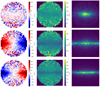 |
Fig. 1. Examples of line-of-sight velocity (left panels), dispersion (middle panels), and flux (right panels) maps for a galaxy with low rotation (upper panels), a clockwise rotating galaxy (middle panels), and an anticlockwise rotating galaxy (bottom panels). The maps are obtained from the kinematic data cubes generated by SIMSPIN by collapsing each data cube along the velocity axis, as described in Harborne et al. (2020). |
3.2. Dimensionality reduction algorithm
High-dimensional data may be difficult to handle and computationally expensive to process. Dimensionality reduction techniques allow the transformation of high-dimensional data into lower dimensional data minimising the loss of information, and facilitating in this way the visualisation and classification of the data sets.
UMAP is a dimensionality reduction algorithm first presented by McInnes et al. (2018). It serves as a manifold learning technique and, due to its good computational performance and scalability with dimensions and number of samples, it has a wide variety of applications in astronomy (e.g. Reis et al. 2021; Kim et al. 2021) and in other fields, such as bioinformatics and materials science. It is based on strong mathematical foundations that allow it to construct a representation in a low-dimensional space, which is topologically equivalent to the representation of the high-dimensional data (see McInnes et al. 2018, for details).
In this work we construct 30 px × 30 px kinematic images. Each map is reshaped to obtained 900-dimensional vectors. In Sect. 4, we study directly the line-of-sight velocity maps, and therefore the input of the algorithm are 900-dimensional data points. In Sect. 5, we include in the analysis the velocity dispersion and the flux information by concatenating to the line-of-sight velocity maps, velocity dispersion and flux maps, increasing the input dimension to 2700. Because of the differences in the magnitudes among the different data, we apply a uniform linear normalisation to each type of map by dividing each value by the maximum absolute value of the components across the whole data set. Therefore, the components of the velocity map are between −1 and 1, whereas for the dispersion and flux maps the values lie in the interval [0,1]. In both cases the high-dimensional data is projected into a bidimensional plane, thus obtaining an easy visualisation of the data and their subsequent clustering (see Appendix B for a discussion about the number of components of the output space).
In Table 1 we show the UMAP main (hyper)parameters we establish for each experiment in this work. In particular, n_neighbors defines the number of points in the local neighbourhood that the algorithm considers when it attempts to learn the manifold structure. Low values of n_neighbors implies that the algorithm focuses on very local structure, whereas setting large values yields a more global representation of the data. Another (hyper)parameter is the minimum distance (min_dist) at which the projected points are allowed to be. When this (hyper)parameter is low, the embeddings are clumpier with small connected components, while higher values should be used to preserve the broad structure. The reduced dimension space in which the data will be embedded is set with the (hyper)parameter n_components and the metrics used to compute distances in the input space defined by the metric (hyper)parameter.
UMAP and HDBSCAN (hyper)parameters set for each experiment.
3.3. Clustering algorithm
Clustering is the most commonly employed unsupervised ML algorithm. It aims to group objects that are in some sense similar (high intra-cluster similarity), while objects belonging to different groups are not similar (low inter-cluster similarity).
We chose the HDBSCAN (Campello et al. 2013) algorithm as our second step. This method outperforms other density-based clustering algorithms and is often used in astronomy (e.g. Katz et al. 2016; Kimm et al. 2018), and in a variety of disciplines like malware analysis, bioinformatics, and molecular dynamics. It is an ideal tool for unsupervised learning to define groups in data sets based on finding dense regions with the advantage that the number of clusters does not need to be specified. The set of significant clusters is obtained from the optimisation of the stability of the clusters given a minimum cluster size set before so that components with a number of elements below this threshold are considered spurious. The elements that cannot be assigned to any group are called outliers.
By using this algorithm, we find clear groups in the bidimensional projection depicting galaxies that share similar characteristics. We study the properties of each group to evaluate the usefulness of our method.
The HDBSCAN (hyper)parameters used in each experiment in this work are summarised in Table 1. The (hyper)parameter min_cluster_size defines the smallest number of elements in a group. To define how conservative the clustering might be, we can modify min_samples and alpha. Technically, min_samples is the number of samples in a neighbourhood for a point to be considered a core point. Large values of this (hyper)parameter result in a more conservative clustering where more points are considered noise in comparison with the clustering using low min_samples. Regarding alpha, it is a scale parameter related to the hierarchical algorithm, and it is also related to how conservative the clustering is. The default value of this parameter is 1 and higher values yield more conservative results. The minimum distance between clusters is given by cluster_selection_epsilon in the sense that clusters at distances below this threshold are merged. For more details about the algorithm see Campello et al. (2013).
We set all the (hyper)parameters in order to prioritise a clear visualisation of the trends among the clusters, and also to not be too restrictive, especially regarding the cluster sizes. Since UMSCANGALACTIK is an unsupervised method, we need human intervention in the analysis of the results that arise for different inputs, rather than relying on metrics like accuracy or sensitivity. The algorithms are sensitive to their (hyper)parameters, and the number of combination of (hyper)parameters is potentially huge. Hence, we can set their values for different inputs based on our astrophysical knowledge by keeping the ‘human-in-the-loop’. An important part of the challenges of this work is to find a combination of (hyper)parameters that allows us to find sensible and interesting results. Exploring heuristic methods to improve the (hyper)parameters selection is a research question itself and is beyond the scope of this paper.
4. Clustering of line-of-sight velocity maps
4.1. Clustering of edge-on galaxies
As a first approach, we use only the line-of-sight velocity maps of our galaxy sample as input of the algorithms described in Sect. 3 and study the variation of either physical or observational galaxy properties among the clusters obtained by UMSCANGALACTIK. In this subsection we observe galaxies edge-on, that is at an inclination of 90 degrees. Velocity maps are sensitive to the inclination at which a galaxy is observed because IFS can only measure line-of-sight velocity. Therefore, rotation is best noticed at high inclinations. In particular, at 90 degrees the line-of-sight is perpendicular to the total angular momentum.
In Fig. 2 we show a summary of the application of UMSCANGALACTIK to the line-of-sight velocity maps of edge-on galaxies. Hereafter, the colour bar limits are determined by the 10th and 90th percentiles of the property according to which the symbols are coloured. We quantify the distributions of the parameters involved in this analysis by approximating a probability density function (PDF) from the normalised histograms. The clustering method yields ∼3 per cent of outliers (grey dots). It is important to note that these outliers are located near the clustered points in the bidimensional embedding and that the variations of the physical and projected properties across the projection follow a continuous trend that includes the outliers.
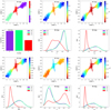 |
Fig. 2. Results of UMSCANGALACTIK applied to the line-of-sight velocity maps of our galaxy sample at inclination 90 degrees. Top row: HDBSCAN clusters in the UMAP bidimensional projection. The outliers of the method are shown as grey dots (left panel), and distributions of the projected parameters ε (middle panel) and λR (right panel) on the projection. Second row: Size of the clusters (left panel), and PDFs of ε (middle panel) and λR (right panel) for each cluster. Third row: Distribution of three-dimensional parameters D/T (left panel), T (middle panel), and λB (right panel) on the projection. Bottom row: PDFs of D/T (left panel), T (middle panel), and λB (right panel) for each cluster. The colour bar limits are fixed to the 10th and 90th percentile of the variables. |
We find three clusters, which we dubbed C0, C1, and C2. The central cluster, C2 (red), is populated by galaxies that are less disc-dominated with lower λB and that are more prolate (with higher values of T) than the galaxies in C0 (violet) and C1 (green). These properties are consistent with galaxies dominated by velocity dispersion, and in fact the D/T ratios of this population are low with most of the members having D/T < 0.2. Regarding the triaxiality parameter, a bimodal distribution can be seen with peaks at approximately T = 0.15 and T = 0.8. Galaxies in C2 with T ≤ 0.4 (around the first peak) also have higher disc fractions compared to the remaining galaxies with a median D/T of 0.21, being 0.16 and 0.26 the first and third quartiles, respectively. In contrast, the first, second (median), and third quartiles of D/T of C2 galaxies with T > 0.4 are 0.11, 0.13, and 0.16, respectively. It can also be seen from the figure that this low-rotation cluster has the lowest values of ε compared to the other two clusters, although a non-negligible number of galaxies in C2 have intermediate ellipticities overlapping with the distributions of ε of C0 and C1. The situation is similar to that of T: the highest ε galaxies in C2 have the highest D/T. For instance, the median D/T for galaxies in C2 with ε < 0.5 is 0.13, while the median D/T for the remaining galaxies is 0.22. Low projected ellipticities mean that the projected axis are more similar, and thus the galaxies are rounder. Galaxies in C2 have the lowest λB, as well as the lowest λR. This is what we expect since there is a significant correlation between the two spin parameters, regardless of the inclination. This is discussed in Appendix A where we show that the correlations between the two spins are present down to 20 degrees of inclination. For lower angles the Spearman coefficients are below 0.5.
It is clear in Fig. 2 that C0 and C1 are populated by oblate discy galaxies with the highest values of ε and both spin parameters. The disc fractions measured from the simulation of galaxies in C0 and C1 are systematically higher than those from C2. On the other hand, no significant differences can be found between the D/T of C0 and C1, as could be verified by a Brunner-Munzel test (Brunner & Munzel 2000)5. By comparing the PDFs in Fig. 2 for C0 and C1, we find very similar distributions of the parameters. This can also be quantified by the Brunner-Munzel test. The difference we observe is that galaxies in C0 and in C1 rotate in opposite directions regarding the line of sight (see Sect. 3). In order to explore the effect of the rotation direction in our classification, we repeat the procedure, but this time flipping the kinematic images of anticlockwise rotating galaxies, following the sign convention mentioned in Sect. 3.1. Thus, all input galaxies have the same direction. We show this in Fig. 3. As can be seen, UMSCANGALACTIK yields two clusters, being C1 (violet) associated with the highest disc fractions. C0 and C1 from Fig. 2 are unified by UMSCANGALACTIK in a single cluster. We conclude that the method is able to distinguish orientation without loss of information relevant to galaxy morphology.
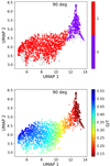 |
Fig. 3. Results of UMSCANGALACTIK applied to the line-of-sight velocity maps in which every galaxy has the same rotation direction. Top panel: HDBSCAN clusters in the UMAP bidimensional projection. The outliers of the method are shown as grey dots. Bottom panel: Distribution of D/T on the projection. |
Taking into account that we use kinematic information as the input for our method, it is interesting to assess the applicability of this method to the classification of SRs and FRs. This separation is widely studied in the literature (e.g. Emsellem et al. 2007, 2011; Veale et al. 2017; Brough et al. 2017; Greene et al. 2018; Lagos et al. 2018; Rosito et al. 2019a). Parametric classifications considering λR were proposed first by Emsellem et al. (2007, 2011) and in subsequent works (e.g. Cappellari 2016; Graham et al. 2018; van de Sande et al. 2021). Hereafter, we consider the parametric classification for SRs of van de Sande et al. (2021) shown in Eq. (1)
 (1)
(1)
where both parameters are measured within the half-light radius, also following Lagos et al. (2022).
In Fig. 4 (left panel) we show the λR-ε plane for all clustered galaxies following the colour-coding of Fig. 2. It is clear that the SR region according to van de Sande et al. (2021) is dominated by galaxies from C2, as expected. In fact, 71 per cent of the SRs belong to C2, whereas 17 per cent and 12 per cent belong to C0 and C1, respectively. Our approach may outperform the parametric classification since a non-negligible number of galaxies with low D/T belonging to C2 (23 per cent) would be classified as FRs with the parametric definition of van de Sande et al. (2021). In the middle panel of Fig. 4 it can be seen that these galaxies are those with the highest D/T within C2. Similarly, galaxies in the SR region belonging to C0 or C1 have the lowest D/T among these clusters (right panel). We note that physical parameters such as D/T do not depend on the inclination, and thus describe the fundamental properties of the galaxies.
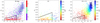 |
Fig. 4. Analysis of the λR − ε plane. Left panel: λR − ε plane for the clustered galaxies. The symbols depicting clusters follow the colour-coding in Fig. 2. Middle panel: λR − ε plane for galaxies of C2 colour-coded by D/T. Right panel: λR − ε plane for galaxies of C0 and C1 colour-coded by D/T. The colour bar limits are fixed to the 10th and 90th percentiles of the variables. We include in all cases the criterion in Eq. (1) depicted by the black solid lines. |
Automatic ML methods for galaxy classification yielding groups that distinguish galaxy rotation have been previously employed. From an input consisting of stellar population and kinematic maps for galaxies from MaNGA survey (Bundy et al. 2015), Sarmiento et al. (2021) obtain three galaxy clusters, one of which lies in the SR region of the λR-ε plane (their Fig. 3, first row), although the clusters significantly overlap. These galaxies are also notably older than those in the other two clusters, in agreement with galaxies from the EAGLE simulation (Rosito et al. 2019a).
We conclude that when we use only the information about line-of-sight velocity, we can obtain a clear separation between SRs and FRs. However, this requires that the rotation is clearly depicted in the kinematic maps, as we explain in the next subsection.
4.2. Effects of the inclination
In addition to studying the clustering of edge-on galaxies, we analyse the applicability of UMSCANGALACTIK to galaxies observed at different inclinations. The rotation is poorly seen at low inclinations, hence we assess how the method is affected by decreasing the angle of observation. In Table 2 we summarise the properties of the clustering at inclinations down to 20 degrees.
Summary of the HDBSCAN clustering at different inclinations using the line-of-sight velocity maps.
In Fig. 5 we show the application of UMSCANGALACTIK to galaxies at inclinations of 60, 45, 30, and 20 degrees and the distributions of D/T on the bidimensional projections (top and middle panels, respectively). In the first three cases we find three clusters, of which the central one, C2 (red), seems to have a notably smaller disc fraction. For the projection at 30 degrees the division of C1 (green) and C2 (red) is less clear, even though the clustering can identify the region with the lowest rotation. UMSCANGALACTIK cannot distinguish galaxies with the lowest D/T in a particular group when galaxies are observed at angles below 20 degrees.
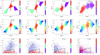 |
Fig. 5. Results of UMSCANGALACTIK applied to the line-of-sight velocity maps of our galaxy sample at different inclinations. Top panels: HDBSCAN clusters in the UMAP bidimensional projection of the line-of-sight velocity maps of galaxies observed at 60, 45, 30, and 20 degrees. The outliers of the method are shown as grey dots. Middle panels: Distributions of D/T on each projection. The colour bar limits are fixed to the 10th and 90th percentiles of the variables. Bottom panels: λR − ε plane. The symbols depict clusters following the same colour-coding as in the top panels. We include the criterion in Eq. (1) depicted by the black solid lines. |
In Fig. 5 (bottom panels), we also show the λR–ε plane. It is clear that the SRs region is dominated by galaxies from C2 in the first three cases, as expected. For inclinations of 90, 60, and 45 degrees, C2 includes above 70 per cent of the total SRs (according to Eq. (1)), whereas at 30 degrees this fraction decreases to 58 per cent. At 20 degrees, most galaxies are considered SRs according to the same criterion. The fraction of galaxies classified as SRs increases with decreasing inclination, as seen in Fig. 5 and Table 2. The rotation becomes less noticeable at lower inclinations, which can also be seen from their lower values of ε.
When applied to the sample considered in this work, UMSCANGALACTIK is robust enough to obtain a good classification of galaxies according to their level of rotation for inclinations greater than or equal to 45 degrees. To be conservative regarding the application of this method, we consider an inclination of 30 degrees a borderline case, although the quantities on the projection at 30 and 20 degrees still present clear trends for the sample studied in this paper. This is encouraging taking into account that our method relies on kinematic maps, which are sensitive to the inclination of the sources.
Regarding the outliers, we make the same observation as in Sect. 4.1. There is a continuous variation of the relevant properties across the bidimensional embeddings that involves both clustered and non-clustered galaxies. We can conclude this from the middle panels of Fig. 5 and the strong correlation between D/T and the other physical and projected properties. This pattern is also seen in the following sections. We note that galaxies close to each other in the projection have similar properties. UMSCANGALACTIK leverages this advantage of UMAP algorithm to obtain a more meaningful clustering.
5. Joint clustering of all kinematic map types
5.1. Clustering of edge-on galaxies
Our results indicate that clustering of only line-of-sight velocity maps is sufficient to describe the differences between SRs and FRs. In this section, we analyse the possibility of obtaining a meaningful clustering that captures more details about other features of galaxies, such as shape, by adding information from the velocity dispersion and flux maps. Hence, we apply UMSCANGALACTIK, as in the previous section, but first we concatenate the three types of kinematic maps (line-of-sight, dispersion, and flux maps) for galaxies observed at 90 degrees as input to perform the UMAP bidimensional projections.
In Fig. 6 we summarise the results of the application of UMSCANGALACTIK to the set of kinematic maps mentioned above. As can be seen in Fig. 6, the additional information brought in by the velocity dispersion and flux allow UMSCANGALACTIK to cluster galaxies in five different groups. Groups C3 (orange) and C4 (red) preferentially contain low-rotation galaxies, including 80 per cent of SRs defined by Eq. (1). The distributions of the parameters depicted in Fig. 6 for these clusters with low-rotation galaxies show clear differences in comparison with the other clusters, having notably lower D/T, lower spin parameters, lower ε, and higher T.
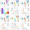 |
Fig. 6. Results of UMSCANGALACTIK applied to all kinematic map types of our galaxy sample at inclination 90 degrees. Top row: HDBSCAN clusters in the UMAP bidimensional projection. The outliers of the method are shown as grey dots (left panel), and distributions of the projected parameters ε (middle panel) and λR (right panel) on the projection. Second row: Size of the clusters (left panel), and PDFs of ε (middle panel) and λR (right panel) for each cluster. Third row: Distribution of three-dimensional parameters D/T (left panel), T (middle panel), and λB (right panel) on the projection. Bottom row: PDFs of D/T (left panel), T (middle panel), and λB (right panel) for each cluster. The colour bar limits are fixed to the 10th and 90th percentiles of the variables. |
By focusing on the comparison of the distributions of parameters from C3 and C4, in Fig. 6 it can be clearly seen that the triaxiality parameter distributions in C3 and C4 differ. By applying the Brunner-Munzel test, we conclude that the values of T in C3 are significantly higher than in C4, which means that galaxies are more prolate in the former. Through the same statistical test it is possible to determine that D/T values in C4 are systematically higher, but the differences between the medians of each distribution is low (0.02). In contrast, no significant differences among these two groups are seen regarding λB. This situation is similar when analysing the projected parameters. There are no significant differences in the values of λR, which is what we expect due to the strong correlation of this parameter with λB. On the other hand, the values of ε in C3 are lower, and this is consistent with the fact that galaxies in C3 are less dominated by rotation, and are thus seen to be rounder. Therefore, for edge-on galaxies, including the information of dispersion and flux leads to a refinement of low-rotation groups based primarily on galaxy shape. The addition of extra kinematic information results in an unsupervised classification that takes into account shape and rotation, and leads to a more accurate and meaningful classification of SRs. This may be useful to assist qualitative predictions of galaxy features when applied to samples with missing information on some parameters. Many efforts about the recovery of 3D shapes have been made recently, in particular those based on IFS, due to the importance of intrinsic shapes in the study of galaxies (Weijmans et al. 2014; Foster et al. 2017; Li et al. 2018; Ene et al. 2018). Bassett & Foster (2019) mention some of the difficulties these techniques face, such as the use of statistical methods to obtain distributions of three-dimensional shapes, the generalisation of theoretical models to different data sets, or the need of more tests of IFS shape measurement methods applied to large samples. They suggest using ML methods. Our approach, albeit qualitative, may be a direct way to predict shape parameters using the estimation of the distributions of those parameters for galaxies in the same group, and further exploration of the variation in galaxy shapes among clusters may be a useful way to tackle this task.
The clusters C0 (violet), C1 (light blue), and C2 (green) also present differences. From inspection of Fig. 6, it is clear that these clusters are populated by galaxies dominated by rotation, especially C0 and C1, and can thus be associated with FRs. The differences between the distributions of parameters of C0 and C1 are not clear from the figure. By applying the Brunner-Munzel test, we find that the D/T values in C0 are lower than those in C1, and the opposite behaviour is seen for the T parameter. The second trend is significant6 but weak: a p-value of 0.03. No significant differences between the values of λB and λR are found for galaxies in C0 and C1, and galaxies in C0 tend to have lower ε than those in C1. The main difference between C0 and C1 is the rotation orientation, in analogy to the situation presented in Sect. 4 for high-rotation galaxies. On the other hand, the distributions of the parameters for C2 shown in Fig. 6 are consistent with galaxies with intermediate rotation between SRs and the FRs. However, the number of galaxies populating C2 is much smaller than those in C0 and C1.
In Fig. 7 we show the UMAP projections considered in this section (Fig. 6) colour-coded by the clusters obtained using only the line-of-sight velocity maps studied in Sect. 4. As can be seen, the galaxies in C1 and C2 in this section belong to C0 of the clustering obtained in Sect. 4.1, and thus have the same rotation orientation.
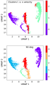 |
Fig. 7. Comparison between the clustering obtained using all kinematic map types and the line-of-sight velocity maps alone discussed in Sect. 4.1. Top panel: UMAP projection obtained from all kinematic maps according to the clustering obtained for the line-of-sight velocity maps, colour-coded as in Fig. 2. Bottom panel: Clustering in Fig. 6, repeated here for comparison. |
Figure 7 shows that the ‘extra’ clusters obtained with the information from all the kinematic map types are approximately subsets of the groups obtained using only the line-of-sight velocity maps. Therefore, these findings show that the refined clustering maintains the information provided by the line-of-sight velocity maps.
5.2. Effects of the inclination
In this subsection we study the robustness of UMSCANGALACTIK applying it to the kinematic maps with different inclinations. Based on the analysis performed in Sect. 4.2, we compare the result of the method when applied to the set of all kinematic map types at inclinations 90, 60, 45, and 30 degrees. Table 3 summarises the main properties of each clustering.
Summary of the HDBSCAN clustering at different inclinations using the three types of kinematic maps.
In the top and middle panels of Fig. 8 we show the clusters formed in the bidimensional projections of the set of all kinematic maps by the application of UMSCANGALACTIK and the same projection colour-coded following the clustering analysed in Sect. 4.2, respectively. For inclinations of 60 and 45 degrees (bottom panels), there are well-defined groups that present low-rotation galaxies. Around 70 per cent of the SRs classified according to Eq. (1) are included in these clusters at inclinations of 60 and 45 degrees, which is the same fraction observed in Sect. 4.2. In both cases the distributions of D/T of the groups with low-rotation galaxies show differences with the other clusters: they have notably lower values. Differences can be seen at 30 degrees; at this inclination UMSCANGALACTIK, using the only line-of-sight velocity, can better identify low-rotation galaxies, but, as we mentioned above, this is considered a borderline case and is not reliable enough for us to make robust conclusions.
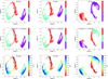 |
Fig. 8. Results of UMSCANGALACTIK applied to all kinematic map types of our galaxy sample at different inclinations. Top panels: HDBSCAN clusters in UMAP bidimensional projection of the set of all kinematic maps of galaxies observed at 60, 45, and 30 degrees. The outliers of the method are shown as grey dots. Middle panels: UMAP projection obtained from all kinematic map types according to the clustering obtained for the line-of-sight velocity maps discussed in Sect. 4, colour-coded as in Fig. 5Bottom panels: Distributions of D/T on each projection. The colour bar limits are fixed to the 10th and 90th percentiles of the variables. |
Again, at inclinations greater or equal to 45 degrees, the addition of other kinematic types maps maintains the information obtained by the clustering using solely velocity maps with the advantage that SRs may be more accurately described at high inclinations. Therefore, we suggest including all the information to achieve better classifications.
6. Analysis of slow and fast rotators
In this section we assess the possibility of achieving more meaningful clustering for galaxies with lower (or higher) levels of rotation by considering them separately. We select as input for our method the three types of kinematic maps of galaxies with λR, edge − on ≤ 0.2 and λR, edge − on > 0.2. Lagos et al. (2022) study a sample of the same simulation used in our work at z = 0 and note that most galaxies below a threshold of 0.2 in λR, edge − on have lower values of the spin parameter observed at any other inclination (van de Sande et al. 2021). This threshold is also considered to be a suitable separation in SRs and FRs in previous works (Lagos et al. 2018; Rosito et al. 2019a).
In the first case we find 609 galaxies in our sample with λR, edge − on ≤ 0.2. This constraint on the edge-on projected spin parameter includes 96 per cent SRs according to Eq. (1). We obtain three clusters and 35 outliers. In Fig. 9 we show an analysis of the clustering of the galaxies below this threshold. It can be seen that the separation in clusters in the UMAP projection is not as clear as those in the previous sections and that there is a continuous variation in the parameters among the three groups. Since rotation in all these galaxies is low, in Fig. 10 we look in detail at the 3D shapes in the different groups to analyse a meaningful clustering.
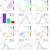 |
Fig. 9. Results of UMSCANGALACTIK applied to all the kinematic map types of galaxies with λR, edge − on ≤ 0.2 observed at 90 degrees. Top row: HDBSCAN clusters in the UMAP bidimensional projection. The outliers of the method are shown as grey dots (left panel), and distributions of the projected parameters ε (middle panel) and λR (right panel) on the projection. Second row: Size of the clusters (left panel), and PDFs of ε (middle panel) and λR (right panel) for each cluster. Third row: Distributions of three-dimensional parameters D/T (left panel), T (middle panel), and λB (right panel) on the projection. Bottom row: PDFs of D/T (left panel), T (middle panel), and λB (right panel) for each cluster. The colour bar limits are fixed to the 10th and 90th percentiles of the variables. |
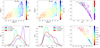 |
Fig. 10. Analysis of the 3D axis of galaxies with λR, edge − on ≤ 0.2. Top panels: Distributions of b/a (left panel) and b/a − c/a (middle panel) in the UMAP projection of the kinematic maps depicted in Fig. 9, and T vs b/a according to the clusters following the colour-coding in Fig. 9 (right panel). Bottom panels: PDFs of b/a (left panel) and b/a − c/a (middle panel), and T vs b/a for C0 colour-coded according to D/T (right panel). The colour bar limits are fixed to the 10th and 90th percentiles of the variables. |
A more discy group, C0 (violet), can be seen in Fig. 9, which also has notably lower values of T and higher λB, b/a, and b/a − c/a (Fig. 10) with respect to the other two groups. This is consistent with the right panels of Fig. 10 in the sense that in the plane T-b/a the region with low triaxiality parameters and high b/a ratios is dominated by galaxies from C0. From that figure it can also be seen that galaxies from C0 with the highest T and the lowest b/a are those with the lowest D/T within that cluster and hence we can associate this region with low amount of rotation. Moreover, there are differences between the projected parameters in C0 and C1 (green), as can be seen in the PDFs in Fig. 9, being these parameters lower in C1. However, the comparisons between the distributions of λR and ε from C0 and those of C2 (red) are unclear. It can be seen by means of the Brunner-Munzel test that ε from C0 have a weak trend (p-value ∼0.03) of being lower than those of C2 and that there is no systematic trend regarding λR. On the other hand, although C1 and C2 are both associated with galaxies in which the rotational component is almost negligible, the distributions of the parameters present systematic differences, as seen in the PDFs in Figs. 9 and 10 and quantified through the Brunner-Munzel test. Group C1 has the lowest D/T, ε, λR, b/a, b/a − c/a, and the highest T. The spin parameter λB can be considered lower in C1 than in C2, but this trend is weak (p-value 0.02).
Lagos et al. (2022) mention the importance of the visual classification of the kinematic maps to mitigate the inaccuracies of the parametric criteria based on the λR − ε plane (van de Sande et al. 2021). Lagos et al. (2022) visually classify their galaxies in the following groups: flat slow rotators (FSRs), round slow rotators (RSRs), prolate galaxies, 2σ galaxies, rotators, and unclear. We show that we can automatically perform a classification similar to the visual classification in Lagos et al. (2022).
The low triaxiality parameter for galaxies in C0 indicates that they are oblate and the fact that the major and middle axes have similar values but their difference with the minor axis is high is evidence that these galaxies are flatter. The values of T are high and b/a − c/a are low for C1 and C2, but the b/a ratios are significantly lower in C1, which means that C2 has rounder galaxies (axes of similar length), while galaxies in C1 are more prolate. Hence, we can associate C0, C1, and C2 respectively with the FSR, prolate, and RSR groups in Lagos et al. (2022). However, the fraction of galaxies in each group (see percentages in Fig. 9) is different to those reported by Lagos et al. (2022), who find a majority of FSR galaxies (48 per cent) followed by RSR (38 per cent) and prolate (10 per cent) galaxies.
The second group of galaxies, λR, edge − on > 0.2, consists of 1409 galaxies, and UMSCANGALACTIK yields a clustering depicting very clear groups with no outliers. In Fig. 11 we show the analysis of the two clusters obtained by our method. Very similar distributions of the parameters can be seen in the figure. Due to the high p-values of the two-sided Brunner-Munzel tests (above 0.5) in all cases, we conclude that there are no significant trends that the parameters in one cluster are greater than those in the other. Furthermore, the sizes of the two groups are similar. Galaxies in C0 and C1 rotate in opposite directions, and this is what UMSCANGALACTIK can capture.
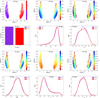 |
Fig. 11. Results of UMSCANGALACTIK applied to all the kinematic map types of galaxies with λR, edge − on > 0.2 observed at 90 degrees. Top row: HDBSCAN clusters in the UMAP bidimensional projection (left panel), and distributions of the projected parameters ε (middle panel) and λR (right panel) on the projection. Second row: Size of the clusters (left panel), and PDFs of ε (middle panel) and λR (right panel) for each cluster. Third row: Distributions of three-dimensional parameters D/T (left panel), T (middle panel), and λB (right panel) on the projection. Bottom row: PDFs of D/T (left panel), T (middle panel), and λB (right panel) for each cluster. The colour bar limits are fixed to the 10th and 90th percentiles of the variables. |
When using SRs alone as input the method yields similar conclusions to those presented in Sect. 5: galaxies with little rotation can be separated according to their shapes. Although we identified three groups instead of the two in Sect. 5.1 (C3 and C4), our clustering is weaker when the input does not have a rich enough variety of morphologies and kinematics. If only FRs are clustered, our method still identifies two clear groups differentiated by the orientation of galaxy rotation, as happens when the whole sample is considered (Sects. 4.1 and 5.1).
7. Mixing galaxies observed at different inclinations
Throughout this work we have clustered galaxies at a fixed inclination. Clustering kinematic maps from galaxies observed from different angles is more realistic than the procedures described in Sects. 4 and 5.
In this section we assess the applicability and the robustness of UMSCANGALACTIK when mixing galaxies at different inclinations. We use all kinematic map types, as in Sect. 5. The input of the method is the set of kinematic maps constructed for each galaxy from different inclinations. Due to the above-mentioned reasons related to the reliability of the method as a function of inclination, we consider angles of 90, 60, and 45 degrees. Hence, each galaxy is considered three times.
7.1. Clustering of galaxies from different inclinations
We obtain a supersample that includes three different inclinations (90, 60, and 45 degrees) for each galaxy, thus and consists of 2064 × 3 = 6192 elements. Therefore, we need to project 6192 high-dimensional points depicting the kinematic maps of each galaxy. After the application of the method, we obtain six clusters with 229 outliers, among which there are 153 distinct galaxies. The number of galaxies appearing at least once in the set of clusters is 2042.
In Fig. 12 we show the clustering obtained with the input studied in this section and a summary of the properties of its galaxies. We include physical and observational properties; the latter are sensitive to the angle of observation. The figure shows a division of galaxies with low levels of rotation (C4 and C5) and faster rotators (C0, C1, C2, and C3), as occurs when the inclination is fixed.
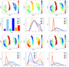 |
Fig. 12. Results of UMSCANGALACTIK applied to all the kinematic map types of our galaxy sample mixing three different inclinations. Top row: HDBSCAN clusters in the UMAP bidimensional projection. The outliers of the method are shown as grey dots (left panel), and distributions of the projected parameters ε (middle panel) and λR (right panel) on the projection. Second row: Size of the clusters (left panel), and PDFs of ε (middle panel) and λR (right panel) for each cluster. Third row: Distributions of three-dimensional parameters D/T (left panel), T (middle panel), and λB (right panel) on the projection. Bottom row: PDFs of D/T (left panel), T (middle panel), and λB (right panel) for each cluster. The colour bar limits are fixed to the 10th and 90th percentiles of the variables. |
Low-rotation clusters present differences in the distributions of the parameters. By means of the Brunner-Munzel test, we find that galaxies in C4 have significantly lower D/T, lower λB, lower λR, lower ε, and higher T than those from C5, which is consistent with having a smaller disc component.
The differences between the parameter distribution from C1 and C3 are less noticeable in Fig. 12. Statistically, the Brunner-Munzel test shows that disc fractions in C1 are greater than those in C3, but the trend is weak since the p-value is 0.01. As in Sect. 5, the smallest clusters, C0 and C2, present parameters with intermediate values between SRs and FRs. The groups C0+C1 and C2+C3 are populated by galaxies rotating in opposite directions.
We show that when considering galaxies observed at different high inclinations, UMSCANGALACTIK is still useful and the clustering meaningful. These considerations yield similar conclusions to those of the edge-on galaxies study.
7.2. The robustness of our method
In this subsection we check that, in most cases, the different instances of the same galaxy (i.e. the kinematic maps for each galaxy observed at 90, 60, and 45 degrees) are clustered in the same group after the application of UMSCANGALACTIK. We detail in Table 4 the number of elements within each group with the number of repetitions for each distinct galaxy.
Number of galaxies and repetitions in each group obtained when applying UMSCANGALACTIK to the mixture of the kinematic maps for the same galaxies observed at three different inclinations.
As stated in Table 4, in C1 and C3 the vast majority of the galaxies appear three times in the same cluster, that is, they receive the same classification regardless of the inclination. The situation is similar for the low-rotation clusters, C4 and C5; although the fraction of robustly classified galaxies is lower, it is still high. In C0 and C2, these fractions of galaxies repeated three times are the lowest, which means that galaxies in these groups are more susceptible to inclination effects.
The result mentioned above yields a lower bound for robustly classified galaxies. We can affirm that 1640 out of 2064 galaxies (80 per cent) are robustly classified by UMSCANGALACTIK. This fraction may be higher if we take into account that not all 2064 galaxies have been clustered and that we do not consider galaxies repeated twice in a particular cluster. This value is conservative, but it is good enough to conclude that UMSCANGALACTIK is robust even if the inclinations in the range between 45 deg and 90 deg are mixed.
The sizes of C0 and C2 are notably smaller than those of the other clusters, as can be seen from Table 4 and from the bar plot in Fig. 12. In both clusters, the number of elements depicts five per cent of the total input size. These clusters would be joined to C1 and C3, respectively, if we applied a more restrictive condition regarding the minimum cluster size. Moreover, galaxies in these FR clusters share similar properties in terms of shape and kinematic parameters, as mentioned above. If this were the case, we would obtain two larger clusters of sizes 2198 (C0 + C1) and 2350 (C2 + C3), of which 94 per cent and 89 per cent of their galaxies are correctly classified regardless of their inclination. In addition, taking into account that rotation is less noticeable as the inclination decreases and that our method is then not able to separate SRs according to shape in different groups (as seen in Sect. 5.2), joining C4 and C5 in a single cluster (C4 + C5) would also be reasonable when analysing the robustness of UMSCANGALACTIK. We would obtain 78 per cent of properly classified SRs galaxies in C4 + C5. Following this idea, by adding the number of robustly classified galaxies in C0 + C1, C2 + C3, and C4 + C5, the above-mentioned bound increases to 90 per cent.
8. Conclusions
In this work we have defined clear steps to perform an unsupervised kinematic morphology classification of a sample of galaxies from the EAGLE simulation (Schaye et al. 2015; Crain et al. 2015). Since the input of UMSCANGALACTIK are kinematic maps that mimic IFS observations, it can be applied either to observational data sets or to other simulations. These maps are computed at different inclinations. We project the maps (considered as high-dimensional points) to a bidimensional space using the UMAP algorithm (McInnes et al. 2018) followed by the application of the HDBSCAN clustering (Campello et al. 2013). We identify the advantages and limitations of this methodology and conclude that it may be useful for defining unsupervised classifications of galaxies that capture their main morphological properties based on physical parameters.
The main results of this study are the following:
-
Line-of-sight velocity maps as input are sufficient to perform a good classification in SRs and FRs for edge-on galaxies. Most galaxies in the cluster with the lowest values of D/T are classified as SRs according to Eq. (1) (van de Sande et al. 2021), as shown in Fig. 4. However, there is a fraction of these galaxies that would be considered FRs using this parametric criterion despite the low disc fractions. Therefore, UMSCANGALACTIK may be considered more accurate than those based on the observational projected parameters (λR and ε) since it provides a clearer separation regarding the rotational component. Furthermore, galaxies in clusters associated with high rotation are separated by the direction of rotation. We show that this is an advantage of UMSCANGALACTIK in the sense that it allows the extraction of this information without introducing a false dimension that may lead to underperformance of the classification. Although not relevant to explain the kinematic morphologies of galaxies, this information could be useful to study the relative rotation between galaxies.
-
By adding the velocity dispersion and flux maps to the analysis, edge-on galaxies with low rotation are divided in two groups (C3 and C4) which differ mainly in the triaxiality parameter yielding a refinement of the low-rotation cluster found in Sect. 4 (Fig. 6). Using hypothesis testing, we also find systematic differences in the values of D/T and ε from C3 and C4, and no significant difference regarding the spin parameters. Among the clusters with galaxies with higher levels of rotation (C0, C1, and C2), C0 and C1 differ mainly in the rotation orientation. The distributions of the parameters for galaxies in C2 present markedly noticeable differences with respect to the others, but its size is too small to draw a robust conclusion.
-
Figures 7 and 8 show that at inclinations greater than or equal to 45 degrees, the clusters obtained in Sect. 5 can be considered subsets of the groups obtained in the analysis performed in Sect. 4. Therefore, the addition of the dispersion and flux maps preserves the information provided by the velocity maps. Since the use of all kinematic map types yields a more detailed description of low-rotation edge-on galaxies, we suggest including them when performing morphological classification using UMSCANGALACTIK.
-
Because the input data considered for our analysis consist of IFS kinematic maps, which are sensitive to the angle of observation, UMSCANGALACTIK is useful when galaxies are observed at inclinations at which rotation can be clearly distinguished. When the inclination is 30 degrees, the fraction of SRs (according to the parameter definition) identified in the low-rotation cluster decreases significantly with respect to higher inclinations, and the division in clusters is less clear. We adopt a conservative criterion, preferring angles greater than or equal to 45 degrees.
-
When applying UMSCANGALACTIK exclusively to slow rotating galaxies, we can identify groups with different shapes. However, the separation between groups in the UMAP projection is not as clear as when galaxies with a variety of morphologies and kinematics are clustered together. On the other hand, the method divides a sample of FRs according to the rotation orientation, and the parameter distributions present no significant differences among the two groups.
-
When the input consists of galaxies observed at different inclinations, UMSCANGALACTIK still clearly differentiates SRs and FRs. The former are divided into two groups, as happens when only edge-on galaxies are considered (Sect. 5.1). Galaxies with high levels of rotation are separated according to the direction of rotation. Furthermore, we find clusters with intermediate parameters between SRs and FRs, even though these clusters are very small in comparison to the others. An input that mixes galaxies observed at different inclinations is more realistic, and the fact that our method still obtains a meaningful clustering is encouraging. Furthermore, UMSCANGALACTIK is robust with respect to the inclinations of the input galaxies. It can be seen that in at least ∼80 per cent of the cases, the different instances of each galaxy are classified in the same group. If we apply a more restrictive clustering algorithm, this fraction can increase to ∼90 per cent. When allowing finer clustering, our method produces some mixing within groups, but it is still able to clearly separate SRs and FRs.
The methodology presented in this paper has proven to be accurate for a sample of mock galaxies and has succeeded in identifying their intrinsic properties and their projected parameters. The need to observe galaxies at high inclinations can be mitigated by predicting how the kinematic maps of galaxies observed in an arbitrary inclination would be seen edge-on. Dynamical models (Cappellari 2008) have been used for similar tasks in the last decade.
The next stage is to asses its applicability to observational data sets and to a new generation of simulations. Testing UMSCANGALACTIK on mock inputs that are more similar to observations would be an enriching and necessary step before applying it to real observations. We can obtain more diverse input samples by choosing different distances and inclination angles to build the SIMSPIN data cubes in addition to changing the user-specified point spread function (Harborne et al. 2020). There are other considerations to keep in mind when dealing with IFS, such as the need for a minimum signal-to-noise ratio to measure the line-of-sight velocity. Voronoi tessellation binning (Cappellari & Copin 2003) can be used for unbiased recovery of this kinematic information, and it may be interesting to explore methods like the procedure proposed by Walo-Martín et al. (2020).
Machine learning algorithms are becoming mandatory to study astronomy. The use of unsupervised techniques has the potential to increase our ability to scrutinise large data sets and to extract information with physical meaning.
We use the EAGLE public database (McAlpine et al. 2016).
The Brunner-Munzel test is a statistical test used to assess the stochastic equality of two samples without assuming that the shapes of the underlying distributions are the same.
We consider a level of significance of 0.05, which is commonly used in hypothesis testing.
Acknowledgments
PBT acknowledges partial funding by Fondecyt 1200703/2020 (ANID), ANID Basal Project FB210003, and Nucleo Milenio ANID ERIS. SP acknowledges support through PIP CONICET 11220170100638CO.
References
- Abraham, R. G., van den Bergh, S., & Nair, P. 2003, ApJ, 588, 218 [NASA ADS] [CrossRef] [Google Scholar]
- Artale, M. C., Pedrosa, S. E., Tissera, P. B., Cataldi, P., & Di Cintio, A. 2019, A&A, 622, A197 [NASA ADS] [CrossRef] [EDP Sciences] [Google Scholar]
- Bacon, R., Copin, Y., Monnet, G., et al. 2001, MNRAS, 326, 23 [Google Scholar]
- Bahé, Y. M., Barnes, D. J., Dalla Vecchia, C., et al. 2017, MNRAS, 470, 4186 [Google Scholar]
- Ball, N. M., & Brunner, R. J. 2010, Int. J. Mod. Phys. D, 19, 1049 [Google Scholar]
- Baron, D. 2019, ArXiv e-prints [arXiv:1904.07248] [Google Scholar]
- Bassett, R., & Foster, C. 2019, MNRAS, 487, 2354 [Google Scholar]
- Bignone, L. A., Pedrosa, S. E., Trayford, J. W., Tissera, P. B., & Pellizza, L. J. 2020, MNRAS, 491, 3624 [Google Scholar]
- Binney, J. 1978, MNRAS, 183, 501 [NASA ADS] [Google Scholar]
- Bois, M., Emsellem, E., Bournaud, F., et al. 2011, MNRAS, 416, 1654 [Google Scholar]
- Bongiovanni, Á., Ramón-Pérez, M., Pérez García, A. M., et al. 2019, A&A, 631, A9 [NASA ADS] [CrossRef] [EDP Sciences] [Google Scholar]
- Brough, S., van de Sande, J., Owers, M. S., et al. 2017, ApJ, 844, 59 [Google Scholar]
- Brunner, E., & Munzel, U. 2000, Biom. J., 42, 17 [CrossRef] [Google Scholar]
- Bruzual, G., & Charlot, S. 2003, MNRAS, 344, 1000 [NASA ADS] [CrossRef] [Google Scholar]
- Bryant, J. J., Owers, M. S., Robotham, A. S. G., et al. 2015, MNRAS, 447, 2857 [Google Scholar]
- Bullock, J. S., Dekel, A., Kolatt, T. S., et al. 2001, ApJ, 555, 240 [NASA ADS] [CrossRef] [Google Scholar]
- Bundy, K., Bershady, M. A., Law, D. R., et al. 2015, ApJ, 798, 7 [Google Scholar]
- Campello, R. J. G. B., Moulavi, D., & Sander, J. 2013, in Advances in Knowledge Discovery and Data Mining, eds. J. Pei, V. S. Tseng, L. Cao, H. Motoda, & G. Xu (Berlin, Heidelberg: Springer, Berlin Heidelberg), 160 [Google Scholar]
- Cappellari, M. 2008, MNRAS, 390, 71 [NASA ADS] [CrossRef] [Google Scholar]
- Cappellari, M. 2016, ARA&A, 54, 597 [Google Scholar]
- Cappellari, M., & Copin, Y. 2003, MNRAS, 342, 345 [Google Scholar]
- Cataldi, P., Pedrosa, S. E., Tissera, P. B., & Artale, M. C. 2021, MNRAS, 501, 5679 [NASA ADS] [CrossRef] [Google Scholar]
- Chabrier, G. 2003, PASP, 115, 763 [Google Scholar]
- Chadha, K. S. 2007, Astron. Now, 21, 28 [Google Scholar]
- Cheng, T.-Y., Huertas-Company, M., Conselice, C. J., et al. 2021, MNRAS, 503, 4446 [NASA ADS] [CrossRef] [Google Scholar]
- Chisari, N., Codis, S., Laigle, C., et al. 2015, MNRAS, 454, 2736 [NASA ADS] [CrossRef] [Google Scholar]
- Combes, F. 2009, ASP Conf. Ser., 419, 31 [NASA ADS] [Google Scholar]
- Conselice, C. J. 2003, ApJS, 147, 1 [NASA ADS] [CrossRef] [Google Scholar]
- Conselice, C. J. 2014, ARA&A, 52, 291 [CrossRef] [Google Scholar]
- Correa, C. A., Schaye, J., Clauwens, B., et al. 2017, MNRAS, 472, L45 [Google Scholar]
- Crain, R. A., Schaye, J., Bower, R. G., et al. 2015, MNRAS, 450, 1937 [NASA ADS] [CrossRef] [Google Scholar]
- Dalla Vecchia, C., & Schaye, J. 2012, MNRAS, 426, 140 [NASA ADS] [CrossRef] [Google Scholar]
- Davies, R. L., Efstathiou, G., Fall, S. M., Illingworth, G., & Schechter, P. L. 1983, ApJ, 266, 41 [NASA ADS] [CrossRef] [Google Scholar]
- de Diego, J. A., Nadolny, J., Bongiovanni, Á., et al. 2020, A&A, 638, A134 [NASA ADS] [CrossRef] [EDP Sciences] [Google Scholar]
- de Vaucouleurs, G. 1948, Ann. dAstrophys., 11, 247 [NASA ADS] [Google Scholar]
- Deng, X.-F. 2013, Res. Astron. Astrophys., 13, 651 [Google Scholar]
- Djorgovski, S., & Davis, M. 1987, ApJ, 313, 59 [Google Scholar]
- Dolag, K., Borgani, S., Murante, G., & Springel, V. 2009, MNRAS, 399, 497 [Google Scholar]
- Dubois, Y., Peirani, S., Pichon, C., et al. 2016, MNRAS, 463, 3948 [Google Scholar]
- Emsellem, E., Cappellari, M., Krajnović, D., et al. 2007, MNRAS, 379, 401 [Google Scholar]
- Emsellem, E., Cappellari, M., Krajnović, D., et al. 2011, MNRAS, 414, 888 [Google Scholar]
- Ene, I., Ma, C.-P., Veale, M., et al. 2018, MNRAS, 479, 2810 [Google Scholar]
- Fisher, D. B., & Drory, N. 2008, AJ, 136, 773 [NASA ADS] [CrossRef] [Google Scholar]
- Foster, C., van de Sande, J., D’Eugenio, F., et al. 2017, MNRAS, 472, 966 [NASA ADS] [CrossRef] [Google Scholar]
- Graham, M. T., Cappellari, M., Li, H., et al. 2018, MNRAS, 477, 4711 [Google Scholar]
- Greene, J. E., Leauthaud, A., Emsellem, E., et al. 2018, ApJ, 852, 36 [NASA ADS] [CrossRef] [Google Scholar]
- Haardt, F., & Madau, P. 2001, in Clusters of Galaxies and the High Redshift Universe Observed in X-rays, ed. D. M. Neumann, & J. T. T. Van, 64 [Google Scholar]
- Harborne, K. E., Power, C., Robotham, A. S. G., Cortese, L., & Taranu, D. S. 2019, MNRAS, 483, 249 [NASA ADS] [CrossRef] [Google Scholar]
- Harborne, K. E., Power, C., & Robotham, A. S. G. 2020, PASA, 37 [CrossRef] [Google Scholar]
- Hocking, A., Geach, J. E., Sun, Y., & Davey, N. 2018, MNRAS, 473, 1108 [CrossRef] [Google Scholar]
- Howard, E. M. 2017, ASP Conf. Ser., 512, 245 [NASA ADS] [Google Scholar]
- Hubble, E. P. 1926, ApJ, 64, 321 [Google Scholar]
- Illingworth, G. 1977, ApJ, 218, L43 [Google Scholar]
- Ivezić, Ž., Kahn, S. M., Tyson, J. A., et al. 2019, ApJ, 873, 111 [Google Scholar]
- Jesseit, R., Cappellari, M., Naab, T., Emsellem, E., & Burkert, A. 2009, MNRAS, 397, 1202 [NASA ADS] [CrossRef] [Google Scholar]
- Katz, H., Lelli, F., McGaugh, S. S., et al. 2016, MNRAS, 466, 1648 [Google Scholar]
- Khalifa, N. E. M., Taha, M. H. N., Hassanien, A. E., & Selim, I. M. 2017, ArXiv e-prints [arXiv:1709.02245] [Google Scholar]
- Kim, Y., Telea, A. C., Trager, S. C., & Roerdink, J. B. T. M. 2021, ArXiv e-prints [arXiv:2110.00317] [Google Scholar]
- Kimm, T., Haehnelt, M., Blaizot, J., et al. 2018, MNRAS, 475, 4617 [CrossRef] [Google Scholar]
- Kormendy, J., & Bender, R. 2012, ApJS, 198, 2 [Google Scholar]
- Kremer, J., Stensbo-Smidt, K., Gieseke, F., Steenstrup Pedersen, K., & Igel, C. 2017, IEEE Intelligent Systems, 32, 16 [CrossRef] [Google Scholar]
- Lagos, C. D. P., Schaye, J., Bahé, Y., et al. 2018, MNRAS, 476, 4327 [Google Scholar]
- Lagos, C. D. P., Emsellem, E., van de Sande, J., et al. 2022, MNRAS, 509, 4372 [Google Scholar]
- Lahav, O., Naim, A., Buta, R. J., et al. 1995, Science, 267, 859 [CrossRef] [Google Scholar]
- Laureijs, R., Amiaux, J., Arduini, S., et al. 2011, ArXiv e-prints [arXiv:1110.3193] [Google Scholar]
- Li, H., Mao, S., Cappellari, M., et al. 2018, MNRAS, 476, 1765 [NASA ADS] [Google Scholar]
- Lotz, J. M., Primack, J., & Madau, P. 2004, AJ, 128, 163 [NASA ADS] [CrossRef] [Google Scholar]
- LSST Science Collaboration (Abell, P. A., et al.) 2009, ArXiv e-prints [arXiv:0912.0201] [Google Scholar]
- Marin, M., Sucar, L., Gonzalez, J., & Diaz, R. 2013, A Hierarchical Model for Morphological Galaxy Classification, 438 [Google Scholar]
- McAlpine, S., Helly, J. C., Schaller, M., et al. 2016, Astron. Comput., 15, 72 [NASA ADS] [CrossRef] [Google Scholar]
- McInnes, L., Healy, J., & Melville, J. 2018, ArXiv e-prints [arXiv:1802.03426] [Google Scholar]
- Mittal, A., Soorya, A., Nagrath, P., & Hemanth, D. J. 2019, Earth Sci. Inform., 13, 601 [Google Scholar]
- Naab, T., Oser, L., Emsellem, E., et al. 2014, MNRAS, 444, 3357 [Google Scholar]
- Papovich, C., Giavalisco, M., Dickinson, M., Conselice, C. J., & Ferguson, H. C. 2003, ApJ, 598, 827 [NASA ADS] [CrossRef] [Google Scholar]
- Pedrosa, S. E., & Tissera, P. B. 2015, A&A, 584, A43 [NASA ADS] [CrossRef] [EDP Sciences] [Google Scholar]
- Peebles, P. J. E. 1969, ApJ, 155, 393 [Google Scholar]
- Penoyre, Z., Moster, B. P., Sijacki, D., & Genel, S. 2017, MNRAS, 468, 3883 [Google Scholar]
- Planck Collaboration I. 2014, A&A, 571, A1 [NASA ADS] [CrossRef] [EDP Sciences] [Google Scholar]
- Planck Collaboration XVI. 2014, A&A, 571, A16 [Google Scholar]
- Portillo, S. K. N., Parejko, J. K., Vergara, J. R., & Connolly, A. J. 2020, AJ, 160, 45 [Google Scholar]
- Raddick, J., Lintott, C. J., Schawinski, K., et al. 2007, BAAS, 39, 892 [NASA ADS] [Google Scholar]
- Reis, I., Rotman, M., Poznanski, D., Prochaska, J. X., & Wolf, L. 2021, Astron. Comput., 34, 100437 [NASA ADS] [CrossRef] [Google Scholar]
- Rosas-Guevara, Y. M., Bower, R. G., Schaye, J., et al. 2015, MNRAS, 454, 1038 [NASA ADS] [CrossRef] [Google Scholar]
- Rosito, M. S., Pedrosa, S. E., Tissera, P. B., et al. 2018, A&A, 614, A85 [NASA ADS] [CrossRef] [EDP Sciences] [Google Scholar]
- Rosito, M. S., Tissera, P. B., Pedrosa, S. E., & Lagos, C. D. P. 2019a, A&A, 629, L3 [NASA ADS] [CrossRef] [EDP Sciences] [Google Scholar]
- Rosito, M. S., Tissera, P. B., Pedrosa, S. E., & Rosas-Guevara, Y. 2019b, A&A, 629, A37 [NASA ADS] [CrossRef] [EDP Sciences] [Google Scholar]
- Rosito, M. S., Pedrosa, S. E., Tissera, P. B., et al. 2021, A&A, 652, A44 [NASA ADS] [CrossRef] [EDP Sciences] [Google Scholar]
- Sánchez, S. F., Kennicutt, R. C., Gil de Paz, A., et al. 2012, A&A, 538, A8 [Google Scholar]
- Sánchez Almeida, J., & Allende Prieto, C. 2013, ApJ, 763, 50 [CrossRef] [Google Scholar]
- Sánchez Almeida, J., Aguerri, J. A. L., Muñoz-Tuñón, C., & de Vicente, A. 2010, ApJ, 714, 487 [Google Scholar]
- Sarmiento, R., Huertas-Company, M., Knapen, J. H., et al. 2021, ApJ, 921, 177 [NASA ADS] [CrossRef] [Google Scholar]
- Scannapieco, C., Tissera, P. B., White, S. D. M., & Springel, V. 2008, MNRAS, 389, 1137 [CrossRef] [Google Scholar]
- Schaye, J., & Dalla Vecchia, C. 2008, MNRAS, 383, 1210 [Google Scholar]
- Schaye, J., Crain, R. A., Bower, R. G., et al. 2015, MNRAS, 446, 521 [Google Scholar]
- Schulze, F., Remus, R.-S., Dolag, K., et al. 2018, MNRAS, 480, 4636 [Google Scholar]
- Scott, N., van de Sande, J., Croom, S. M., et al. 2018, MNRAS, 481, 2299 [Google Scholar]
- Selim, I., Arabi, E., & El, M. B., 2016, Int. J. Comput. Appl., 137, 4 [Google Scholar]
- Sérsic, J. L. 1968, Atlas de Galaxias Australes (Cordoba, Argentina: Observatorio Astronomico) [Google Scholar]
- Springel, V., Yoshida, N., & White, S. D. M. 2001, New Astron., 6, 79 [Google Scholar]
- Springel, V., Di Matteo, T., & Hernquist, L. 2005, MNRAS, 361, 776 [Google Scholar]
- Storrie-Lombardi, M. C., Lahav, O., Sodre, L. J., & Storrie-Lombardi, L. 1992, BAAS, 181, 65.08 [NASA ADS] [Google Scholar]
- Tissera, P. B. 2000, ApJ, 534, 636 [NASA ADS] [CrossRef] [Google Scholar]
- Tissera, P. B., & Dominguez-Tenreiro, R. 1998, MNRAS, 297, 177 [NASA ADS] [CrossRef] [Google Scholar]
- Tissera, P. B., White, S. D. M., & Scannapieco, C. 2012, MNRAS, 420, 255 [NASA ADS] [CrossRef] [Google Scholar]
- Tissera, P. B., Machado, R. E. G., Sanchez-Blazquez, P., et al. 2016a, A&A, 592, A93 [NASA ADS] [CrossRef] [EDP Sciences] [Google Scholar]
- Tissera, P. B., Pedrosa, S. E., Sillero, E., & Vilchez, J. M. 2016b, MNRAS, 456, 2982 [CrossRef] [Google Scholar]
- Tissera, P. B., Rosas-Guevara, Y., Bower, R. G., et al. 2019, MNRAS, 482, 2208 [Google Scholar]
- Tohill, C., Ferreira, L., Conselice, C. J., Bamford, S. P., & Ferrari, F. 2021, ApJ, 916, 4 [NASA ADS] [CrossRef] [Google Scholar]
- Tonini, C., Mutch, S. J., Croton, D. J., & Wyithe, J. S. B. 2016, MNRAS, 459, 4109 [NASA ADS] [CrossRef] [Google Scholar]
- Uzeirbegovic, E., Geach, J. E., & Kaviraj, S. 2020, MNRAS, 498, 4021 [CrossRef] [Google Scholar]
- van de Sande, J., Vaughan, S. P., Cortese, L., et al. 2021, MNRAS, 505, 3078 [NASA ADS] [CrossRef] [Google Scholar]
- van de Ven, G., & van der Wel, A. 2021, ApJ, 914, 45 [NASA ADS] [CrossRef] [Google Scholar]
- Veale, M., Ma, C.-P., Thomas, J., et al. 2017, MNRAS, 464, 356 [Google Scholar]
- Vika, M., Vulcani, B., Bamford, S. P., Häußler, B., & Rojas, A. L. 2015, A&A, 577, A97 [NASA ADS] [CrossRef] [EDP Sciences] [Google Scholar]
- Walo-Martín, D., Falcón-Barroso, J., Dalla Vecchia, C., Pérez, I., & Negri, A. 2020, MNRAS, 494, 5652 [CrossRef] [Google Scholar]
- Weijmans, A.-M., de Zeeuw, P. T., Emsellem, E., et al. 2014, MNRAS, 444, 3340 [Google Scholar]
- Wiersma, R. P. C., Schaye, J., & Smith, B. D. 2009, MNRAS, 393, 99 [NASA ADS] [CrossRef] [Google Scholar]
- Yoon, Y., & Im, M. 2020, ApJ, 893, 117 [NASA ADS] [CrossRef] [Google Scholar]
Appendix A: Correlation between λB and λR
In this work we analyse the distributions of two spin parameters, λB (Bullock et al. 2001) and λR (Emsellem et al. 2007), for galaxies observed at different inclinations. We note that the former is obtained from the particle 3D distributions, and therefore does not depend on the inclination. This parameter (λB) plays a role in the description of the variation of the specific angular momentum as a function of the halo mass. Bullock et al. (2001) propose it as an alternative definition of the spin parameter, generalising the definition previously used in the literature (e.g. Peebles 1969). On the other hand, the spin parameter defined by Emsellem et al. (2007), λR, although it also quantifies angular momentum, is computed from bidimensional kinematic information; observational descriptions of rotation and shape based on it are more accurate than those obtained from anisotropy diagrams (Illingworth 1977; Binney 1978; Davies et al. 1983). Harborne et al. (2019) find an approximate functional relation between these two parameters from a set of N-body realisation of galaxies.
We study the monotonic (increasing) relationship between these parameters by means of the Spearman correlation coefficient. In Table A.1 we show these coefficients computed at different inclinations. Although in all cases the low p-values (∼0) indicate a significant relationship, it can be appreciated that the coefficients decrease with the angle. This is related to the fact that the rotation becomes less noticeable at low inclinations.
Figure A.1 shows λB as a function of ε instead of the λR − ε plane widely used to separate SRs and FRs. We measure ε projected at different inclinations. It can be seen that at low inclinations galaxies are seen to be rounder than they would be at high inclinations, while λB remains the same. However, the correlation between the two spin parameters may justify the use of λB instead of λR to analyse the relation between rotation and shape. Because of the differences in the Spearman coefficients, the analysis would be more reliable at higher inclinations.
Spearman coefficients between λB and λR computed at different inclinations.
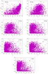 |
Fig. A.1. λB as a function of ε where ellipticities are computed at different inclinations. The decrease in the values of ε with decreasing inclination indicates that galaxies are seen to be rounder when observed at low inclinations. |
Appendix B: Dimensionality of the output space
In this Appendix we explore the intrinsic dimensionality of the problem and discuss how the method would be impacted if more than two dimensions are considered in the clustering algorithm.
B.1. Analysis of the number of dimensions
Throughout this work, we focus on the bidimensional projections on which we applied the HDBSCAN clustering algorithm. It is reasonable to be concerned about the loss of information when reducing very high-dimensional data to only two components. However, we show that UMSCANGALACTIK is able to produce galaxy groups that are meaningful without using labels. Furthermore, classical works on galaxy kinematics (e.g. Emsellem et al. 2007, 2011; Cappellari 2016; van de Sande et al. 2021) divide SRs and FRs using only two dimensions (ε and λR), and these classifications are proven to be insightful for subsequent studies.
Because UMAP lacks the interpretability of the dimensions of the embeddings, as well as a quantification of the explained variance (McInnes et al. 2018), we turn to PCA to obtain an approximation of the information retained by the dimensionality reduction process. PCA has been used to study galaxy morphology. For instance, Uzeirbegovic et al. (2020) applied PCA to galaxy images and found that 85 per cent of the variance could be explained using just two components.
In Table B.1 we show the percentage of variance that a PCA algorithm would explain for the line-of-sight velocity maps (Sect. 4) and the set of all the types of kinematic maps (Sect. 5). This linear algorithm leads to non-negligible information loss with the explained variance ranging from 47.6 per cent to 68.6 per cent. However, a non-linear method such as UMAP outperforms other algorithms in the preservation of global structure and may lead to better performance compared to PCA, for example when using classifiers such as k-nearest neighbours (McInnes et al. 2018).
Analysis of the explained variance (% var) for two and ten principal components (PCs) and number of PCs needed to explain 75 per cent of the variance for the PCA algorithm applied to the sample of (a) line-of-sight velocity maps (Experiment 1) and (b) three types of kinematic maps (Experiment 2) for different inclinations.
B.2. Clustering on a ten-dimensional UMAP embedding
To explore the effects of using a larger number of dimensions for the clustering part of this work, we conduct experiments using ten-dimensional embeddings. In Fig. B.1 we show the bidimensional projections computed in Sect. 4.1 coloured by the HDBSCAN clustering of the ten-dimensional UMAP embeddings. We use a small (hyper)parameter grid that includes the parameters utilised for our analysis (Table 1, Experiment 1). We modify n_neighbors, min_dist, and set n_components = 10. In all cases we find a large number of outliers, especially those in which we observe more than three clusters. In general we find that using ten components instead of two does not improve the quality of the clustering significantly or make it more meaningful or robust. As mentioned in Sect. 3, the selection of (hyper)parameters is not straightforward and a larger number of dimensions appears to make the clustering more sensitive to small changes of (hyper)parameter values.
Although it would be worthwhile to explore the potential improvements we would obtain by clustering higher-dimensional embeddings, the method we present here leads to meaningful classifications by using bidimensional projections. This exploration will be analysed in a future work, and may be helpful in data leveraging and generalisation of UMSCANGALACTIK.
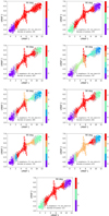 |
Fig. B.1. Bidimensional UMAP projection colour-coded according to HDBSCAN clustering applied to a ten-dimensional UMAP embdedding for the set of line-of-sight velocity maps of edge-on galaxies (Sect. 4.1). The outliers are shown as grey dots. Also included are the values of n_neighbors and min_dist, as well as the number of outliers. |
All Tables
Summary of the HDBSCAN clustering at different inclinations using the line-of-sight velocity maps.
Summary of the HDBSCAN clustering at different inclinations using the three types of kinematic maps.
Number of galaxies and repetitions in each group obtained when applying UMSCANGALACTIK to the mixture of the kinematic maps for the same galaxies observed at three different inclinations.
Analysis of the explained variance (% var) for two and ten principal components (PCs) and number of PCs needed to explain 75 per cent of the variance for the PCA algorithm applied to the sample of (a) line-of-sight velocity maps (Experiment 1) and (b) three types of kinematic maps (Experiment 2) for different inclinations.
All Figures
|
Fig. 1. Examples of line-of-sight velocity (left panels), dispersion (middle panels), and flux (right panels) maps for a galaxy with low rotation (upper panels), a clockwise rotating galaxy (middle panels), and an anticlockwise rotating galaxy (bottom panels). The maps are obtained from the kinematic data cubes generated by SIMSPIN by collapsing each data cube along the velocity axis, as described in Harborne et al. (2020). |
| In the text | |
|
Fig. 2. Results of UMSCANGALACTIK applied to the line-of-sight velocity maps of our galaxy sample at inclination 90 degrees. Top row: HDBSCAN clusters in the UMAP bidimensional projection. The outliers of the method are shown as grey dots (left panel), and distributions of the projected parameters ε (middle panel) and λR (right panel) on the projection. Second row: Size of the clusters (left panel), and PDFs of ε (middle panel) and λR (right panel) for each cluster. Third row: Distribution of three-dimensional parameters D/T (left panel), T (middle panel), and λB (right panel) on the projection. Bottom row: PDFs of D/T (left panel), T (middle panel), and λB (right panel) for each cluster. The colour bar limits are fixed to the 10th and 90th percentile of the variables. |
| In the text | |
|
Fig. 3. Results of UMSCANGALACTIK applied to the line-of-sight velocity maps in which every galaxy has the same rotation direction. Top panel: HDBSCAN clusters in the UMAP bidimensional projection. The outliers of the method are shown as grey dots. Bottom panel: Distribution of D/T on the projection. |
| In the text | |
|
Fig. 4. Analysis of the λR − ε plane. Left panel: λR − ε plane for the clustered galaxies. The symbols depicting clusters follow the colour-coding in Fig. 2. Middle panel: λR − ε plane for galaxies of C2 colour-coded by D/T. Right panel: λR − ε plane for galaxies of C0 and C1 colour-coded by D/T. The colour bar limits are fixed to the 10th and 90th percentiles of the variables. We include in all cases the criterion in Eq. (1) depicted by the black solid lines. |
| In the text | |
|
Fig. 5. Results of UMSCANGALACTIK applied to the line-of-sight velocity maps of our galaxy sample at different inclinations. Top panels: HDBSCAN clusters in the UMAP bidimensional projection of the line-of-sight velocity maps of galaxies observed at 60, 45, 30, and 20 degrees. The outliers of the method are shown as grey dots. Middle panels: Distributions of D/T on each projection. The colour bar limits are fixed to the 10th and 90th percentiles of the variables. Bottom panels: λR − ε plane. The symbols depict clusters following the same colour-coding as in the top panels. We include the criterion in Eq. (1) depicted by the black solid lines. |
| In the text | |
|
Fig. 6. Results of UMSCANGALACTIK applied to all kinematic map types of our galaxy sample at inclination 90 degrees. Top row: HDBSCAN clusters in the UMAP bidimensional projection. The outliers of the method are shown as grey dots (left panel), and distributions of the projected parameters ε (middle panel) and λR (right panel) on the projection. Second row: Size of the clusters (left panel), and PDFs of ε (middle panel) and λR (right panel) for each cluster. Third row: Distribution of three-dimensional parameters D/T (left panel), T (middle panel), and λB (right panel) on the projection. Bottom row: PDFs of D/T (left panel), T (middle panel), and λB (right panel) for each cluster. The colour bar limits are fixed to the 10th and 90th percentiles of the variables. |
| In the text | |
|
Fig. 7. Comparison between the clustering obtained using all kinematic map types and the line-of-sight velocity maps alone discussed in Sect. 4.1. Top panel: UMAP projection obtained from all kinematic maps according to the clustering obtained for the line-of-sight velocity maps, colour-coded as in Fig. 2. Bottom panel: Clustering in Fig. 6, repeated here for comparison. |
| In the text | |
|
Fig. 8. Results of UMSCANGALACTIK applied to all kinematic map types of our galaxy sample at different inclinations. Top panels: HDBSCAN clusters in UMAP bidimensional projection of the set of all kinematic maps of galaxies observed at 60, 45, and 30 degrees. The outliers of the method are shown as grey dots. Middle panels: UMAP projection obtained from all kinematic map types according to the clustering obtained for the line-of-sight velocity maps discussed in Sect. 4, colour-coded as in Fig. 5Bottom panels: Distributions of D/T on each projection. The colour bar limits are fixed to the 10th and 90th percentiles of the variables. |
| In the text | |
|
Fig. 9. Results of UMSCANGALACTIK applied to all the kinematic map types of galaxies with λR, edge − on ≤ 0.2 observed at 90 degrees. Top row: HDBSCAN clusters in the UMAP bidimensional projection. The outliers of the method are shown as grey dots (left panel), and distributions of the projected parameters ε (middle panel) and λR (right panel) on the projection. Second row: Size of the clusters (left panel), and PDFs of ε (middle panel) and λR (right panel) for each cluster. Third row: Distributions of three-dimensional parameters D/T (left panel), T (middle panel), and λB (right panel) on the projection. Bottom row: PDFs of D/T (left panel), T (middle panel), and λB (right panel) for each cluster. The colour bar limits are fixed to the 10th and 90th percentiles of the variables. |
| In the text | |
|
Fig. 10. Analysis of the 3D axis of galaxies with λR, edge − on ≤ 0.2. Top panels: Distributions of b/a (left panel) and b/a − c/a (middle panel) in the UMAP projection of the kinematic maps depicted in Fig. 9, and T vs b/a according to the clusters following the colour-coding in Fig. 9 (right panel). Bottom panels: PDFs of b/a (left panel) and b/a − c/a (middle panel), and T vs b/a for C0 colour-coded according to D/T (right panel). The colour bar limits are fixed to the 10th and 90th percentiles of the variables. |
| In the text | |
|
Fig. 11. Results of UMSCANGALACTIK applied to all the kinematic map types of galaxies with λR, edge − on > 0.2 observed at 90 degrees. Top row: HDBSCAN clusters in the UMAP bidimensional projection (left panel), and distributions of the projected parameters ε (middle panel) and λR (right panel) on the projection. Second row: Size of the clusters (left panel), and PDFs of ε (middle panel) and λR (right panel) for each cluster. Third row: Distributions of three-dimensional parameters D/T (left panel), T (middle panel), and λB (right panel) on the projection. Bottom row: PDFs of D/T (left panel), T (middle panel), and λB (right panel) for each cluster. The colour bar limits are fixed to the 10th and 90th percentiles of the variables. |
| In the text | |
|
Fig. 12. Results of UMSCANGALACTIK applied to all the kinematic map types of our galaxy sample mixing three different inclinations. Top row: HDBSCAN clusters in the UMAP bidimensional projection. The outliers of the method are shown as grey dots (left panel), and distributions of the projected parameters ε (middle panel) and λR (right panel) on the projection. Second row: Size of the clusters (left panel), and PDFs of ε (middle panel) and λR (right panel) for each cluster. Third row: Distributions of three-dimensional parameters D/T (left panel), T (middle panel), and λB (right panel) on the projection. Bottom row: PDFs of D/T (left panel), T (middle panel), and λB (right panel) for each cluster. The colour bar limits are fixed to the 10th and 90th percentiles of the variables. |
| In the text | |
|
Fig. A.1. λB as a function of ε where ellipticities are computed at different inclinations. The decrease in the values of ε with decreasing inclination indicates that galaxies are seen to be rounder when observed at low inclinations. |
| In the text | |
|
Fig. B.1. Bidimensional UMAP projection colour-coded according to HDBSCAN clustering applied to a ten-dimensional UMAP embdedding for the set of line-of-sight velocity maps of edge-on galaxies (Sect. 4.1). The outliers are shown as grey dots. Also included are the values of n_neighbors and min_dist, as well as the number of outliers. |
| In the text | |
Current usage metrics show cumulative count of Article Views (full-text article views including HTML views, PDF and ePub downloads, according to the available data) and Abstracts Views on Vision4Press platform.
Data correspond to usage on the plateform after 2015. The current usage metrics is available 48-96 hours after online publication and is updated daily on week days.
Initial download of the metrics may take a while.