| Issue |
A&A
Volume 670, February 2023
|
|
|---|---|---|
| Article Number | A126 | |
| Number of page(s) | 22 | |
| Section | Interstellar and circumstellar matter | |
| DOI | https://doi.org/10.1051/0004-6361/202141664 | |
| Published online | 17 February 2023 | |
Forbidden emission lines in protostellar outflows and jets with MUSE
1
Max Planck Institut für Astronomie,
Königstuhl 17,
69117
Heidelberg, Germany
e-mail: This email address is being protected from spambots. You need JavaScript enabled to view it.
2
Department of Physics, Texas State University, San Marcos,
601 University Dr,
San Marcos, TX
78666, USA
3
Institutionen för astronomi, Stockholms universitet, AlbaNova universitetscentrum,
106 91,
Stockholm, Sweden
4
Astrophysics Research Institute, Liverpool John Moores University, IC2,
Liverpool Science Park, 146 Brownlow Hill,
Liverpool,
L3 5RF, UK
5
School of Physics, University College,
Belfield, Dublin 4, Ireland
6
Fakultät für Physik, Universität Duisburg-Essen,
Lotharstraße 1,
47057
Duisburg, Germany
7
Institut für Astronomie und Astrophysik, Universität Tübingen,
Auf der Morgenstelle 10,
72076
Tübingen, Germany
8
Physikalisches Institut, Universität Bern,
Gesellschaftsstr. 6,
3012
Bern, Switzerland
9
Instituto de Radioastronomía y Astrofísica(IRyA),
Universidad Nacional Autónoma de México (UNAM),
Mexico
10
Institute for Advanced Study, Tsinghua University,
Beijing
100084, PR China
Received:
29
June
2021
Accepted:
19
December
2022
Abstract
Context. Forbidden emission lines in protoplanetary disks are a key diagnostic in studies of the evolution of the disk and the host star. They signal potential disk accretion or wind, outflow, or jet ejection processes of the material that affects the angular momentum transport of the disk as a result.
Aims. We report spatially resolved emission lines, namely, [O I] λλ6300, 6363, [N II] λλ6548, 6583, Hα, and [S II] λλ6716, 6730 that are believed to be associated with jets and magnetically driven winds in the inner disks, due to the proximity to the star, as suggested in previous works from the literature. With a resolution of 0.025 × 0.025 arcsec2, we aim to derive the position angle of the outflow/jet (PAoutflow/jet) that is connected with the inner disk. We then compare it with the position angle of the dust (PAdust) obtained from previous constraints for the outer disk. We also carry out a simple analysis of the kinematics and width of the lines and we estimate the mass-loss rate based on the [O I] λ6300 line for five T Tauri stars.
Methods. Observations were carried out with the optical integral field spectrograph of the Multi Unit Spectroscopic Explorer (MUSE), at the Very Large Telescope (VLT). The instrument spatially resolves the forbidden lines, providing a unique capability to access the spatial extension of the outflows/jets that make the estimate of the PAoutflow/jet possible from a geometrical point of view.
Results. The forbidden emission lines analyzed here have their origin at the inner parts of the protoplanetary disk. From the maximum intensity emission along the outflow/jet in DL Tau, CI Tau, DS Tau, IP Tau, and IM Lup, we were able to reliably measure the PAoutflow/jet for most of the identified lines. We found that our estimates agree with PAdust for most of the disks. These estimates depend on the signal-to-noise level and the collimation of the outflow (jet). The outflows/jets in CIDA 9, GO Tau, and GW Lup are too compact for a PAoutflow/jet to be estimated. Based on our kinematics analysis, we confirm that DL Tau and CI Tau host a strong outflow/jet with line-of-sight velocities much greater than 100 km s−1, whereas DS Tau, IP Tau, and IM Lup velocities are lower and their structures encompass low-velocity components to be more associated with winds. Our estimates for the mass-loss rate, Ṁloss, range between (1.1–6.5) × 10−7–10−8 M⊙ yr−1 for the disk-outflow/jet systems analyzed here.
Conclusions. The outflow/jet systems analyzed here are aligned within around 1° between the inner and outer disk. Further observations are needed to confirm a potential misalignment in IM Lup.
Key words: line: profiles / protoplanetary disks / stars: jets / line: identification
© The Authors 2023
 Open Access article, published by EDP Sciences, under the terms of the Creative Commons Attribution License (https://creativecommons.org/licenses/by/4.0), which permits unrestricted use, distribution, and reproduction in any medium, provided the original work is properly cited.
This article is published in open access under the Subscribe to Open model.
Open Access funding provided by Max Planck Society.
1 Introduction
The detection of forbidden emission lines in different samples of T Tauri stars has provided access to different physical conditions depending on their line-of-sight (LoS) velocity information. Line decomposition methods have led to the classification of different velocity components that originate from different physical mechanisms (Hamann 1994; Hartigan et al. 1995; Ercolano & Pascucci 2017; Fang et al. 2018; Banzatti et al. 2019; Pascucci et al. 2020). Outflows, jets, magnetospheric accretion, and disk winds influence the angular momentum transport (i.e., Casse & Ferreira 2000; Casse & Keppens 2002; Sheikhnezami et al. 2012; Stepanovs & Fendt 2016). In most of the disk regions, the magneto-rotational instability (MRI; Balbus & Hawley 1991) is almost entirely suppressed by non-ideal magnetohydrodynamic (MHD) effects (Bai & Stone 2013) because of the low level of coupling between the gas and the magnetic field. At the same time, strong magnetic fields give rise to magnetically driven winds (Blandford & Payne 1982), as in the uppermost layers of the disk atmosphere, the gas and magnetic field are coupled again. On the other hand, thermal photoevaporative winds can co-exist with magnetically driven winds (Rodenkirch et al. 2020). In the regions where thermal disk winds are generated, the surrounding gas must be highly ionized at least enough for electrons to be thermally excited; temperatures can be greater than 5,000 K with gas densities between 105–106 cm−3 (Simon et al. 2016). Therefore, studying forbidden emission lines can provide clues about the main processes taking place in the inner disk.
T Tauri sources show complex velocity line profiles. The low-velocity component (LVC) can be classified in two components: the narrow component (NC) and the broad component (BC); both presumably tracing photoevaporative or magnetohydrodynamic winds. Whelan et al. (2021) reported the first detection of MHD winds, which spatially resolved the forbidden emission lines using spectroastrometry analysis. On the other hand, a small percentage (~30%; Nisini et al. 2018) shows a high-velocity component (HVC) associated with jets. Though different mechanisms form winds and outflows and jets, collimated disk winds could form the base of an outflow-like or jet-like structure. Many surveys (i.e., Hamann 1994; Hartigan et al. 1995; Hirth et al. 1997; Antoniucci et al. 2011; Rigliaco et al. 2013; Natta et al. 2014; Simon et al. 2016; Nisini et al. 2018; Fang et al. 2018; Banzatti et al. 2019) have shown that the HVC of the [O I] λ6300 excitation line is common and likely probing outflows, jets, or MHD winds (Edwards et al. 1987; Hartigan et al. 1995; Bacciotti et al. 2000; Lavalley-Fouquet et al. 2000; Woitas et al. 2002). Moreover, the HVC in T Tauri disks has been spatially confirmed to be associated with jets. Their emission reaches a greater extension from the star than those lines with the LVC (Dougados et al. 2000). Other lines, such as [N II] λ6583 and [S II] λ6731, have also been reported to probe outflows and jets (Solf & Boehm 1993; Dougados et al. 2000; Lavalley-Fouquet et al. 2000; Woitas et al. 2002; Natta et al. 2014; Nisini et al. 2018), in which the detailed kinematic structure has been determined from the analysis of such intrinsic line profiles. Another important line is Hα, which also traces the velocity fields of outflows and jets (Edwards et al. 1987; Bacciotti et al. 2000; Woitas et al. 2002), as well as accretion processes in the accretion flow onto a planet and in the circumplanetary disk (i.e., Haffert et al. 2019; Hashimoto et al. 2020; Marleau et al. 2022).
Studying the connection between the inner and outer disk has attracted much attention lately. Despite the rings and gaps seen in protoplanetary disks, shadows could indicate some degree of misalignment between the inner and outer disk (Marino et al. 2015; Stolker et al. 2016; Min et al. 2017; Debes et al. 2017; Benisty et al. 2017, 2018; Casassus et al. 2018; Pinilla et al. 2019; Muro-Arena et al. 2020). Resolving the inner parts of the disk is quite challenging. A recent study by Bohn et al. (2022) showed that it is possible to assess the inner disk using near-infrared and submillimeter observations in T Tauri and Herbig Ae/Be disks. They emphasize the difficulty of measuring a possible misalignment between inner and outer disks in T Tauri disks, mainly due to the limited angular resolution of VLT/GRAVITY or the specific geometry orientation of the disks.
In this paper, we introduce the detection of forbidden emission lines such as: [O I] λλ6300, 6363, [N II] λλ6548, 6583, Hα, and [S II] λλ6716, 6730 for the first time in some T Tauri sources with the MUSE/VLT instrument in the narrow-field mode (NFM). These forbidden emission lines originate from the innermost part of the disk as outflows/jets and we estimate the position angle (PAoutflow/jet) that is connected with the inner disk and compare it with the dust position angle (PAdust), derived from previous work. In Sect. 2, we describe the physical properties of the disk using the Atacama Large Millimeter/submillimeter Array (ALMA) and the MUSE observations. In Sect. 3, we present our estimates of the PAoutflow/jet and analyze the velocity components from the line profiles. In Sects. 4 and 5, we present our summary and conclusions, respectively.
2 Disk parameters and observations
We briefly summarize the disk observational description of the dust continuum emission. The physical properties we use to compare the properties of the outflows/jets are originally constrained by previous studies. Lastly, we introduce the MUSE observations.
2.1 Dust continuum parameters
The disks presented here have been well studied and are known to have dust substructures detected at millimeter wavelengths. We adopted some additional disk properties, such as the inclination and PAdust, from previous work that performed the disk model fitting based on the dust morphology and the origin of the substructures. The distance of each source is obtained from the Gaia Collaboration (2021).
The disk properties were obtained and analyzed from three different datasets. The disk properties from IM Lup and GW Lup were obtained from the Disk Substructures at High Angular Resolution Project (DSHARP) at 1.25 mm continuum observations with a high spatial resolution of 0704 (Andrews et al. 2018; Huang et al. 2018). For the disks in the Taurus star-forming region, we considered the ALMA Cycle 4 observations (ID: 2016.1.01164.S; PI: Herczeg) that were observed at 1.33 mm and a resolution of ~0″.12 (Long et al. 2018, 2019).
2.2 MUSE observations and data reduction
The observations were carried out between November 2019 and January 2020 with VLT/MUSE in the NFM under program-ID 0104.C-0919 (PI: A. Müller). The MUSE optical integral field spectrograph covers the spectral range from 4650–9300 Å at a resolving power of ~2000 at 4600 Å and ~4000 at 9300 Å (Bacon et al. 2010), with a spectral sampling of 0.125 nm per pixel. The adaptive-optics assisted NFM has a field of view (FOV) of 7.4×7.4 arcsec2 with a spatial scale of 0.025 arcsec per pixel, which is a pixel scale that is about ten times smaller than the wide-field mode. With this spatial resolution, we can recover the spatial extension, by means of x and y pixels, of the emission coming from the outflows/jets. The VLT adaptive optics system uses four laser guide stars whose wavelengths range from 5781 Å to 6048 Å. This spectral range is removed from the MUSE spectra to avoid the presence of additional lines that occur when the laser interacts with air molecules.
The MUSE-NFM observations were reduced with the standard ESO pipeline v2.8.1 (Weilbacher et al. 2012, 2014, 2016), which includes bias subtraction, spectral extraction, flat-fielding, wavelength calibration, and flux calibration. Although the NFM includes an atmospheric dispersion corrector (ADC), the centroid variations can still be a few spatial pixels along the entire wavelength range. Therefore, we corrected the calibrated pixel tables for each exposure based on the centroid shifts with wavelengths measured on intermediate cube reconstructions. The corrected pixel tables were then used to create the combined cube of all calibrated exposures.
The wavelength calibration was done using a helium-argon ARC lamp from the day before each night of observations. Due to temperature variations, the wavelength solution for a given spectrum can be offset and an empirical wavelength correction using bright skylines should be applied (Weilbacher et al. 2020). Skylines are, however, faint in the NFM, so this wavelength correction is hard to apply. These offsets can vary from target to target and are on the order of fractions of a pixel, up to a full pixel in extreme cases (5–50 km s−1; see also Xie et al. 2020). We report eight data cubes that were obtained over 0.5 h each.
2.3 MUSE and ALMA image registration
When comparing the MUSE images with ALMA data, we focus on comparing the geometry of the dusty outer disk plane, as measured with ALMA, and the position angle of the outflows/jets, as measured with MUSE. With the assumption that the disk is circular and the star is at its center, the ALMA observations can be used to recover the inclination and the position angle relative to the fitted disk center. In our sample, the systems have their disk geometry calculated through visibilities (Long et al. 2018) or image fitting (Huang et al. 2018), and we adopted those published values for our inclination and position angle for the outer disk plane. As both works fit the center of the disk under the assumptions mentioned above, the PAdust already includes the observational and instrumental uncertainties, which remain fixed in this work.
With MUSE, our assumption to recover the PAoutflow/jet is that the star is centered in the image frame. In order to confirm this, we fit a 2D circular Gaussian to the specific channels we used to analyze the PAoutflow/jet. We do this to the reduced data cube without PSF subtraction, assuming that the outflow/jet emission is negligible compared to the stellar emission. We found that for each channel, the center of the Gaussians is less than 1 pixel (or smaller than 25 mas) from the center of the images for all sources. Therefore, we measured the PAoutflow/jet relative to the center of the image where the star is.
When comparing ALMA with MUSE, the assumptions are that the outer disk geometry (incl, PAdust) was measured relative to the same point as the PAoutflow/jet, which is the stellar position. Additionally, the outer disk plane did not change even when both images were taken at different epochs. The comparison of the geometry of the disk with different instruments is similar to the work done by Bohn et al. (2022), where they combined the K-band from GRAVITY/VLTI to constrain the geometry of the inner disk by finding the best parametric SED solution to the squared visibilities. These authors used ALMA 12CO and 13CO data to constrain the geometry of the outer disk. Their determination of potential misalignment between the inner and outer disks is narrowed down by comparing the inclinations and position angles defined by the planes of the inner and outer disks, respectively. The GRAVITY Collaboration (2020) describes the position angle constrained by ALMA to be a well-fixed parameter in order to describe the geometry of the disk. We include the rotational accuracy as 0.2° when propagating the uncertainty for each PAoutflow/jet value in Table 1 (see also Appendix D).
3 Results
We identified seven forbidden emission lines: [O I] λλ6300, 6363, [N II] λλ6548, 6583, Hα, [S II] λλ6716, 6730, which are seen to be originating from the innermost part of the disk as outflow-like or jet-like structures (Figs. 1, C.2, E.1, E.2, and E.3). Some of these lines have been reported in some of the sources we analyzed here (i.e., Simon et al. 2016; Fang et al. 2018; Banzatti et al. 2019). We used Natta et al. (2014), Podio et al. (2006), and the NIST atomic spectra database for the line identification and line uncertainty. The PAoutflow/jet is defined as the position angle of the outflow/jet measured in degrees that lie approximately in the direction perpendicular to the rotational axis of the disk. In the next section, we detail how the geometrical derivation of the PAoutflow/jet is conducted. It is very likely that we are not solely seeing jets, but also outflows and (perhaps) winds that cannot be revealed due to the low spectral resolution of MUSE. Any description and analysis of winds are out of the scope of the present work, as it is necessary to assess the few km s−1 velocity components that characterize them. We performed a Gaussian fit to the emission lines to study their velocity components and, finally, we measured the length of the outflow/jet to estimate the mass loss from the [O I] λ6300 line.
3.1 Geometrical fitting of the outflows/jets
In order to derive the PAoutflow/jet for each spectral line in all disks, we fit the jet intensity peaks with a linear function (after stellar subtraction). We read the maximum value across the outflow/jet for the forbidden emission lines detected on each source and store the x and y positions corresponding to the jet emission into a new array. These are then converted into polar coordinates, where  and θ = arctan(y/x). Jet intensity peaks are only considered if they are above 5σ of the background. For other imaging parameters and wavelengths (see Table B.1 and F.1). The retrieved positions contain the angular information to calculate the PAoutflow/jet. In order to fit a line along these retrieved positions of the jet, we employed a fitting method called the orthogonal distance regression (ODR; Brown et al. 1990). This routine gathers the retrieved data and the linear model function to produce the best linear parameters for the jet. The linear model function follows the simple ordinary prescription of a line, f(xi;β) = β1 x + β0, where, xi is the position in pixels, and β0 and β1 are the unknown parameters to be found by the ODR routine. We assign an initial standard deviation for each jet peak position to be 1 pixel. Choosing a value of 1 pixel is a conservative selection for the initial standard error as we found that when estimating the PAoutflow/jet, the corresponding error of the Gaussian center is smaller than 1 pixel. As the function we used for the fit, f(xi; β), is said to be linear in variables, xi, and linear in parameters, β, the total error in the routine is estimated by applying the linear least squares method. That is, by finding the set of parameters for which the sum of the squares of the n orthogonal distances from the f(xi; β) curve to the n data points is minimized. This error associated at the end of the fit follows: min
 ![Mathematical equation: $\sum\nolimits_{i = 1}^n {{{\left[ {{y_i} - f\left( {{x_i} + {\delta _i};{\bf{\beta }}} \right)} \right]}^2} + \delta _i^2} $](/articles/aa/full_html/2023/02/aa41664-21/aa41664-21-eq2.png) , where δi is the error associated to each n data point.
, where δi is the error associated to each n data point.
For the iterative routine to estimate the PAoutflow/jet for each emission line, we used (as an initial estimate) the PAoutflow/jet from the locations of the jet intensity peaks from the first part. Then, we used this first value for the PAoutflow/jet as a seed for a second iteration, where we fit Gaussians to profiles that are orthogonal to the jet axis defined by the first PAoutflow/jet. Depending on the source, the first three to five pixels were not used to avoid artifacts from the stellar subtraction at the image center. For example, a comparison between the peak intensity locations and the Gaussian centers is shown for DL Tau in Fig. A.2. Those Gaussian centers were then used to calculate the final PAoutflow/jet for each emission line. The final PAoutflow/jet of the disks for which we detect bright emission lines are shown in Table 1. Then, we took the average, PAoutflow/jet, from the PAoutflow/jet estimates of different emission lines in Table 1 and we added the corresponding errors in quadrature. This  value for each source was then used to compared with the PAdust (see Table 2). We note that the CIDA9, GO Tau, and GW Lup jets were too compact at the center, making it difficult to properly estimate any PAoutflow/jet. Before making the comparison between the
  and the PAdust, it is important to understand the side of the disk plane which the emission line is coming from. We used the same geometrical convention as in Fig. 3 from Piétu et al. (2007) to indicate the real disk plane configuration through the inclination for each disk system.
In Fig. 2, we portray this convention by superimposing the outflows/jets to the mm dust continuum of the protoplanetary disk. It shows a better visualization of the measured  , in comparison with the PAdust, for DL Tau (left panel) for the negative outer disk inclination case, and CI Tau (right panel) for the positive outer disk inclination case. DS Tau, IP Tau, and IM Lup have negative outer disk inclinations. The PAdust follows the usual standard definition of the position angle of the major axis of the outer disk, from 0° to 180°, from north to east. Since DL Tau has a negative outer disk inclination, the PAoutflow/jet values are measured counterclockwise from the north, and it is similar to saying that the disk is flipped. On the other hand, CI Tau has a positive outer disk inclination then the PAoutflow/jet values are measured clockwise from the north. Having identified the orientation of the outer disk inclination, we determined the rotation of the protoplanetary disk-outflow/jet system (see Fig. C.2).
We took into account the difference between the PAoutflow/jet, which is related to the PA of the innermost disk, and the PAdust. For this, we followed:
 (1)
(1)
We found that the difference between the  and the PAdust to be small in general (see Table 2). For the sources analyzed here, the estimation of the PAoutflow/jet and their associated errors lie within the estimation of the PAdust and its associated error range. Under the assumption that the outflow (or jet) axis is perpendicular to the inner disk plane, we do not find any misalignment between the inner and outer disk. The spread of the PAoutflow/jet values in Table 1 depend on the uncertainties and values coming from the Gaussian fit centers. The symmetric Gaussian fit model is not well suited to capture possible asymmetries in outflows/jets produced by low signal-to-noise variations, especially close to the center of the images where the rms is not constant (see Fig. 3). Our rms values are estimated in a region free from stellar and outflow/jet emission; however, the rms value close to the image center is not constant due to contamination when subtracting the stellar spectrum. Those effects are not systematically considered in our PAoutflow/jet estimates, therefore, our uncertainties should be considered as lower limits. It is the case that the estimation of the PAoutflow/jet for IM Lup was more difficult because of its compact extent and low signal-to-noise level. The intensity variations in the outflow/jet are comparable to noise variation level, resulting in a PAoutflow/jet difference of 6° between the [O I] λ6300 and [N II] λ6583 lines. By calculating the difference between PAoutflow/jet and PAdust we get 5.18° ± 1.77° and 0.94° ± 1.08° for [O I] λ6300 and [N II] λ6583 line, respectively. The
  and PAdust are different by 2.12° ± 1.99°, therefore, the difference is within the uncertainty. This is further discussed in Sect. 4.
Overall, we detected two essential geometrical features. One is a broadening of the respective intensity distribution with distance, indicating that the jet width increases with distance from the star. The other feature is the variation of the location of the intensity maximum, indicating a wiggling of the jet axis. A periodic pattern in these changes may hint at a precession or orbiting jet (Fendt & Zinnecker 1998). In Fig. 3, the wiggle patterns are marked by the Gaussian centers as navy color dots. We further investigate how these Gaussian centers vary in position with respect to their distance from the jet axis (see Fig. A.1 and Fig. A.2). In order to check whether or not these successive Gaussian centers have periodicity, we calculate their deviation of them from the jet axis. Applying a simple sinusoidal function in a periodogram does not provide significance, even if essentially done by eye – as there seems to be some quasi-periodic behavior in the Gaussian centers. In Sect. 4, we further discuss how the patterns of the Gaussian centers could possibly hint at a sign of jet precession.
Outflow/jet properties.
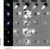 |
Fig. 1 Composite image of different protoplanetary disks at four different forbidden emission lines. First column shows the dust continuum emission at 1.3 mm from ALMA cycle 4 (Long et al. 2018, 2019). Other columns show the different forbidden emission lines from MUSE as labeled in the top left of the first row. Dashed yellow rectangles mark the area from where we gather the spectrum of the jet by summing over the spatial axes within the dashed yellow frame of the image. |
Disk properties (geometric parameters).
3.2 Outflow/jet velocities
The emission of these forbidden optical emission lines has been established to trace outflows/jets and winds in T Tauri stars. From their line velocity, we can characterize whether it is a high-velocity or a low-velocity component (Edwards et al. 1987; Hartigan et al. 1995). For each spectral frame in the data cube, we summed pixel fluxes over the region defined by the dashed yellow rectangles in Fig. 1 to obtain a spectrum of the emission. To measure the emission line centroids to sub-pixel precision, we take the line peak from a Gaussian fit to the data (see Figs. 4,5,6, and 7). In Table 1, we report the de-projected outflow/jet velocities estimated from the Gaussian fits as follows: υoutflow/jet = c ((λgauss – λref)/λref) / cos(incl), where c is the speed of light, incl is the inclination of the disk (Table 2), λgauss is the Gaussian fit centroid, and λref is the rest wavelength of each forbidden line in the air. The errors on the de-projected velocities, υoutflow/jet, in Table 1 are propagated from the Gaussian fit and the disk inclination, but do not include the uncertainty in wavelength calibration that is likely between 5 km s−1 up to 50 km s−1 (see Xie et al. 2020). Most of the υoutfloe/jet that we could estimate from the emission lines are blue-shifted and their values correspond mostly (but are not limited to) to the high-velocity components. We determine that for each source, we only see one side of the outflow/jet and the dust from their protoplanetary disk obscures the receding part of these outflow/jet velocities. Unlike the onesided blue-shifted sources, we report the red-shifted velocities for DS Tau.
The detection of Hα line seems to stand out in the spectra (Figs. E.1, E.2, and E.3). However, the Hα emission is seen spread in an area surrounding the line spread function, similar to a high noise intensity that Hα introduces from a high photon count level. This effect is not necessarily seen prominently in DL Tau (Fig. 4). An instrumental artifact causes this spread and the reason behind this effect is unknown. Similar effects have been seen and analyzed by Xie et al. (2020), where the Hα line-to-continuum ratio varies across the field. These variations are so high that the residuals due to this instrument issue are stronger than those from photon noise. The noise reduction is taken into account when applying the principal component analysis (PCA; Soummer et al. 2012) method, but the error scale is so high that quantifying the real emission of Hα over the area is difficult.
The structured spectral line profiles reported here show the intrinsic outflow/jet velocity peaks or the line-of-sight velocity for the lines that we were able to capture in the spectra (Figs. 4, 5, 6, and 7). The velocity values reported here are corrected with the stellar radial velocity that is reported in Table 2 from both Banzatti et al. (2019) and Fang et al. (2018). The [O I] λ6300, Hα, [N II] λ6583, and [S II] λ6730 line profiles (Figs. 5, 6, and 7) for DL Tau and CI Tau are considerably blue-shifted with line center velocities much greater than 100 km s−1. The deprojection velocities show that the velocity of the outflow/jet, υoutflow/jet, for DL Tau and CI Tau are greater or very close to 200 km s−1 tracing strong outflows/jets, as shown in see Table 1. Highresolution spectra for DL Tau have shown a single low-velocity and a high-velocity component (Banzatti et al. 2019). The highvelocity component dominates the MUSE image. In addition, DL Tau hosts the most extended and collimated outflow/jet, reaching approximately 180 AU. For CI Tau, a strong outflow/jet is reported for the first time: its morphology is different from the DL Tau one, as seen in Fig. 2 (right panel). By taking 200 km s−1 as an approximate velocity of the jets in DL Tau and CI Tau, and a distance of 159 pc and 160 pc, respectively, then the proper motion of their extended outflow/jet is about 0″.26 per year.
The emission lines of DS Tau, IP Tau, and IM Lup have rather minor line-of-sight velocity shifts of less than 100 km s−1 (except for DS Tau) and broader line widths considerably overlapping 0 km s−1, which could hide some LVC emission. DS Tau is the only source in this sample where the line emission appears red-shifted rather than blue-shifted. This red-shifted emission is consistent with a high disk inclination (see Table 2) observed with ALMA, where the outflow/jet appears only from the back side of the disk (see Fig. C.2). The IP Tau disk is a transition disk as seen in mm continuum emission (Long et al. 2018). The MUSE data for IP Tau shows a blue-shifted component in the [Ol] λ6300 line with properties in between the HVC and the LVC, which is in good agreement with what has been observed in high-resolution spectral analysis (Banzatti et al. 2019). Interestingly, this line has been reported to vary over time (Simon et al. 2016). A recent work by Bohn et al. (2022) found no potential misalignment between the inner and outer disk in IP Tau when analyzing the VLT/GRAVITY and ALMA data. IM Lup is known to have a blue-shifted LVC- BC measured from the [O I] λ6300 line (Fang et al. 2018).
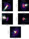 |
Fig. 2 Visualization of the estimated |


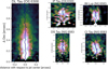 |
Fig. 3 Successive Gaussian centers shown as navy-colored dots. Wiggles are seen in DL Tau and IP Tau at [O I] λ6300, and for CI Tau, DS Tau, and IM Lup at [N II] λ6583. |
 |
Fig. 4 Hα line profile identified for DL Tau probing the high line-of-sight velocity component coming from the strong outflow/jet. The red dashed line represent the line-of-sight maximum velocity. |
3.3 Are emission lines resolved?
We have classified whether or not the emission lines we report are resolved, marginally resolved, or unresolved (see Table F.1), depending on the resolution limit that MUSE has at the wavelength of a given emission line (Fig. 8). Resolving the line width implies that the emission line width is larger than the line-broadening of MUSE. The [S II] λ6716 line, for example, is marginally equal to the line-broadening FWHM of MUSE (115 km s−1) in DL Tau (Fig. F.1); but in CI Tau, it is resolved given that the measured width is approximately 150 km s−1 (see Fig. F.2), which is greater than the instrumental resolution. Marginally resolved lines and unresolved lines, in particular, should be considered to upper limits rather than precise estimates of the emission line widths (i.e., Eriksson et al. 2020). The Hα line in almost all samples, except in CI Tau, is mostly unresolved because their measured width is less than the line-broadening FWHM of MUSE at Hα (119 km s−1). The spectral capability of MUSE has enabled to solve for the velocity components of the forbidden emission lines, leading to a good venue for the exploration of the momentum transport of the disk as the disk losses mass, in which such estimate depends on the line profile and the resolution limit of the instrument.
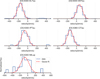 |
Fig. 5 [O I] λ6300 line proflies identified in five sources from our sample. DL Tau and CI Tau have their line centered at velocities greater than 100 km s−1, which is characteristic of jets. Unlike DL Tau and CI Tau, the disks of DS Tau, IP Tau, and IM Lup show smaller shifts of less than 100 km s−1 and broader line widths significantly overlapping with 0 km s−1, possibly including the LVC emission as a result. DS Tau has the most centered line. |
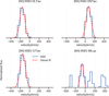 |
Fig. 6 [N II]/λ6583 line profiles identified in four sources from our sample. Same case as in Fig. 5, DL Tau and CI Tau probe high-velocity components, while DS Tau and IM Lup are more centered to zero. |
3.4 Mass-loss rate
The mass-loss rate considers the velocity and the length from the bright [O I] λ6300 line luminosity of the densest bulk of the outflow/jet. The [O I] λ6300 line is optically thin and used to trace the total mass in the outflow/jet (Hartigan et al. 1994; Giannini et al. 2015; Nisini et al. 2018; Fang et al. 2018). The mass-loss rate is:
 (2)
(2)
where V⊥ is the outflow/jet velocity that is deprojected from the LoS (see Table 1). The length of the outflow/jet is l⊥ = dpc θ, where dpc is the distance of the source given in Table 2, and θ is the length of the outflow/jet measured in arsec (see Tables B.1 and 3). The length of the outflow/jet is measured until the emission flux drops below 10−17 erg s−1 cm−2 Å−1. C(T, ne) is a coefficient of the [O I] λ6300 line transition from the energy state 2 → 1, that depends on the gas temperature via thermally excited collisions of electrons. At T = 10, 000 K, we used C(T, ne) = 9.0×10⁻⁵ for a ne = 5.0×104 cm−3, both values provided by Fang et al. (2018). The resulting mass-loss rates of the disk-outflow/jet sources are listed in Table 3. These mass-loss rates range (1.1–6.5)×10−7–10−8 M⊙ yr−1, which is in agreement with values reported by Hartigan et al. (1994, 1995); Nisini et al. (2018); Fang et al. (2018). A good advantage of the MUSE data is that the spatial extension of the outflow/jet can be measured. We use the distances of the sources specified in Table 2 to convert from angular length (arcsecs) to physical length (au). We adopted the same scaling distance as in Fang et al. (2018) at 100 au as a normalization factor of the extension of the outflow/jet. As noted, the mass-loss rate is proportional to the line luminosity of [O I] λ6300, which assumes a low electron number density that is much lower than the critical density (nH ~106 cm−3) and an atomic abundance similar to the standard interstellar medium (~10−4).
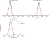 |
Fig. 7 [SII] λ6730 line profile identified for DL Tau, CI Tau, and DS Tau. |
3.5 Outflow/jet width in DL Tau
Figure 9 shows the width of six emission lines of the outflow/jet in DL Tau. The intensity profiles are compiled by stacking the Gaussian fits of the intensity slices across the outflow/jet as a function of the distance from the outflow/jet axis. The outflow/jet widths in Fig. 9 represent the average length, namely ~0″.5, of the extension of the outflow/jet in DL Tau. We converted the width of the outflow/jet) from pixels using the MUSE spatial resolution of 0/025 per pixel to angular distance: [O I] λ6300 = 0″.16, [O I] λ6363 = 0″.12, [N II] λ6583 = 0″.11, [S II] λ6716 = 0″.31, [S II] λ6730 = 0″.21, and Hα =0″.17. Each emission line width in au is shown in the legend box. The only emission line that is not included in the [N II] λ6548 line because it is very faint.
Each line profile traces different layers of the outflow/jet. The [O I] λ6363 line and the [N II] λ6583 line share very similar narrow widths and, compared to the other lines, they both seem to trace the deepest layer of the outflow (jet). These two lines also have similar FWHM (see Table 1), encouraging further studies to see whether [O I] λ6363 and the [N II] λ6583 could perhaps share the same physical properties of the emitting area. Interestingly, we see similar widths for Hα and [O I] λ6300. On the other hand, we found [S II] λ6716 to be the broadest line, followed by [S II] λ6730 line.
The brightest and most detected lines are [O I] λ6300 and [N II] λ6583 as a result of collisional excitation of electrons in shock fronts. The [S II] λ6716/[S II] λ6730 and [N II] λ6583/[O I] λ6300 line ratio can help to estimate the physical conditions concurring in these scenarios. Empirical fittings (Proxauf et al. 2014; Ellerbroek et al. 2014) and shock model analysis (Hartigan et al. 1994) suggest that these two line ratios are coming from regions with electron densities, ne, ranging from 103 to 104 cm−3, ionization fractions ranging from 0.2 to line ratio in the LVC emitting region have determined that these are emitted in rather dense gas (ne ≥ 107 cm−3), where the gas density relative to hydrogen, nH, is ≥1010 cm−3. In temperatures between 5000 and 104 K, these estimations are based on models where the excitation energies are due to collisions of electrons in regions dominated by neutral Hydrogen (Natta et al. 2014; Simon et al. 2016; Fang et al. 2018). Lavalley-Fouquet et al. (2000) mention that from the [N II] λ6583/[O I] λ6300 the line ratio diagnostic, the ratio increases with ionization fraction, in regions where ne ≥ nH. Lavalley-Fouquet et al. (2000) also stated that the [S II] λ6716 and [S II] λ6730 line ratio is a well-known decreasing function of the electronic density until ne ≥ ncr ~ 104 cm−3, the critical density for collision with electrons of [S II]. We encourage further analysis of the line ratio of these forbidden emission lines to the gas temperature, gas density, electron density, and ionization fraction that is characteristic depending on the region of the emitting area.
Mass-loss rates for the disk-outflow/jet systems.
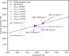 |
Fig. 8 Spectral resolution, R = λ/Δλ, versus wavelength of the seven forbidden emission lines used in the analysis here. The blue curve shows the resolution curve of MUSE at increments of 500 Å. Each R value for each line is linearly interpolated from the MUSE resolution curve. The values were obtained from the MUSE User Manual (version 11.4, Fig. 18). |
4 Discussion
The forbidden emission lines analyzed here originate from the center of the protoplanetary disks. Their shape indicates the presence of outflow/jet systems tracing the ongoing process of mass accretion to the star and mass extraction from the inner disk. A full analysis of the mass accretion from the lines is out of the scope of the current work. However, we are motivated to continue this analysis and compare the kinematics with the relative flux between HVC and LVC, with high-resolution spectra from Banzatti et al. (2019).
From the eight T Tauri systems, the averaged position angle of the outflow/jet,  , for DL Tau, DS Tau, CI Tau, IP Tau, and IM Lup (see Table 2) show no tendency of misalignment between the inner disk and the outer disk. The outflows/jets with low signal-to-noise levels and compact extensions close to the image center are challenging to the Gaussian fit method. Due to these effects, the orthogonal profiles of the outflow/jet can take non-Gaussian shapes which, combined with the variable rms in the image center, produce a systematic underestimation of the PAoutflow/jet uncertainties. For IM Lup, determining a PAoutflow/jet from the [O I] λ6300 and [N II] λ6583 lines was challenging due to the systematic issues mentioned resulting in a ΔPAoutflow/jet = 6° between the two emission lines. However, the PAoutflow/jet values from [O I] λ6300 and from [N II] λ6583 are tracing the same physical outflow/jet axis. The PA average of both emission lines for IM Lup are within the uncertainty range, therefore, no misalignment is detected between the inner and outer disk. However, we encourage follow-up observations with higher signal-to-noise to improve the PAoutflow/jet estimates for IM Lup. If there was a misalignment between the inner and outer disk, it would be an order of magnitude smaller than the reported values on other sources: 72° for HD 100453 (Benisty et al. 2017), 30° for HD14306 (Benisty et al. 2018), 30° for DoAR 44 (Casassus et al. 2018), and 70° for HD 142527 (Marino et al. 2015). One piece of observational evidence supporting the determination of no misalignment in IM Lup is the lack of shadows in scattered light (Avenhaus et al. 2018). For IP Tau, our result of no misalignment agrees with what has been found by Bohn et al. (2022) when performing a parametric model fit to the squared visibilities. The estimation of the PAoutflow/jet for different emission lines is a reliable way to illustrate the orientation of the inner disk and compare it to the PAdust. The two most detected lines in our sample are [O I] λ6300 and [N II] λ6583 (see Table 1). An interesting future question would be how these emission lines observed in the inner parts of the disk are aligned to the stellar rotation axis, finding that spectro-polarimetric observations could help provide an answer (i.e., Donati et al. 2019). Our understanding of the nature of the emission lines and the stellar properties dependence is limited, as it is unclear what the strength of the magnetic field is in the inner disk of T Tauri sources.
The line profiles help characterize the velocity components that describe the outflow/jet emission. We confirm a strong blue-shifted outflow (jet) in DL Tau and CI Tau with a υoutflow/jet greater or approximately 200 km s−1 reported from their emission lines. DS Tau is also a source showing HVC, but because of its high inclination (i = 65°) close to the edge-on orientation disk, an LVC can be embedded into the HVC (see also Banzatti et al. 2019). The line profile of IP Tau and IM Lup show low HVC and are also seen to encompass LVC parts as their profile also approaches the 0 km s−1. Although we are limited by the resolution of MUSE to analyze the LVC, high-resolution studies have confirmed that DL Tau, DS Tau, and IM Lup show the presence of disk winds when analyzing the [O I] λ6300 line (Banzatti et al. 2019).
Furthermore, the emission line profile of the maximum intensity peaks for DL Tau probe different layers in the outflow/jet suggesting that the temperature, the gas density, the electron density, and the ionization fraction is different depending on the proximity to the jet center. The Hα emission in all disks is seen throughout the disk surface, except in DL Tau. Although it has been assumed to be a systematic issue (i.e., imperfections on the PSF part of the Hα), at the same time, we do not discard the possibility of a highly ionized atmosphere above the surface of the disk. Despite the low signal-to-noise level in IP Tau, we found some emission from both, an extremely weak signal in the red-shifted component and the blue-shifted one; with the characteristic of a wide inner gap in the dust continuum emission. We stress that the Hα emission should be interpreted with caution before drawing a definitive conclusion that these are real velocity shifts.
The mass-loss rate calculated for the outflows/jets are on the order of 10−7–10−8 M⊙ yr−1 (see Table 3) – a result that has also been found in previous works (i.e., Hartigan et al. 1995; Nisini et al. 2018; Fang et al. 2018). In the outer parts, where the emission of the outflow/jet is weaker, the length could be better defined for longer time integration that would lead to a higher sensitivity. As a result, deeper observations could potentially detect longer outflow/jet lengths. The mass-loss rate formula is also used, assuming that the peak of the emission line happens in the shock front, where the velocity of the shock is used instead of the intrinsic velocity of the outflow/jet. Hartigan et al. (1994) showed different mass-loss rate calculations in both the postshock and the shock front and stressed that these values should not differ greatly from those based on electron densities and ionization fractions. The [O I] λ6300 line is primarily seen in most sources, probing gas slightly closer to the shock front than [S II] λ6730, where the critical density is about 100 times lower (Fang et al. 2018). Determining the true angular momentum transport due to the outflow mass loss is very difficult as it requires the knowledge of the full 3D velocity vector and mass content in the outflow. The next step will be to improve the modeling of the velocity, density, and temperature structure of the outflows to generate synthetic line observations and compare them with actual observations. With the help of Fig. 9, further analysis must be considered to compare the environment where these lines are emitting from. Physical parameters such as ionization fraction, electron density, gas temperature, and the rotational velocity are key to modeling the production of winds in disks.
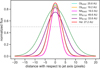 |
Fig. 9 Line-width profile of the emission lines analyzed in DL Tau. Each line profile is the result of a compilation of the Gaussian fits to intensity slices across the outflow/jet and their maximum intensity peaks are centered at the jet axis. The width of the outflow/jet, in au, is shown in the legend box. |
Jet wiggles as a potential sign of precession
The outflows/jets show different morphologies. When plotting the Gaussian centers in Fig. 3, it seems that in jets that are not too collimated, the amplitude of the wiggles is higher and asymmetric. As the wiggles do not show any clear periodic pattern, these are not associated with any inner disk misalignment. Instead, these are distinctive to the jet launching and evolution mechanism. Investigating whether there are any photometric variations in the inner disk of these sources could help us better understand whether there might be a body orbiting close to the central star (Petrov et al. 2001; Cody & Hillenbrand 2018). Fully 3D simulations of a MHD jet launching in young binaries, considering tidal forces (Sheikhnezami & Fendt 2015, 2018), have found that the inner disks will be warped and that the jet axis, which remains perpendicular to the disk, is subsequently re-aligned as a consequence of the disk precession.
The angle of the jet precession cone derived is slight and about 8°, but it could be much less – that is, perhaps approaching the differences between position angles identified here for T Tauri systems. However, their simulation was run only for one binary orbit and thus could not follow a whole precession period. Similar simulations, run in hydrodynamics but with forced precession of the jet nozzle, were applied for the precession jet source SS 433 (Monceau-Baroux et al. 2014), for example. These simulations show that the expected sinusoidal pattern of jet propagation varies along the jet, with larger amplitude and wavelength for more considerable distances, similar to our data indicating a jet cone opening up with distance. Furthermore, a more complex model fitting may be necessary to derive a conclusive statement about precession.
As we do not know the magnetic field structure and strength, defining a statement about the viability of kink modes in jets is not feasible. As an alternative to a precession of the jet axis, we might assume that the jet kink instability could cause the wiggling jet structure. Depending on the jet magnetization, this instability limits the expansion of the jet (Moll et al. 2008).
5 Conclusion
We analyzed spatially resolved emission lines, [O I] λλ6300, 6363, [N II] λλ6548, 6583, Hα, and [S II] λλ6716, 6730, in five T Tauris: DL Tau, CI Tau, DS Tau, IP Tau, and IM Lup hosting outflows/jets. We conducted an analysis to estimate the PAoutflow/jet of the emission lines coming from the innermost region of the disk. The average of the position angles for different emission lines was used to compare with the PAdust from the outer disk obtained in a previous work. We also performed a simple kinematic analysis to describe the velocity components of the line profiles and the line width of the outflow/jet in DL Tau. Finally, we calculated the mass-loss rate of the outflow/jet by using the [O I] λ6300 line based on physical parameters derived in this work. Our main conclusions are summarized as follows:
The PAoutflow/jet values are in good agreement, with differences of about 1°, except for IM Lup that is 2.1°, with the previously determined PAdust. Therefore, we do not find any evidence for a potential misalignment of the inner disk with regard to the outer disk.
The DL Tau and CI Tau emission lines are strongly blue-shifted, showing a velocity profile greater than 200 km s−1 associated with strong outflows/jets. The IP Tau, DS Tau, and IM Lup emission lines are less shifted and closely probing low-velocity components more associated with outflows and winds. The velocity components exhibit different outflows/jets and wind morphology in their systems.
The line width of the emission lines in DL Tau probes different layers in the outflow/jet, with the [O I] λ6363 line and the [N II] λ6583 line probing the deepest layer and the [S II] λ6716 line and the [S II] λ6730 line probing the widest layer. The [O I] λ6363 and [N II] λ6583 lines have very similar widths as well as Hα and [O I] λ6363 lines hinting to certain correlation in the ionization fraction and electronic density functions as mentioned in Lavalley-Fouquet et al. (2000).
Our estimated values for the mass loss are in agreement as being on the order of (1.1–6.5)×10−7–10−8 M⊙ yr−1, including the measurement of the length of the outflow/jet. This value is comparable to previous works for other sources and instruments.
Acknowledgements
We would like to thank the referee for providing useful comments in order to improve the quality and understanding of this work. This work is supported by the European Research Council (ERC) project under the European Union’s Horizon 2020 research and innovation programme number 757957. Thanks to Paola Pinilla for providing the dust continuum data. Also, thanks to Matthias Samland and Sebastiaan Haffert for useful discussions about the MUSE instrument and data analysis. This paper make use of the ALMA data: ADS/JAO.ALMA#2016.1.01164.S,ADS/JAO.ALMA#2016.1.00484.L, ADS/JAO.ALMA#2015.1.00888.S,ADS/JAO.ALMA#2017.A.00006.S. ALMA is a partnership of ESO (representing its member states), NSF (USA) and NINS (Japan), together with NRC (Canada), MOST and ASIAA (Taiwan), and KASI (Republic of Korea), in cooperation with the Republic of Chile. The Joint ALMA Observatory is operated by ESO, AUI/NRAO and NAOJ. N.K. acknowledges support provided by the Alexander von Humboldt Foundation in the framework of the Sofja Kovalevskaja Award endowed by the Federal Ministry of Education and Research. Th.H. acknowledges support from the European Research Council under the Horizon 2020 Framework Program via the ERC Advanced Grat Origins 83 24 28. G.-D.M. acknowledges the support of the DFG priority program SPP 1992 “Exploring the Diversity of Extrasolar Planets” (KU 2849/7-1 and MA 9185/1-1). G.-D.M. also acknowledges the support from the Swiss National Science Foundation under grant BSSGI0_155816 “PlanetsInTime”. Parts of this work have been carried out within the framework of the NCCR PlanetS supported by the Swiss National Science Foundation. S.K. acknowledges funding from UKRI in the form of a Future Leaders Fellowship (grant no. MR/T022868/1). We would like to thank the matplotlib team (Hunter 2007) for the good quality tool in order to better visualize the data. To Piqueras et al. (2017) for the mpdaf software to analyze the MUSE data.
Appendix A Example of linear model function
Figure A.1 shows an example of the linear function model for [O I] λ6300 in DL Tau to estimate the PAoutflow/jet. As mentioned in Sect. 3.1, we performed a Gaussian fit to maximum jet intensity peaks locations in each row in order to avoid any bias by noise in the data. These Gaussian centers are orthogonal with respect to the line model function in light blue. We applied the same methodology to the other sources in our sample. Figure A.2 shows the comparison between the maximum intensity peaks across the outflow/jet in blue and the intensity peaks fitted by a Gaussian in red.
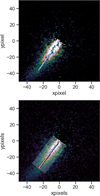 |
Fig. A.1 DL Tau [O I] λ6300 outflow/jet as an example of the linear model function (light blue) based on the Gaussian centers (grey dots, top). We fit 100 crossing lines (bottom) in order to estimate the width across the outflow/jet. |
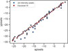 |
Fig. A.2 [O I] λ6300 successive outflow/jet intensity peaks across the jet axis in blue. We overplot the Gaussian centers from the fit in red, which is then used to estimate the PAoutflow/jet. The deviations of the outflow/jet intensity peaks could be caused by noise in the data. |
Appendix B Outflow/jet lengths
To determine the length of the outflow/jet, the linear model function goes across the outflow/jet until it reaches the rms of the image. The number of elements or pixels representing the length are in Table B.1. The starting point of the outflow/jet length comes from the center of the image, where the star is located. We consider these lengths when calculating the mass-loss rate using the [O I] λ6300 in §3.4.
Outflow/jet length estimates.
Appendix C Disk inclination and rotation
In Figure C.2, we identify whether these disk-outflow (disk-jet) systems have positive or negative inclination to determine the direction to where the disk is rotating. We look at the rotation of the system based on the 12CO channel maps. For IM Lup, we use Pinte et al. (2020). Also, the inclination of IM Lup can easily be seen by looking at the bright side of the disk in near-infrared image from Avenhaus et al. (2018). For CI Tau, we use Rosotti et al. (2021). For IP Tau and DS Tau, we use Simon et al. (2017). For DL Tau, there is no evidence of the 12CO channel maps in the literature nor any observations taken and posted in the ALMA archive. By looking at the blue-shifted outflow/jet in the MUSE image, it is intuitive that we are looking at the back side of the disk in DL Tau. For PDS 70, we use Keppler et al. (2019) and Isella et al. (2019).
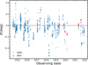 |
Fig. C.1 Residual rotation of the WFM observations (blue) taken until late 2021 and the NFM observations (red). Note: the NFM residuals are less than 0.2 degrees. |
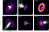 |
Fig. C.2 Composite images of disk-outflow (disk-jet) systems. The outflows/jets are superimposed to the dust continuum disk detected by ALMA Cycle 4 at 1.33 mm (Long et al. 2018). The arrows, representing the redshifted and blueshifted velocity components, shows the disk rotation. With this determination, IM Lup, DS Tau, PDS 70 (the top three panels) as well as DL Tau and IP Tau have a negative disk inclination, whereas, CI Tau have a positive inclination. The outflow/jet in CI Tau, IP tau, and DL Tau is comprised of the emission from [O I] λ6300. For IM Lup, and DS Tau are [N II] λ6583. Lastly, we decided to try out the data set of PDS 70 already published by Haffert et al. (2019), as there is some emission at the center seen in Hα. The disk inclination is −51.7±0.1 and the PAdust is 156.7±0.1° as derived from ALMA Cycle 5 continuum observations at 0.855 mm by (see also Isella et al. 2019; Keppler et al. 2019). We estimated the PAoutflow/jet for PDS 70 as 154.82±5.92°. |
Appendix D Rotational offset analysis in MUSE
We carried out a residual rotation analysis for the NFM data of globular clusters in order to obtain the accuracy of the MUSE field-of-view orientation (see Kamann et al. (2018)). This analysis was done with PAMPELMUSE software (Kamann et al. 2013), which uses the centers of dense star clusters, which have been pre-imaged with Hubble Space Telescope (HST) – and then the stars available are identified in the astrometric reference catalogues in the MUSE cubes. This is done using a coordinate transformation with six parameters that takes into account shifts along the x- and y-axes, while other parameters are measure of distortions and rotations. Figure C.1 shows the residual rotation for all the wide-field mode (WFM) observations (blue) taken until late 2021 and the NFM observations (red). From the first sight, there is no systematic difference between the results derived from WFM and NFM cubes, which is reassuring and the resulting uncertainty is less than 1 degree for both modes – and less than 0.2 degrees for the NFM in particular. The same analysis was used by Emsellem et al. (2022), where the MUSE field of view orientation is of the order of a few tenths of a degree. Based on this residual analysis, we consider the rotational accuracy of MUSE NFM to be 0.2 degrees, which is a conservative selection (see column 8 in Table 2). As expected, this uncertainty value does not change the actual uncertainty estimates for our PAoutflow/jet reported in Table 2.
Appendix E Spectrum
Figure E.1, Figure E.2, and Figure E.3 show the spectrum by spatially summing the area enclosed to the jet over all channels for all sources presented in this work. In the upper-right, we zoom onto the wavelength range where the seven forbidden emission lines are identified and analyzed here. DL Tau shows the best signal-to-noise emission in all of the seven lines analyzed here. The DL Tau spectrum shows the presence of just a couple of more emission lines in the blue regime, such as Hβ λ4861 as well as a weak one at ~5156 Å (see Fig. E.1a). We also found very faint emission of Hβ in DS Tau and CI Tau. We report emission lines in the red optical regime as well at around [Ca II] λ7288, [O II] λλ7320, 7329, 7373, and [Fe II] λλ 8619, 8892 for DL Tau and CI Tau, which host strong outflows/jets. We encourage further analysis of these other lines that lie out of the scope of this paper. The strong outflow/jet is seen very clear and collimated in all seven emission lines in DL Tau, reaching close to 200 au in extension. As a comparison, the extension of the outflow/jet in CI Tau only reach around 60 au.
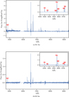 |
Fig. E.1 Spectrum in the area enclosed to the jets of DL Tau and DS Tau. |
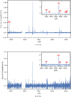 |
Fig. E.2 Spectrum in the area enclosed to the jets of CI Tau and IP Tau. |
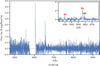 |
Fig. E.3 Spectrum in the area enclosed to the jet of IM Lup. |
Appendix F Resolution profile
Table F.1 shows the summary of the spectral resolution properties to be compared to the line-broadening of MUSE (see Figure 8). Figure F.1, Figure F.2, Figure F.3, Figure F.4, and Figure F.5 show the actual line profile for all five disk-outflow/jet systems. We note that most of the lines analyzed here are marginally resolved, meaning the observed line width (red curve) is very close to the line-broadening of MUSE (black-dashed line).
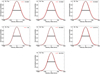 |
Fig. F.1 DL Tau line widths in red compared to the line-broadening of MUSE in black-dashed line. |
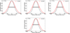 |
Fig. F.2 CI Tau line widths in red compared to the line-broadening of MUSE in black-dashed line. |
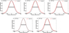 |
Fig. F.3 DS Tau line widths in red compared to the line-broadening of MUSE in black-dashed line. |
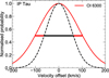 |
Fig. F.4 IP Tau line widths in red compared to the line-broadening of MUSE in black-dashed line. |
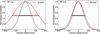 |
Fig. F.5 IM Lup line widths in red compared to the line-broadening of MUSE in black-dashed line. |
References
- Andrews, S. M., Huang, J., Pérez, L. M., et al. 2018, ApJ, 869, L41 [NASA ADS] [CrossRef] [Google Scholar]
- Antoniucci, S., García López, R., Nisini, B., et al. 2011, A&A, 534, A32 [NASA ADS] [CrossRef] [EDP Sciences] [Google Scholar]
- Avenhaus, H., Quanz, S. P., Garufi, A., et al. 2018, ApJ, 863, 44 [NASA ADS] [CrossRef] [Google Scholar]
- Bacciotti, F., Mundt, R., Ray, T. P., et al. 2000, ApJ, 537, L49 [NASA ADS] [CrossRef] [Google Scholar]
- Bacon, R., Accardo, M., Adjali, L., et al. 2010, SPIE Conf. Ser., 7735, 773508 [Google Scholar]
- Bai, X.-N., & Stone, J. M. 2013, ApJ, 769, 76 [Google Scholar]
- Balbus, S. A., & Hawley, J. F. 1991, ApJ, 376, 214 [Google Scholar]
- Banzatti, A., Pascucci, I., Edwards, S., et al. 2019, ApJ, 870, 76 [Google Scholar]
- Benisty, M., Stolker, T., Pohl, A., et al. 2017, A&A, 597, A42 [NASA ADS] [CrossRef] [EDP Sciences] [Google Scholar]
- Benisty, M., Juhász, A., Facchini, S., et al. 2018, A&A, 619, A171 [NASA ADS] [CrossRef] [EDP Sciences] [Google Scholar]
- Blandford, R. D., & Payne, D. G. 1982, MNRAS, 199, 883 [CrossRef] [Google Scholar]
- Bohn, A. J., Benisty, M., Perraut, K., et al. 2022, A&A, 658, A183 [NASA ADS] [CrossRef] [EDP Sciences] [Google Scholar]
- Brown, P. J., Fuller, W. A., et al. 1990, Statistical analysis of measurement error models and applications, Proceedings of the AMS-IMS-SIAM joint summer research conference held June 10-16, 1989, with support from the National Science Foundation and the US Army Research Office, 112 (American Mathematical Society) [Google Scholar]
- Casassus, S., Avenhaus, H., Pérez, S., et al. 2018, MNRAS, 477, 5104 [NASA ADS] [CrossRef] [Google Scholar]
- Casse, F., & Ferreira, J. 2000, A&A, 353, 1115 [NASA ADS] [Google Scholar]
- Casse, F., & Keppens, R. 2002, ApJ, 581, 988 [Google Scholar]
- Cody, A. M., & Hillenbrand, L. A. 2018, AJ, 156, 71 [Google Scholar]
- Debes, J. H., Poteet, C. A., Jang-Condell, H., et al. 2017, ApJ, 835, 205 [NASA ADS] [CrossRef] [Google Scholar]
- Donati, J. F., Bouvier, J., Alencar, S. H., et al. 2019, MNRAS, 483, L1 [Google Scholar]
- Dougados, C., Cabrit, S., Lavalley, C., & Ménard, F. 2000, A&A, 357, L61 [NASA ADS] [Google Scholar]
- Edwards, S., Cabrit, S., Strom, S. E., et al. 1987, ApJ, 321, 473 [Google Scholar]
- Ellerbroek, L. E., Podio, L., Dougados, C., et al. 2014, A&A, 563, A87 [NASA ADS] [CrossRef] [EDP Sciences] [Google Scholar]
- Emsellem, E., Schinnerer, E., Santoro, F., et al. 2022, A&A, 659, A191 [NASA ADS] [CrossRef] [EDP Sciences] [Google Scholar]
- Ercolano, B., & Pascucci, I. 2017, Roy. Soc. Open Sci., 4, 170114 [Google Scholar]
- Eriksson, S. C., Asensio Torres, R., Janson, M., et al. 2020, A&A, 638, A6 [Google Scholar]
- Fang, M., Pascucci, I., Edwards, S., et al. 2018, ApJ, 868, 28 [NASA ADS] [CrossRef] [Google Scholar]
- Fendt, C., & Zinnecker, H. 1998, A&A, 334, 750 [NASA ADS] [Google Scholar]
- Gaia Collaboration (Brown, A. G. A., et al.) 2021, A&A, 649, A1 [NASA ADS] [CrossRef] [EDP Sciences] [Google Scholar]
- Giannini, T., Antoniucci, S., Nisini, B., Bacciotti, F., & Podio, L. 2015, ApJ, 814, 52 [NASA ADS] [CrossRef] [Google Scholar]
- GRAVITY Collaboration (Bouarour, Y. I., et al.) 2020, A&A, 642, A162 [NASA ADS] [CrossRef] [EDP Sciences] [Google Scholar]
- Haffert, S. Y., Bohn, A. J., de Boer, J., et al. 2019, Nat. Astron., 3, 749 [Google Scholar]
- Hamann, F. 1994, ApJS, 93, 485 [NASA ADS] [CrossRef] [Google Scholar]
- Hartigan, P., Morse, J. A., & Raymond, J. 1994, ApJ, 436, 125 [NASA ADS] [CrossRef] [Google Scholar]
- Hartigan, P., Edwards, S., & Ghandour, L. 1995, ApJ, 452, 736 [Google Scholar]
- Hashimoto, J., Aoyama, Y., Konishi, M., et al. 2020, AJ, 159, 222 [Google Scholar]
- Hirth, G. A., Mundt, R., & Solf, J. 1997, A&As, 126, 437 [NASA ADS] [CrossRef] [EDP Sciences] [Google Scholar]
- Huang, J., Andrews, S. M., Dullemond, C. P., et al. 2018, ApJ, 869, L42 [NASA ADS] [CrossRef] [Google Scholar]
- Hunter, J. D. 2007, Comput. Sci. Eng., 9, 90 [NASA ADS] [CrossRef] [Google Scholar]
- Isella, A., Benisty, M., Teague, R., et al. 2019, ApJ, 879, L25 [Google Scholar]
- Kamann, S., Wisotzki, L., & Roth, M. M. 2013, A&A, 549, A71 [NASA ADS] [CrossRef] [EDP Sciences] [Google Scholar]
- Kamann, S., Husser, T. O., Dreizler, S., et al. 2018, MNRAS, 473, 5591 [NASA ADS] [CrossRef] [Google Scholar]
- Keppler, M., Teague, R., Bae, J., et al. 2019, A&A, 625, A118 [NASA ADS] [CrossRef] [EDP Sciences] [Google Scholar]
- Lavalley-Fouquet, C., Cabrit, S., & Dougados, C. 2000, A&A, 356, L41 [NASA ADS] [Google Scholar]
- Long, F., Pinilla, P., Herczeg, G. J., et al. 2018, ApJ, 869, 17 [Google Scholar]
- Long, F., Herczeg, G. J., Harsono, D., et al. 2019, ApJ, 882, 49 [Google Scholar]
- Marino, S., Perez, S., & Casassus, S. 2015, ApJ, 798, L44 [Google Scholar]
- Marleau, G. D., Aoyama, Y., Kuiper, R., et al. 2022, A&A, 657, A38 [NASA ADS] [CrossRef] [EDP Sciences] [Google Scholar]
- Min, M., Stolker, T., Dominik, C., & Benisty, M. 2017, A&A, 604, A10 [Google Scholar]
- Moll, R., Spruit, H. C., & Obergaulinger, M. 2008, A&A, 492, 621 [NASA ADS] [CrossRef] [EDP Sciences] [Google Scholar]
- Monceau-Baroux, R., Porth, O., Meliani, Z., & Keppens, R. 2014, A&A, 561, A30 [NASA ADS] [CrossRef] [EDP Sciences] [Google Scholar]
- Muro-Arena, G. A., Benisty, M., Ginski, C., et al. 2020, A&A, 635, A121 [NASA ADS] [CrossRef] [EDP Sciences] [Google Scholar]
- Natta, A., Testi, L., Alcalá, J. M., et al. 2014, A&A, 569, A5 [NASA ADS] [CrossRef] [EDP Sciences] [Google Scholar]
- Nisini, B., Antoniucci, S., Alcalá, J. M., et al. 2018, A&A, 609, A87 [EDP Sciences] [Google Scholar]
- Pascucci, I., Banzatti, A., Gorti, U., et al. 2020, ApJ, 903, 78 [Google Scholar]
- Petrov, P. P., Pelt, J., & Tuominen, I. 2001, A&A, 375, 977 [NASA ADS] [CrossRef] [EDP Sciences] [Google Scholar]
- Piétu, V., Dutrey, A., & Guilloteau, S. 2007, A&A, 467, 163 [Google Scholar]
- Pinilla, P., Benisty, M., Cazzoletti, P., et al. 2019, ApJ, 878, 16 [Google Scholar]
- Pinte, C., Price, D. J., Ménard, F., et al. 2020, ApJ, 890, L9 [CrossRef] [Google Scholar]
- Piqueras, L., Conseil, S., Shepherd, M., et al. 2017, arXiv e-prints, [arXiv:1710.03554] [Google Scholar]
- Podio, L., Bacciotti, F., Nisini, B., et al. 2006, A&A, 456, 189 [NASA ADS] [CrossRef] [EDP Sciences] [Google Scholar]
- Proxauf, B., Öttl, S., & Kimeswenger, S. 2014, A&A, 561, A10 [NASA ADS] [CrossRef] [EDP Sciences] [Google Scholar]
- Rigliaco, E., Pascucci, I., Gorti, U., Edwards, S., & Hollenbach, D. 2013, ApJ, 772, 60 [NASA ADS] [CrossRef] [Google Scholar]
- Rodenkirch, P. J., Klahr, H., Fendt, C., & Dullemond, C. P. 2020, A&A, 633, A21 [NASA ADS] [CrossRef] [EDP Sciences] [Google Scholar]
- Rosotti, G. P., Ilee, J. D., Facchini, S., et al. 2021, MNRAS, 501, 3427 [Google Scholar]
- Sheikhnezami, S., & Fendt, C. 2015, ApJ, 814, 113 [NASA ADS] [CrossRef] [Google Scholar]
- Sheikhnezami, S., & Fendt, C. 2018, ApJ, 861, 11 [NASA ADS] [CrossRef] [Google Scholar]
- Sheikhnezami, S., Fendt, C., Porth, O., Vaidya, B., & Ghanbari, J. 2012, ApJ, 757, 65 [NASA ADS] [CrossRef] [Google Scholar]
- Simon, M. N., Pascucci, I., Edwards, S., et al. 2016, ApJ, 831, 169 [Google Scholar]
- Simon, M., Guilloteau, S., Di Folco, E., et al. 2017, ApJ, 844, 158 [Google Scholar]
- Solf, J., & Boehm, K. H. 1993, ApJ, 410, L31 [NASA ADS] [CrossRef] [Google Scholar]
- Soummer, R., Pueyo, L., & Larkin, J. 2012, ApJ, 755, L28 [Google Scholar]
- Stepanovs, D., & Fendt, C. 2016, ApJ, 825, 14 [Google Scholar]
- Stolker, T., Dominik, C., Avenhaus, H., et al. 2016, A&A, 595, A113 [NASA ADS] [CrossRef] [EDP Sciences] [Google Scholar]
- Weilbacher, P. M., Streicher, O., Urrutia, T., et al. 2012, SPIE Conf. Ser., 84510B [Google Scholar]
- Weilbacher, P. M., Streicher, O., Urrutia, T., et al. 2014, in ASP, Conf. Ser., 485, 451 [NASA ADS] [Google Scholar]
- Weilbacher, P. M., Streicher, O., & Palsa, R. 2016, MUSE-DRP: MUSE Data Reduction Pipeline [Google Scholar]
- Weilbacher, P. M., Palsa, R., Streicher, O., et al. 2020, A&A, 641, A28 [NASA ADS] [CrossRef] [EDP Sciences] [Google Scholar]
- Whelan, E. T., Pascucci, I., Gorti, U., et al. 2021, ApJ, 913, 43 [NASA ADS] [CrossRef] [Google Scholar]
- Woitas, J., Ray, T. P., Bacciotti, F., Davis, C. J., & Eislöffel, J. 2002, ApJ, 580, 336 [NASA ADS] [CrossRef] [Google Scholar]
- Xie, C., Haffert, S. Y., de Boer, J., et al. 2020, A&A, 644, A149 [EDP Sciences] [Google Scholar]
All Tables
All Figures
|
Fig. 1 Composite image of different protoplanetary disks at four different forbidden emission lines. First column shows the dust continuum emission at 1.3 mm from ALMA cycle 4 (Long et al. 2018, 2019). Other columns show the different forbidden emission lines from MUSE as labeled in the top left of the first row. Dashed yellow rectangles mark the area from where we gather the spectrum of the jet by summing over the spatial axes within the dashed yellow frame of the image. |
| In the text | |
|
Fig. 2 Visualization of the estimated |
| In the text | |
|
Fig. 3 Successive Gaussian centers shown as navy-colored dots. Wiggles are seen in DL Tau and IP Tau at [O I] λ6300, and for CI Tau, DS Tau, and IM Lup at [N II] λ6583. |
| In the text | |
|
Fig. 4 Hα line profile identified for DL Tau probing the high line-of-sight velocity component coming from the strong outflow/jet. The red dashed line represent the line-of-sight maximum velocity. |
| In the text | |
|
Fig. 5 [O I] λ6300 line proflies identified in five sources from our sample. DL Tau and CI Tau have their line centered at velocities greater than 100 km s−1, which is characteristic of jets. Unlike DL Tau and CI Tau, the disks of DS Tau, IP Tau, and IM Lup show smaller shifts of less than 100 km s−1 and broader line widths significantly overlapping with 0 km s−1, possibly including the LVC emission as a result. DS Tau has the most centered line. |
| In the text | |
|
Fig. 6 [N II]/λ6583 line profiles identified in four sources from our sample. Same case as in Fig. 5, DL Tau and CI Tau probe high-velocity components, while DS Tau and IM Lup are more centered to zero. |
| In the text | |
|
Fig. 7 [SII] λ6730 line profile identified for DL Tau, CI Tau, and DS Tau. |
| In the text | |
|
Fig. 8 Spectral resolution, R = λ/Δλ, versus wavelength of the seven forbidden emission lines used in the analysis here. The blue curve shows the resolution curve of MUSE at increments of 500 Å. Each R value for each line is linearly interpolated from the MUSE resolution curve. The values were obtained from the MUSE User Manual (version 11.4, Fig. 18). |
| In the text | |
|
Fig. 9 Line-width profile of the emission lines analyzed in DL Tau. Each line profile is the result of a compilation of the Gaussian fits to intensity slices across the outflow/jet and their maximum intensity peaks are centered at the jet axis. The width of the outflow/jet, in au, is shown in the legend box. |
| In the text | |
|
Fig. A.1 DL Tau [O I] λ6300 outflow/jet as an example of the linear model function (light blue) based on the Gaussian centers (grey dots, top). We fit 100 crossing lines (bottom) in order to estimate the width across the outflow/jet. |
| In the text | |
|
Fig. A.2 [O I] λ6300 successive outflow/jet intensity peaks across the jet axis in blue. We overplot the Gaussian centers from the fit in red, which is then used to estimate the PAoutflow/jet. The deviations of the outflow/jet intensity peaks could be caused by noise in the data. |
| In the text | |
|
Fig. C.1 Residual rotation of the WFM observations (blue) taken until late 2021 and the NFM observations (red). Note: the NFM residuals are less than 0.2 degrees. |
| In the text | |
|
Fig. C.2 Composite images of disk-outflow (disk-jet) systems. The outflows/jets are superimposed to the dust continuum disk detected by ALMA Cycle 4 at 1.33 mm (Long et al. 2018). The arrows, representing the redshifted and blueshifted velocity components, shows the disk rotation. With this determination, IM Lup, DS Tau, PDS 70 (the top three panels) as well as DL Tau and IP Tau have a negative disk inclination, whereas, CI Tau have a positive inclination. The outflow/jet in CI Tau, IP tau, and DL Tau is comprised of the emission from [O I] λ6300. For IM Lup, and DS Tau are [N II] λ6583. Lastly, we decided to try out the data set of PDS 70 already published by Haffert et al. (2019), as there is some emission at the center seen in Hα. The disk inclination is −51.7±0.1 and the PAdust is 156.7±0.1° as derived from ALMA Cycle 5 continuum observations at 0.855 mm by (see also Isella et al. 2019; Keppler et al. 2019). We estimated the PAoutflow/jet for PDS 70 as 154.82±5.92°. |
| In the text | |
|
Fig. E.1 Spectrum in the area enclosed to the jets of DL Tau and DS Tau. |
| In the text | |
|
Fig. E.2 Spectrum in the area enclosed to the jets of CI Tau and IP Tau. |
| In the text | |
|
Fig. E.3 Spectrum in the area enclosed to the jet of IM Lup. |
| In the text | |
|
Fig. F.1 DL Tau line widths in red compared to the line-broadening of MUSE in black-dashed line. |
| In the text | |
|
Fig. F.2 CI Tau line widths in red compared to the line-broadening of MUSE in black-dashed line. |
| In the text | |
|
Fig. F.3 DS Tau line widths in red compared to the line-broadening of MUSE in black-dashed line. |
| In the text | |
|
Fig. F.4 IP Tau line widths in red compared to the line-broadening of MUSE in black-dashed line. |
| In the text | |
|
Fig. F.5 IM Lup line widths in red compared to the line-broadening of MUSE in black-dashed line. |
| In the text | |
Current usage metrics show cumulative count of Article Views (full-text article views including HTML views, PDF and ePub downloads, according to the available data) and Abstracts Views on Vision4Press platform.
Data correspond to usage on the plateform after 2015. The current usage metrics is available 48-96 hours after online publication and is updated daily on week days.
Initial download of the metrics may take a while.