| Issue |
A&A
Volume 669, January 2023
|
|
|---|---|---|
| Article Number | A9 | |
| Number of page(s) | 18 | |
| Section | Stellar atmospheres | |
| DOI | https://doi.org/10.1051/0004-6361/202244924 | |
| Published online | 23 December 2022 | |
Chromospheric activity and photospheric variation of α Ori during the great dimming event in 2020
1
Hamburger Sternwarte, Universität Hamburg,
Gojenbergsweg 112,
21029
Hamburg, Germany
e-mail: This email address is being protected from spambots. You need JavaScript enabled to view it.
2
Departamento de Astronomía, Universidad de Guanajuato,
Callejön de Jalisco s/n,
36023
Guanajuato, GTO, Mexico
3
Kimmel fellow, Department of Earth and Planetary Science, Weizmann Institute of Science,
Herzl St 234,
Rehovot, Israel
Received:
8
September
2022
Accepted:
1
October
2022
Abstract
Aims. The so-called great dimming event of α Ori in late 2019 and early 2020 sparked our interest in the behaviour of chromospheric activity during this period. α Ori was already part of the long-term monitoring program of our TIGRE telescope to study the stellar activity of giant stars, and therefore regular measurements of α Ori have been taken since 2013.
Methods. In the context of this study, we determined the TIGRE S -index values and, using a set of calibration stars, converted these to the Mount Wilson S -index scale, which allows us to combine our TIGRE activity measurements with the SMWO values taken during the landmark Mount Wilson program some decades earlier and to compare that extended time series with the visual and V magnitude photometric data from the AAVSO database. In addition, we determined the absolute and normalised excess flux of the Ca II H&K lines. To understand the activity in absolute terms, we also assessed the changes in effective temperature using the TiO bands covered by our TIGRE spectra.
Results. We find a clear drop in effective temperature by about 80 K between November 2019 and February 2020, which coincides with the minimum of visual brightness. In addition, the effective (luminous) photospheric area of α Ori also shrank. This might be related to a temporary synchronisation of several large convective cells in cooling and sinking down. During the same period, the S-index increased significantly, yet this is a mere contrast effect, because the normalised excess flux of the Ca II H&K lines did not change significantly. However, the latter dropped immediately after this episode. Comparing the combined SMWO values and visual magnitude time series, we find a similar increase in the S -index during another noticeable decrease in the visual magnitude of α Ori which took place in 1984 and 1985. These two episodes of dimming therefore seem to share a common nature. To probe the dynamics of the upper photosphere, we further analysed the closely neighbouring lines of V I and Fe I at 6251.82 and 6251.56 Å respectively. Remarkably, their core distance varies, and once converted to radial velocity, shows a relation with the great dimming event, as well as with the consecutive, weaker dimming episode in the observing season of 2020 and 2021. This type of variation could be caused by rising and sinking cool plumes as a temporary spill-over of convection on α Ori.
Conclusions. As the effective temperature of α Ori is variable, the S -index, computed relative to a near-ultraviolet (NUV) continuum, is only of restricted use for any monitoring study of the chromospheric activity of α Ori. It is therefore important to consider the effective temperature variability and derive the normalised Ca II H&K flux to study the chromospheric long-term changes in absolute terms. In fact, the Ca II H&K normalised excess flux time series shows that the chromospheric emission of α Ori did not change significantly between November 2019 and February 2020, but then beyond the great dimming minimum it does vary. Hence, this delay of the chromospheric reaction suggests that the cause for the great dimming is located in the photosphere. An investigation of the long-term spectroscopic and photometric time series of α Ori suggests that the great dimming in 2019 and 2020 does not appear to be a unique phenomenon, but rather that such dimmings do occur more frequently, which motivates further monitoring of α Ori with facilities such as TIGRE.
Key words: stars: activity / stars: chromospheres / supergiants
© The Authors 2022
 Open Access article, published by EDP Sciences, under the terms of the Creative Commons Attribution License (https://creativecommons.org/licenses/by/4.0), which permits unrestricted use, distribution, and reproduction in any medium, provided the original work is properly cited.
This article is published in open access under the Subscribe-to-Open model. This email address is being protected from spambots. You need JavaScript enabled to view it. to support open access publication.
1 Introduction
The red supergiant α Ori (HD 39801, Betelgeuse) is one of the brightest stars in the sky and showed an unusual decrease in its brightness in the winter between 2019 and 2020. Normally, the brightness of α Ori typically varies between ~0.2 mag and ~1 mag in the Johnson V-band, as demonstrated by a light curve available in the AAVSO (American Association of Variable Star Observers) database1. However, in February 2020, the brightness of a Ori decreased extraordinarily to a mere V ~ 1.6 mag, an event that was consequently dubbed the ‘great dimming event’. In December 2019, Guinan et al. (2019) raised public awareness of this event, and an ESO press release2 showed VLT/SPHERE (Very Large Telescope/Spectro-Polarimetric High-contrast Exoplanet REsearch instrument) observations of α Ori by Montargès, comparing its state in January 2019 with that in December 2019; this VLT/SPHERE image confirmed the significant darkening of Betelgeuse in comparison to an image taken in January 2019.
As to the cause of the unusual decrease in brightness, two main hypotheses were put forward: the first interprets the cause of the dimming to be a decrease in effective temperature, that is, a photospheric effect, while the alternative hypothesis argues that the photospheric emission had been shielded by material from some ejection or increased mass-loss event, thus located further out and not directly related to the photosphere.
Levesque & Massey (2020) studied low-resolution spectra of α Ori; while finding a small drop in effective temperature, the authors argue that this decrease is too small to explain the great dimming and suggest instead a mass ejection as an explanation for the observed decrease in brightness. This scenario is supported by Dupree et al. (2020), who analysed the mid-ultraviolet (MUV) flux in 2400-2700 Å and Mg II h&k lines with spectra taken with HST/STIS (Hubble Space Telescope/Space Telescope Imaging Spectrograph), and found that both fluxes, as measured in September 2019, October 2019, and November 2019, were larger than in February 2020 at the maximum of the great dimming event. Therefore, Dupree et al. (2020) argue that a great mass ejection occurred in October 2019 leading to the formation of a dust cloud in the following weeks, which eventually darkened a Ori. Dust dimming of a Ori is also supported by the work of Montargès et al. (2021), who analysed VLT/SPHERE images taken in January 2019, December 2019, January 2020, and March 2020.
On the other hand, the dust cloud theory was disputed by Dharmawardena et al. (2020), who investigated submillimetre (submm) data taken with the James Clerk Maxwell Telescope and Atacama Pathfinder Experiment. While Dharmawardena et al. (2020) also found α Ori to be about 20% fainter in the submm range, their radiative modelling suggests that the dimming event was caused by some photospheric change. More specifically, a change in effective temperature during the great dimming was also demonstrated by Harper et al. (2020), who present a TiO band light curve; based on these observations, the derived effective temperature time series shows a significant drop, which coincides well with the great dimming event as observed in the V-band.
In this paper we present our α Ori observations obtained with the 1.2 m TIGRE telescope (for more details, see Schmitt et al. 2014; González-Pérez et al. 2022; and below), an instrument designed primarily for the study of stellar chromospheric activity. However, before we present our respective results in more detail, we need to address the changes in effective temperature, because these imply physical changes of the photosphere leading to changes in the spectral fluxes, which are used as a reference in many activity indicators. Consequently, the drop in temperature around February 2020 has a direct impact on the interpretation of the observed activity indicators, such as the calibrated Mount Wilson S -index, as well as the derivation of the absolute Ca II H&K line flux of α Ori. Thereafter, we present a combined time series of the Mount Wilson S -index and compare its behaviour to photometric data.
Furthermore, we derive the absolute and excess Ca II H&K line flux, which show a remarkably different relation with the V-band light curve. Also, we present the significant line depth and radial-velocity (RV) variations of the unequal neighbouring line pair of V I 6251.82 Å and Fe I 6252.56 Å. These lines form in different depths of the photosphere and are indicative of a height-dependent dynamical behaviour of the photosphere apparently associated with the great dimming event. Finally, we summarise our results and present our conclusion about the possible physical causes for this dimming event.
2 TIGRE spectroscopic monitoring and data reduction
TIGRE (Telescopio Internacional de Guanajuato Robótico Espectroscópico) is a fully robotic spectroscopic telescope with an aperture of 1.2 m, located at the La Luz Observatory of the University of Guanajuato, Mexico, designed for long term monitoring programs. The two-spectral-channel, fibre-fed Échelle spectrograph HEROS (Heidelberg Extended Range Optical Spectrograph) is located in a thermally and mechanically isolated room. The spectral resolving power of the HEROS spectrograph is R ≈ 20 000, which is relatively uniform over a wavelength range from 3800 Å to 8800 Å with a minor gap around 5800 Å between the two spectral channels caused by the dichroic beam splitter; the TIGRE facility and the realisation of its robotic operation is described in more detail by Schmitt et al. (2014) and González-Pérez et al. (2022).
The TIGRE/HEROS spectra used here were reduced with the TIGRE automatic standard reduction pipeline v3.1 written in IDL based on the reduction package REDUCE (Piskunov & Valenti 2002). This latter pipeline includes all required reduction steps for an Échelle spectrum; a detailed description of the first version of the TIGRE reduction pipeline is given by Mittag et al. (2010), and additional information can be found in Hempelmann et al. (2016) and Mittag et al. (2016).
The TIGRE observing plan includes a monitoring program of the chromospheric activity of giant stars, providing a study of the variations of the Ca II H&K lines. One target of this program is the red supergiant α Ori. Until November 2019, with the goal of studying long-term variability, α Ori was for the most part observed with a monthly cadence. However, in December 2019, we started covering α Ori more frequently to better monitor the stellar activity during the great dimming event. In Table 1, we list the number of observations taken in each observing season and the range of the signal-to-noise ratio (S/N) at 4000 Å per season.
α Ori observations by observing season (September-April).
3 Assessment of long-term effective temperature variations
Before discussing the chromospheric activity of α Ori, we try to quantify the possible variations of the effective temperature during the great dimming event in order to consider this in our quantitative analysis of the chromospheric activity at this point in time. To begin with, we used the publicly available photometric data from the AAVSO database as a reference to the timing of the great dimming event. Various colour indices provide an indicator of the effective temperature. However, since their variation could in principle be caused partly by extinction from dust, we also use TiO bands here to estimate the effective temperature from our TIGRE/HEROS spectra by comparing the TiO bands of each TIGRE/HEROS spectrum with best-matching PHOENIX atmospheric model spectra.
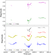 |
Fig. 1 Light curves of the B, V, R, I, J, and H bands, beginning with 2018.5. The upper panel depicts the J and H magnitudes, and the lower panel shows the B, V, R, and I bands. |
3.1 Time series of photometric data and colour indices
Starting with epoch 2018.5, in Fig. 1 we show the daily brightness in the B, V, R, I, J, and H bands, as listed in the AAVSO database. In all bands, the light curves show a variation apparently caused by a pulsation cycle, its amplitude being smaller in the J and H bands. Next, we computed the B − V, V − R, R − I, and J − H colour indices for every day with available data; to ensure that any variation is real, we only provide values with a relative error of lower than 5% of the respective index. These values are shown in Fig. 2, which demonstrates that variations occur in all four colour indices; the times and values of these changes are consistent with the effective temperature variation shown by Harper et al. (2020). The colour indices R − I and J − H increase during the great dimming event, which shows a minimum in the light curve in each band. Both indices show the behaviour expected, that is, a decrease in the effective temperature, which manifests as an increase in these two indices; see Appendix B. However, the colour index V − R shows strong scatter during the minimum of the light curves, without any clear trend, and the B − V colour index actually decreases during the great dimming event.
While over a large temperature range in cool stars the B − V index increases with decreasing effective temperature, this is not the case here − the coolest stars form an exception. In fact, B − V values calculated from PHOENIX spectra of an effective temperature of less than 3600 K show the same behaviour. Above 3600 K, with rising effective temperature, the B − V values also decrease from their maximum value there, but very slowly at first. The B − V values based on PHOENIX spectra (Husser et al. 2013) are shown in Fig. B.2 and further explanation of their derivation is given in Appendix B. This inverted B − V behaviour was also found in the super giant star HD 156014 (α Her A). This object has a B − V colour of only 1.164 mag (ESA 1997), but an effective temperature as low as 3271 K (taken from the PASTEL catalogue, Version 2020-01-30; Soubiran et al. 2016). Interestingly, a similar trend inversion was shown by Lançon et al. (2007) for the H − K index, calculated from PHOENIX spectra for red supergiants and giants.
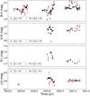 |
Fig. 2 Colour index time series. The top panel shows the B − V values, the second displays the V − R values, the third the R − I values, and the lowest panel depicts the H − J values. Black dots represent values with a relative error of lower than 2%, whereas red data points those lower than 5%. |
3.2 Effective temperature assessment based on TiO bands
To perform a quantitative assessment of any effective temperature variations, we now use the TiO bands; these bands become stronger in cooler stars and thereby provide a good effective temperature indicator in their own right. Examining the TiO band at 7054 Å, in Fig. 3 we compare four TIGRE spectra taken before, during, and after the great dimming event and indeed find a decrease in their normalised fluxes during the great dimming; this finding indicates that the effective temperature dropped during the great dimming event.
To quantify the effective temperature based on the TiO bands strength, we compared four normalised TiO bands at 4954 Å, 5450 Å, 6154 Å, and 7054 Å in the TIGRE spectra with normalised PHOENIX spectra of the Göttingen University database created by Husser et al. (2013), in a temperature range from 3300 Å to 3900 K (with a step size of 100 K, a log g of 0.0, and solar metallicity). For this comparison, the rotational line-broadening (v sin(i)) and a spectral resolving power of R ≈ 20000 are considered in the PHOENIX spectrum.
To estimate the differences between observed spectra and PHOENIX spectra, and to find the best matches, we computed the χ2 values of the residuals for this effective temperature range of the PHOENIX models. The effective temperatures determined in this way for each band and each TIGRE spectrum are shown in the upper panel of Fig. 4. Ideally, these different temperatures should agree, but systematic differences illustrate the remaining shortcomings of the models in extreme non-local thermodynamic equilibrium (non-LTE) conditions under very low gravity and in very extended and possibly non-spherically symmetric atmospheres; inaccuracies in the opacities may also influence the agreement here. In order to nevertheless be able to derive a single effective temperature for each spectrum, the results for the four TiO bands were simply averaged, and the standard error of the mean is used as uncertainty for the resulting value of the effective temperature. In this way, we may at least have the best-possible account of the temperature variations on a relative scale; these results are shown in the lower panel of Fig. 4.
Figure 4 clearly suggests that the effective temperature indeed dropped during the great dimming, with a minimum at epoch 2020.1, and a subsequent increase. For the observation of 11 November 2019, at the onset of the great dimming, we derive an effective temperature of 3627±16 K, well below the level of around 3700 K observed in previous years. The TiO-band-derived effective temperature then decreases further to its minimal value of 3547±11 K in the TIGRE spectrum of 27 February 2020. This is then followed by a clear increase in temperature, with a small temperature drop in November 2020. For completeness, the mean effective temperature for all TiO band measurements was computed. We obtained a mean effective temperature of 3649±6 K with a standard deviation of 48 K for α Ori over the past 6 yr.
Our work shows fair agreement with the work of Harper et al. (2020, Fig. 1), which is based on TiO band photometry, simply by visual comparison of the respective effective temperature time series. Harper et al. (2020) mention two effective temperature values, one for September 2019 of 3645±15 K, and another for February 2020 of 3520±25 K. The latter value compares directly with our measurement of 27 February 2020, which is in the same time range of the seven-day bins used by Harper et al. (2020). This comparison shows that our derived effective temperatures agree to within the errors with the values obtained by Harper et al. (2020). The same conclusion can be drawn from a comparison of the September value of Harper et al. (2020) with our November observation.
In addition, we note that, if there were contributions from regions of different temperature, the flux weighting would always favour the hotter regions, in the sense that a cool patch would have a much smaller impact on the overall value of the effective temperature than suggested by its area fraction. Consequently, the non-uniformity of the dynamic photosphere of α Ori may imply much larger local temperature variations than the ones found here on a global scale.
Based on the evidence given by the colour indices and our effective temperature values derived from the TiO bands, we conclude that the effective temperature of α Ori is indeed variable, as is the spectral energy distribution of α Ori as a consequence. This is a particularly critical point for UV and extreme-UV (EUV) continuum fluxes far down the short-wavelength tail end of the spectral energy distribution of this very cool super-giant and therefore this flux depends on the effective temperature by a very large power (o(10)). Consequently, this result is very important for the quantification of the chromospheric activity, which is presented below.
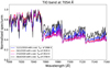 |
Fig. 3 TiO band at 7054 Å taken on four different dates: 11 November 2019 (blue), 24 January 2020 (red), 27 February 2020 (magenta), and 26 April 2020 (black). |
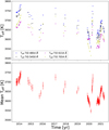 |
Fig. 4 Effective temperature time series obtained from TIGRE/HEROS spectra: upper panel: effective temperatures obtained from four TiO bands. Lower panel: respective averaged effective temperatures. |
4 Chromospheric activity
A well-known and commonly used indicator for stellar chromospheric activity is the line emission of the Ca II H&K doublet line at 3968.47 Å and 3933.66 Å, which is characterised by the so-called S -index. During the great dimming event of α Ori, our TIGRE observations show strong changes in the observed S -index, which we present in this section. These measurements, combined with historical Mount Wilson S-measures, provide a long-term time series for α Ori, which yields an interesting comparison to the available photometric data. Finally, we discuss the significant temperature impact on the S -values and present an analysis of the Ca II H&K fluxes in absolute terms.
4.1 Ca II K variation during the great dimming
Upon visual inspection of the Ca II K line spectra taken by TIGRE during the great dimming event we see a strong increase in the line core relative to the surrounding photospheric profile. For a closer comparison, all spectra were normalised to unity at the (photospheric) wavelength point 3925 A and 3942.32 A in order to give an equal relative scale to the Ca II K line cores of different observing dates.
In Fig. 5, we compare these normalised Ca II K line spectra taken on 29 January 2019 (TIGRE SII_MWO = 0.554), 11 November 2019 (TIGRE SII_MWO = 0.697), 24 January 2020 (TIGRE SII_MWO = 0.800), 27 February 2020 (TIGRE SII_MWO = 0.748), and 9 April 2020 (TIGRE SII_MWO = 0.601). In addition, the TIGRE spectrum of 11 January 2021 (SII_MWO = 0.492) serves as a reference for a Ca II K line core of low activity. This comparison, at face value, shows that the normalised Ca II K line flux increased until 24 January 2020 and thereafter decreased again. The same behaviour is seen in the measured S-values; the method for deriving S-values on the Mount Wilson scale is described in the following subsection (Sects. 4.2.2 and 4.2.3).
Furthermore, we want to draw attention to the fact that the spectrum around the K1V and K1R points is also variable; these points are marked in Fig 5, and form in the transition from photosphere to chromosphere (see Vernazza et al. 1981). These variations may indicate a changing photospheric contribution, which is consistent with the results of our temperature study of α Ori; see Sect. 3.
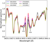 |
Fig. 5 Normalised Ca II K line spectra taken on different dates: 29 January 2019 (blue), 11 November 2019 (green), 24 January 2020 (red), 27 February 2020 (magenta), 9 April 2020 (black), and 11 January 2021 (yellow). |
4.2 S-index calculation for giants
The Mount Wilson program (described in detail by Wilson 1982) contains S -index measurements of giants. These were obtained with a wider bandpass filter for the line cores than the triangular bandpass with a FWHM of 1.09 A (used for main sequence stars) in order to accommodate, at least to some extent, the widening of the emission lines in giants (caused by the so-called Wilson Bappu effect). To compare the TIGRE raw S -index measurements of giants (SII_TIGRE) with the historical Mount Wilson data, the transformation onto the Mount Wilson scale was derived from a large set of observations of different giants with a wide bandpass, which were also observed by the Mount Wilson group.
4.2.1 The Mount Wilson S-index for giants
The commonly used Mount Wilson S -index is defined as (Vaughan et al. 1978)
 (1)
(1)
where NH and NK are the flux counts in the line cores of the Ca II H&K lines in a triangular bandpass with a FWHM of 1.09 A, and NH and NK are the flux counts of two 20 Å wide pseudo-continuum bandpasses, centred at 3901.07 Å and 4001.07 Å, which serve as a reference for the photospheric spectrum. In this fashion, the S -index value obtained is independent of the transparency of the night sky, and the factor α is merely a scaling factor (Vaughan et al. 1978; Duncan et al. 1991) used to compare different generations of master-built four-channel S -measurement units on Mount Wilson.
However, as already mentioned above, the Ca II H&K line cores of giant stars are wider than those of main sequence (MS) stars. Therefore, Wilson (1982) introduced a wider line bandpass for S -measurements of giants. This band pass has a trapezoidal shape with a FWHM of 1.5 Å and the top has a width of 1 Å. However, the wide continua bandpasses are the same as those used for the normal S -index (Choi et al. 1995). For our giant S -value measures on TIGRE spectra, we adopted a rectangular 2 Å line profile. This choice loses even less emission from supergiants than the Mount Wilson trapezoidal profile, and the calibrated transformation handles the different throughput.
Figure 6 shows the two different line-core bandpasses of the Mount Wilson S-indices plotted over a TIGRE spectrum of the Ca II K line of the giant HD 29139 (α Tau). The triangular bandpass is outlined by the black dashed line, and the wider trapezoidal bandpass by the red dashed line.
A visual comparison of both bandpasses shows that even the wider triangular bandpass is too small to capture the full line-core emission. Rutten (1984) provides a more detailed comparison and discussion of the S-values obtained with both of these bandpasses; his main conclusion is that the wider band pass for index SII_MWO becomes too narrow already for luminosity class (LC) I-II giants. The S -index can then only be used for variability monitoring, and is not useful for quantitative studies. We emphasise this point by superimposing the trapezoidal bandpass over the Ca II K line of a Ori, an LC I star, in Fig. 6.
4.2.2 The TIGRE SII-index for giants
We define the raw, uncalibrated TIGRE S -index for giants in the form
 (2)
(2)
where N* are the counts in the individual bandpasses. While we used the same continuum bandpasses (NR and NV) as for the Mount Wilson S -index, our TIGRE Ca II H&K line bandpasses (for NH and NK) are simply rectangular with a width of 2 Å (see Fig. 6). This choice gives the same width at the foot of the profile, but produces less count losses compared to the trapezoidal Mount Wilson profile.
Measuring the SII_TIGRE index requires three main steps, which are illustrated in Fig. 7. The first step concerns the values of the pseudo-continua, where the calibration fluxes N(R) and H(V) are measured. The standard normalisation process for TIGRE spectra may result in incorrect ratios between the fluxes of those reference bands. In the upper panel, a normalised TIGRE spectrum of the Ca II H&K lines is shown. A matching (by effective temperature and gravity) PHOENIX spectrum of models by Hauschildt et al. (1999) is now required to estimate the true flux ratios between the fluxes of those reference bands.
We normally use averages of the Teff and log g values in the PASTEL catalogue (Version 2020-01-30; Soubiran et al. 2016), except in the case of the variable effective temperature of α Ori. Instead, we adopt the values derived by our approach. According to those Teff and log g values, the corresponding PHOENIX spectrum is selected from the spectral database (Husser et al. 2013). To match the observed TIGRE/HEROS spectrum, we consider the rotational line-broadening (v·sin(i)) and a spectral resolving power of R ≈ 20 000 in the PHOENIX spectrum. The PHOENIX spectrum adapted in this way is then used to estimate the real spectral flux slope in the Ca II H&K region in the TIGRE spectrum; this approach was taken from Hall & Lockwood (1995) and guarantees consistency in the flux counts of the large reference bandpasses of the pseudo-continua, which form the denominator of the S -index.
The second step in deriving S II_TIGRE is the assessment of the exact RV shift of the Ca II H&K region of the respective spectrum by means of a cross correlation with the PHOENIX spectrum (see middle panel, Fig. 7). Subsequently, the TIGRE spectral fluxes are also re-normalised to the physical spectral slope seen in the PHOENIX spectrum (lower panel, Fig. 7). Fortunately, by the wise foresight of O. C. Wilson, the bandpasses of the S -index are symmetric, meaning that any remaining mismatches of the flux slope and the effective temperature are cancelled out in the resulting S -index.
Finally, the counts in the four bandpasses, depicted in the lower panel of Fig. 7, are obtained by integration, and the ratio between the sum of the two line bandpasses and the sum of the two continuum bandpasses is computed according to Eq. (2). The error estimation of SII_MWO follows the method used for STIGRE and described by Mittag et al. (2016). Indeed, apart from the continuum flux re-normalisation and line-core profiles, both indices are obtained in a very similar manner.
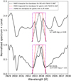 |
Fig. 6 TIGRE spectra of the Ca II K line of two giants (HD 29139 (LC III) and α Ori (LC I)) are shown with the line bandpasses of the different S-indices: The black dashed line outlines the triangular bandpass, sufficient in width for MS stars, and the red dashed line shows the wider trapezoidal bandpass used for giants. The magenta dashed line shows the rectangular bandpass used for the raw STIGRE index; see Sect. 4.2.2. |
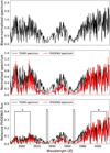 |
Fig. 7 Steps of the re-normalisation of spectra for TIGRE SII_MWO estimation: upper panel shows the Ca II H&K region of HD 29139 taken with TIGRE on December 27 2019; the middle panel shows the continuum-normalised spectra of the TIGRE spectrum as a black line and the selected and continuum-normalised PHOENIX spectrum as a red line, and the lower panel shows the re-normalised TIGRE spectrum as a black line and the PHOENIX spectrum in a relative flux scale (flux divided by the maximal flux). |
4.2.3 Transformation of SII_tigre to the Mount Wilson scale
The transformation between the TIGRE and the Mount Wilson giant S -index scales takes care of any instrumental effects. However, because of the large epoch difference, a larger number of giants needs to be considered to average out any individual changes in their activity levels. To do so, we chose giants both observed by TIGRE and contained in the Mount Wilson sample published by Radick & Pevtsov (2018). In total, we use 25 objects to derive the transformation, of which the SII_MWO values were measured by the present authors more than ten times.
These giants – with their physical parameters and median S -values, with the standard deviation of the median as error – are listed in Table 2. The rounded Teff and log g values are those of the selected PHOENIX reference spectra.
Figure 8 gives the distribution of SII_MWO vs. SII_TIGRE (average values) for all 25 giants. Here, a linear trend is very obvious and we derive the following transformation relation via an orthogonal distance regression, which is represented in the same figure by a solid line:
 (3)
(3)
which yields a standard deviation of the residuals of 0.024. In addition, we compute the percentage deviations (listed in Table 2) between the Mount Wilson reference S-values and the transformed TIGRE S-values, and obtain an averaged deviation of 5.6%. This is mainly an effect of long-term changes in the activity levels between the very different epochs of the observations, but is also attributable, to a much lesser extent, to observational error.
Giants used for the transformation of the SII_TIGRE into the Mount Wilson scale.
4.3 Long-term time series: Joining TIGRE and Mount Wilson S-index values
We now exploit the fact that the red supergiant α Ori is both part of our TIGRE giants observation program and contained in the Mount Wilson program (see Radick & Pevtsov 2018), with available data reaching back into the 1980s. These data allow us to examine whether or not a similar behaviour of the S -index as observed during the great dimming in the winter between 2019 and 2020 – with a simultaneous significant increase in the S -index anti-correlated with the V-band luminosity – has already occurred before.
The combined, long-term S -index time series is shown in the lower panel of Fig. 9. The Mount Wilson data are represented by black points and cover the period of September 1983 to March 1995. The TIGRE observation of α Ori started in September 2013 once TIGRE went into operation. Only S -index values based on spectra with an S/N larger than 25 at 4000 Å are shown (as blue points). In total, a period of 38 yr is covered, from 1983 to 2021, albeit with a gap of 18 yr between 1995 and 2013. As can be seen from Fig. 9, the median of the α Ori S-value is 0.539 over the whole period.
At least three episodes of strongly increased S -index values occurred during those 38 yr. The first one took place around 1984 with a maximum S-value of 0.7811 on 25 March, 1984, which is 45% larger than the long-term median S-value, with a phase of increased S -index level continuing until 1985. The second event took place in 1989 with a maximum S-value of 0.6879 on 1 October, 1989, which is 28% above the median S -index value. The third and most significant event is the ‘great dimming’ in 2020 with a maximum S -index value of 0.800 reached on 24 January, 2020, which is 48% larger than the median S-value of 0.539. To see whether the earlier two events are of a similar nature to the 2020 event, we now need to look at the correlation with photometric data.
4.4 Comparing S-index and photometric variations
The latest 2020 increase in S -index values showed a good anti-correlation and synchronisation with the great dimming event in 2020. To take a look further back in time, we again employ the photometric data taken from the AAVSO database. Figure 9 shows the light curve of the visual band magnitude in the upper panel, and the V-band magnitude (Johnson V-band) versus time in the middle panel. To ease this comparison, the above-mentioned periods of increased S-values are marked by dashed vertical lines. The visual magnitude light curve does show a dimming in 1985, slightly delayed against the maximum increase in S -index values around 1984. However, we caution that the decrease in the visual magnitude in 1984 and 1985 was established by only two observers and very few brightness estimates were made. However, the anti-correlation with the S-index supports the idea that we have an event similar to the great dimming in the winter between 2019 and 2020.
Unfortunately, V-band photometric data of before ≈ 1988 are quite rare, and so we need to use the more abundant visual magnitude estimates for our comparison with the older S -index time series. In the case of the S-increase around 1 October, 1989, the decrease in visual brightness is not as strong as during the 2020 great dimming event, but neither is the increase in S -index in 1989. From the few V-band data available, the brightness decrease can be confirmed and can therefore be considered as real. As mentioned above, the evidence for the 1984 and 1985 variation is less clear, yet there seems to be a recurrent pattern; namely that when the S -index rises, the visual brightness decreases. Such events last only o(1)yr, but lie several or even many years apart.
A simple explanation for this anti-correlation of S -index and V-mag lies in the definition of the S -index, according to which the near-ultraviolet (NUV) continuum fluxes of the reference windows form the denominator. As now seen very clearly in the recent great dimming event, when the brightness, and with it the temperature, decrease (see Gray 2008, Harper et al. 2020 and this work), the denominator of the S -index formula decreases, and consequently the S -index of α Ori increases, even if the chromospheric emission remains constant on an absolute scale. In addition, Dupree et al. (2020) present radial velocity data that indicate a variation of the stellar radius, adding to the effect of reduced continuum flux during such a dimming event. All these observations show that the photosphere of a Ori is not at all stable, and that in such a case the S -index is as sensitive to photospheric variations as it is to chromospheric emission changes.
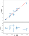 |
Fig. 8 SII_MWO vs. STIGRE transformation: upper panel: SII_MWO vs. SII_TIGRE. The solid line presents the transformation relation. Lower panel: residuals of the used transformation relation. |
4.5 The absolute scale: Ca II H&K flux
To obtain the true activity level of a Ori based on the S-index, the latter has to be transformed into physical emission line fluxes on an absolute scale. Given the photospheric variability, there is no single relation for a Ori to achieve this. Instead, we need to consider all components of S, the absolute NUV-continuum fluxes, and the line emission individually and for each spectrum separately.
To accomplish this we use the method developed by Linsky et al. (1979), which was originally designed to derive the absolute Ca II H&K flux for a Ori. However, this approach requires the removal of the instrumental and atmospheric effects on the spectral flux distribution. For this purpose, part of the TIGRE observing schedule on each night is an observation of at least one spectrophotometric standard star to create the instrumental (and atmospheric) response function for each night. Hence, for 73 a Ori spectra, we were actually able to obtain this spectrophotometric calibration.
After applying the nightly instrumental response function, the count ratio is calculated for observations with a sufficient S/N (larger than 25 at 4000 Å), following the definition by (Linsky et al. 1979), that is,
 (4)
(4)
where NH1 and NK1 are the spectral flux counts between the so-called K1 and H1 points of the Ca II H&K lines, respectively, and N3925-3975 is the count in a continuum bandpass of 50 Å in width centred at 3950 Å. In the case of a Ori, we assumed a distance of 3 Å between the K1 and H1 points. The positions of the K1 points of the Ca II K line are labelled in Fig. 5. The H1 point positions of the Ca II H line are similar to those for Ca II. In total, we were able to derive this count ratio IHK for 72 TIGRE spectra, which are shown in the upper panel of Fig. 10.
Not surprisingly, given the similarities in definition, the IHK time line shows a similar behaviour as the S -index values in Fig. 9. After all, both indices are based on a ratio between the flux counts in the H&K line cores and a UV reference continuum window, with the latter amplified by a change of the stellar radius, changing with a high power with decreasing effective temperature during the great dimming event.
To convert the IHK values into the absolute Ca II H&K fluxes, we then follow the relation given by (Linsky et al. 1979), that is,
 (5)
(5)
where, ℱ(Δλ) relation is given by Linsky et al. (1979):
 (6)
(6)
To do so, we perform a transformation of the effective temperatures (as derived above) into V – R colours using Eq. (C.1); see Appendix C. The result is shown in the middle panel of Fig. 10. Comparing these two panels, one immediately notices the entirely different behaviours of the two time series: while IHK-values (just like the S-indices) increase during the great dimming event, the derived absolute fluxes decrease, and their temporal behaviour is more comparable with that of the effective temperature (see Appendix A).
In this context, we must recall that some part of the H&K line-core emission is the underlying photospheric contribution, which – like the UV reference fluxes – strongly decreased during the great dimming event as well, driven by the decreasing effective temperature and the stellar radius. To evaluate the pure chromospheric activity of α Ori on an absolute scale, the latter has to be separated from the photospheric contribution and to be normalised by the corresponding bolometric flux.
This type of activity index was introduced by Linsky et al. (1979), who defined an  -index through
 (7)
(7)
A brief description of the estimation of photospheric flux (ℱHK.phot) is given in Appendix C, and the resulting  time series is presented in the lower panel of Fig. 10. Again, there is a remarkable difference compared to the two panels above. From the beginning of the dimming event to its brightness minimum,
  remains constant within its uncertainties. Then, with the recovery of the brightness of α Ori,
  (meaning the pure Ca II H&K flux, or line core ‘flux excess’) decreases. It therefore appears that any variation of the pure chromospheric emission, and so the magnetic heating, started only after the great dimming event had reached its full strength; however, given the large errors of
  , caused mainly by the uncertainty in the effective temperatures, this result has to be regarded with some caution.
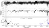 |
Fig. 9 Long-term time series: Comparison of the visual (upper) and V-band (middle) magnitudes of the AAVSO database with S-values of the Mount Wilson scale (lower panel). The dashed lines mark the periods with increased S-values. |
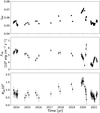 |
Fig. 10 Ca II H&K fluxes in relative and absolute flux scale: upper panel shows the count ratio IHK vs. time, middle panel the estimated absolute Ca II H&K flux, and the lower panel the estimated Ca II H&K flux excess |

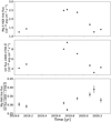 |
Fig. 11 Summed Mg II h&k spectral line flux (upper panel), the summed MUV fluxes in 2400–2700 Å (middle panel), both as obtained from Fig. 5 of Dupree et al. (2020), and their ratio (lower panel). |
4.6 The space view: Mg II h&k flux
Valuable additional observations of the chromospheric activity during the great dimming of α Ori were presented by Dupree et al. (2020), who performed measurements of spatially resolved Mg II h&k lines and MUV fluxes in 2400–2700 Å taken on eight different days in 2019 and 2020 with the HST/STIS. These data suggest a strong increase in flux in the period of 18 September to 28 November 2019, with a maximum on 6 October 2019.
Unfortunately, individual flux values are not listed in the paper by Dupree et al. (2020), but these values can be reasonably estimated (within their measurement uncertainties) from Fig. 5 of Dupree et al. (2020). The summed Mg II h&k line and summed MUV fluxes in 2400–2700 Å for each day, as well as their ratio, are shown here in the upper, middle, and lower panels of Fig. 11, respectively. As expected, the upper panel reproduces the increase in the Mg II h&k line emission described by Dupree et al. (2020); this is similar to the behaviour of our derived Ca II H&K fluxes over time (see middle panel of Fig. 10).
Forming the ratio of the Mg II h&k line emission over the MUV flux in 2400–2700 Å should then have a similar effect, as seen in the S -index and IHK time series, because in principle the photospheric flux part in the measured MUV flux in 2400–2700 Å, much like the UV flux in the reference bands of the S -index, is strongly temperature dependent.
Indeed, the lower panel of Fig. 11 does also show an increase in the Mg II h&k line flux relative to its MUV flux in 2400–2700 Å during the great dimming event. This demonstrates that there is no discrepancy between the observational evidence presented here regarding the chromospheric Ca II H&K line emission and the respective Mg II h&k data presented by Dupree et al. (2020). Both emissions should be, and indeed are, behaving in a very similar way during the great dimming event. The only difference is seen in the evidence for changes in the effective temperature, which is an issue we discuss below.
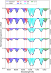 |
Fig. 12 Normalised spectra in the wavelength range from 6251 Å to 6263.4 A taken before, during, and after the great dimming event. The different colours mark the different elements and the red dashed lines indicate the laboratory wavelengths. |
5 Dynamical behaviour of the photosphere
We also detected significant variations and shape differences in other spectral lines: here we specifically focus on the wavelength range from 6251 Å to 6263.4 Å, which contains the V I 6251.82 Åand Fe I 6252.56 Å lines; the line-depth ratio of these lines depends on the effective temperature in cool giants (Gray & Brown 2001).
First, the spectra were normalised and RV corrected as described in Sect 5.1. In Fig. 12, we compare the normalised spectra taken before, during, and after the great dimming event to demonstrate the spectral changes. Figure 12 also demonstrates that the degree of blending of the involved spectral lines varies with time. To disentangle those changes, we performed a multiple Gaussian fit to better determine the true line centres as well as the width and the depth of each line; to ensure robust results we considered only low-noise spectra with a mean S/N of at least 100 in the considered wavelength range. From the derived true line centres, and using the laboratory wavelengths as listed in the NIST Atomic Spectra Database (Kramida et al. 2021), we then determined the respective rest frame RVs, which are presented in this section.
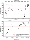 |
Fig. 13 Estimated RV values vs. time. The red dashed line marks the long-term average RV-value for α Ori of 21.56±0.58 km s−1 given by (Kharchenko et al. 2007). |
5.1 Mean RV variations
First, we had to determine a reference photospheric RV-value to which we compare each α Ori spectrum; for this, we used the line of Fe I at 6254.26 Å. The RV values for the other spectra were then determined by cross correlation with that iron line in the first spectrum, and we estimate the uncertainty of this procedure to be about ±0.4 km s−1 based on the assumption that the shift between two spectra can be determined with a sub-pixel accuracy of ±0.1 pixel.
In Fig. 13, we plot the resulting RV values. For the observing season between 2019 and 2020, these RVs are consistent with the RV values shown by Dupree et al. (2020). Additionally, we plot the average RV value of α Ori of 21.56±0.58 km s−1 given by Kharchenko et al. (2007), in order to better visualise the RV variations. As evident from Fig. 13, the RV variations range from ~14 km s−1 to ~26 km s−1, and we note that for the observation season from 2020 to 2021, the RV values are larger than the long-term average RV, except for the first two values, indicating a redshifted photosphere until the end of the year 2020. Subsequently, the RV values decrease until approximately 2021.1 and we see a blueshifted photosphere; later, the RV values increase again.
5.2 Line RV variations
Visual inspection of the spectra, as shown in Fig. 12 reveals some variations of the line centres. Some are blueshifted and others are redshifted. These variations include shifts of one line core with respect to another, suggesting anon-uniform motion of their slightly different geometrical origins.
In order to gauge the reality of this dynamical picture, we first checked the stability of the wavelength solution of our TIGRE spectra in this wavelength range. To do so, we determined the line centres of various lines in this wavelength region with respect to the RV standard star of that night, which is always taken for quality-control purposes (cf. the TIGRE webpage3). Each line centre was determined via a multiple Gaussian fit, in the same way as done for comparing the α Ori lines to one another as described above.
With respect to the RV standard stars, we find no significant trends in the lines cores, confirming the stability of our wavelength solution. The standard deviation of the rest RV variation of the respective lines (with a line depth of at least one-tenth of the normalised continuum) suggests a small scatter, ranging from 0.07 km s−1 for the Fe I line at 6254.26 Å to 0.55 km s−1 for the Ti I line at 6261.10 Å. We also checked in this fashion the stability of the line distances; here, we find a scatter of less than 0.02 Å.
Following this quality check, we restricted our analysis to spectra with rest-frame RV errors of below 2 km s−1, and considered only RV data more recent than epoch 2019.5, because the earlier observing cadence was not sufficiently dense. The derived time series of rest-frame RV (hereafter, rest RV) values of the V I at 6251.82 Å, Fe I lines at 6252.56 Å and 6254.26 Å, Ti I line at 6261.10 Å, and La II line at 6262.30 Å are shown in Fig. 14. In these time series, we observe some residual variation in the rest RV values. Also, these time series show a different trend in the rest RV values. To check whether these variations could be caused by residual errors in the wavelength solution of the TIGRE Échelle spectra, we check the line distances in this wavelength range in the RV standard stars observed on the same nights. Here, we do not find any significant scatter in the line distances and therefore we conclude that the observed variations are not caused by an erroneous wavelength solution.
To visualise the different trends in the time series of the rest RV values, we computed the rest RV differences for four line combinations and list our results in Table 3; to this end, we normalised the rest RV by subtracting the mean rest RV value and computed the differences of these rest RV values. These RV differences (ΔRVnorm_rest) values are shown in Fig. 15, which demonstrates a clear wave-like variation in the time range 2019.5–2020.5 during the great dimming. Figure 15 also shows that the variations during the great dimming were much stronger than those observed during the following season. To quantify the strength of these variations, the standard deviation of these variations is computed for these two observation epochs and also for both individual seasons, with the results being listed in Table 3.
In summary, we exclude that the variations in the rest RV values are an artifact created by an uncertain wavelength solution. Rather, we assume these variations to be a sign of additional motions, suggesting that the behaviour of the variations in the rest RV values indicates a difference in motion between the mean regions where the different lines are formed.
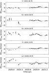 |
Fig. 14 Rest RV values over observing epoch. The grey area marks the range of the scatter as expected from the line RV examination with respect to the RV standard stars. |
Standard deviations of the difference of the rest RV values for different line combinations.
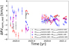 |
Fig. 15 Normalised rest RV value vs. time. The different signs and colour codes mark the different line pairs. |
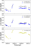 |
Fig. 16 Line depths vs. time shown. |
5.3 Variation of the line depths and widths
The strong line variability during the great dimming event is evident from Fig. 12. To visualise this significant variation in lines, we plot the line depths and the line widths obtained from the Gaussian fits against observing epoch in Figs. 16 and 17 for the lines of Fe I at 6252.56 Å and 6256.36 Å, the V I lines at 6251.82 Å and 6256.90 Å, and for the Ti I lines at 6261.10 Å.
Both line parameters show clear variations with a wave-like shape reminiscent of the effective temperature time series shown in Fig. 4. Furthermore, the strengths of the variations in the line depths are about the same, while the strengths of the variations in the line widths are clearly different. The differences in the variation of the line widths indicate differences in the extent of thermal broadening between the respective mean regions of the respective line origins. Again, the variations in depth and width of the lines presented here suggest that the photosphere is always dynamic; however, during the great dimming event, the resulting changes were extraordinarily large.
5.4 Temperature sensitive line-depth ratio of V I 6251.82 Åover Fe I 6252.56 Å
Gray & Brown (2001) demonstrated that the line-depth ratio (LDR) of the lines of V I at 6251.82 Å and Fe I at 6252.56 Å can be used to estimate the effective temperature for cool giants. The LDR is determined by the expression
 (8)
(8)
Gray (2008) used this LDR to study the variations of α Ori and showed it to correlate with the V magnitude. However, Gray (2008) thought that a conversion of the LDR values into α Ori temperatures is not possible in absolute terms in the absence of an established relation. However, it is plausible that such a relation exists in physical terms, as we see below.
In this work, we measured the LDR of the V I 6251.82 Å and Fe I 6252.56 Å lines to see whether any significant variations occurred during the great dimming event and how these compare to the normal variations of α Ori. For this purpose, we used the line depths obtained from the amplitudes of the Gaussian line fits above to compute the depth ratios of these lines; we show our results in Fig. 18. We see that the LDR values do indeed vary with time and behave much like our derived effective temperature; see Sect. 3.2.
These results suggest a consistent relation between our effective temperature values and the LDR (see Fig. 19), with a simple linear behaviour, which is represented in the same figure by the solid line:
 (9)
(9)
The scatter of this relation is small: we obtain a standard deviation of the residuals of only 24 K.
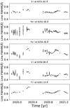 |
Fig. 17 Line FWHM vs. time shown. |
6 Summary and conclusions
In this study, we performed a multi-wavelength analysis of the variations observed during the great dimming event of α Ori and in the subsequent observation season of 2020–2021. To provide an overview, we plot the derived time series of the V magnitude, the well observed and temperature-dependent colour index R − I, our effective temperature values, the RVrest km s−1 of the line-core variation, our S-index time series, the derived  values, and the ratio between the absolute Mg II h&k line flux and the MUV flux in 2400–2700 Å shown in Dupree et al. (2020) in Fig. 20; as a reference of the long-term variability, the values of the V-band magnitude are instructive and therefore, we show them here in the upper panel of Fig. 20.
Clearly, the values of effective temperature are important for a complete understanding of the chromospheric activity of α Ori in absolute terms. We analysed the variations in different colour indices using the photometric data of the AASVO, as well as of the LDR of the V I 6251.82 Å and Fe I 6252.56 Å lines; as an example, we refer to the R − I index time series in the third panel of Fig. 20. This and the LDR time series do indicate changes in the effective temperature, especially during the great dimming event. To assess the effective temperature and its changes, we use four TiO bands covered by the TIGRE spectra and derive clear temperature variations of α Ori over time, in full agreement with Harper et al. (2020).
Next, we study the magnetic activity of α Ori, starting with the Ca II K line during the great dimming event. We find a strengthening of the chromospheric line-core emission relative to the photospheric spectrum in the months leading up to the brightness minimum, and afterwards a weakening of the relative Ca II K line-core brightness. We then compare the wider 2 Å S -indices taken with TIGRE with the respective values obtained by the Mount Wilson program in the 1980s for giants, including α Ori. To this end, we needed to derive a transformation equation between those two scales based on a larger number of giants observed by the present authors and Mount Wilson in order to average out most individual activity changes between those two epochs. Our analysis then shows that the current TIGRE measurements of the Ca II lines can be related to Mount Wilson S -index data taken much earlier and to the photometric data available from the AAVSO database over the past four decades. We used these relations to construct a long-term light curve of α Ori that extends over almost 40 yr, thus providing a very much extended perspective of the great dimming event.
Upon subsequent inspection of the combined 2 Å S-index time series, we note three larger increases in the S-values, each lasting less than a year, occurring in 1984−1985, 1989 (both Mount Wilson data), and 2020 (TIGRE); the latter coincides with the great dimming event and is shown here in the fifth panel of Fig. 20. A comparison with the V-band light curve shows a clear brightness decrease over the same period, suggesting a correlation between the decrease in brightness and the increase in the S-values. This correlation indicates that the debated former dimming in 1984 and 1985 was a real event – even though only two observers recorded this event in the visual band – because it coincided with the first 2Å S-increase observed by Mount Wilson.
Next, we estimated the Ca II H&K line flux in absolute terms, applying the method by Linsky et al. (1979) to α Ori. The time series of the absolute Ca II H&K line flux obtained in this way shows, in stark contrast to the S-value time series, that at the beginning of the great dimming event there was clearly a larger chromospheric emission than at the brightness minimum. The time series rather follows the shape of the effective temperature graph during the great dimming, which is no surprise, because the continuum flux – used as a reference to estimate the line flux – depends very strongly on the effective temperature in this NUV spectral range. Ignoring this effect would be like comparing the fluxes of two different stars, because the effective temperature of α Ori changes notably during the great dimming event.
We also estimated the excess of the normalised Ca II H&K line flux,  . Interestingly, this excess flux does not change significantly at the beginning of the great dimming event (see sixth panel of Fig. 20), and only starts to vary after the dimming event. Also, comparing the absolute Ca II H&K line flux with the absolute Mg II h&k line flux, our results and those of Dupree et al. (2020) are comparable. We therefore conclude that in order to remove the temperature effect on the latter, we need to involve the ratio between the absolute Mg II h&k line flux and the MUV flux in 2400−2700 Å (shown in Dupree et al. 2020; see Fig. 11 and the seventh panel of Fig. 20). This ratio shows a behaviour that is comparable to that seen in our
  time series during the great dimming.
This finding implies that the chromospheric activity did not change much at the beginning of the observed brightness minimum; however, as seen in the time series of  , there is a decrease in chromospheric activity after the brightness minimum in February 2020. Therefore, our interpretation contradicts that of Dupree et al. (2020), at least as far as the cause of the dimming is concerned. Whatever started this chain of events does not seem to be located in the outer atmosphere.
This conclusion is supported by the observed variations in different lines, which display strong changes during the great dimming event, both in their ratio of line strength, which are caused by the impact of the effective temperature changes, and also in their width and respective RV; an example is shown in the fourth panel of Fig. 20. This dynamical behaviour indicates a strong variation in the photosphere of α Ori.
In agreement with previous studies, our results demonstrate that α Ori is a highly variable star, which is reflected in all parameters illustrated in Fig. 20. This leads us to the interesting question of how these variations provide support to the two main hypotheses for the cause of the great dimming event. The decrease in the mean effective temperature, as demonstrated here, in combination with a reduction in the effective luminous area of the photosphere – which may not necessarily be a radius change – supports scenarios (see Freytag et al. 2019) where a large cool area forms temporarily, while a much smaller number of warm convection cells rise. Such temporary quasi-synchronisation of several large convection cells may go hand in hand with shock- or density waves. The down-flow of such a large, temporary cool area, which greatly reduces both the effective luminous area of the photosphere and the effective temperature, would not appear as obvious changes in RV; cooler regions are under-represented in the observed line profiles, because cooler gas contributes much less to the total emergent flux, and we would rather expect changes on a differential scale between lines with different formation temperatures, as reported here. Thus, all these ideas point to the photosphere and its convection as the main driver of the great dimming event.
The other prominent hypothesis, put forward by Dupree et al. (2020), assumes veiling by dust related to an observed mass ejection in October 2019. This idea is also based on the stronger absolute Mg II h&k line flux and MUV flux in 2400−2700 Å seen in October 2019 compared to the respective fluxes during the brightness minimum in February 2020 reported by the same authors. In our study we too find that the absolute Ca II H&K line flux was clearly larger in November 2019 than during the brightness minimum in February 2020. However, the significant changes in effective temperature and luminous area must be accounted for in order to correctly assess the chromospheric energy output on an absolute scale as shown above. As a consequence, the apparent large chromospheric emission increase that was observed to take place simultaneously with the beginning of the great dimming event disappears, and it is not until after the bolometric brightness minimum that the chromosphere reacts to it in absolute terms.
Thus, the corrected timing of the different events disagrees with the assumption of a strong mass ejection in October 2019, and any subsequent veiling by dust is therefore an unlikely cause of the great dimming; it would rather be a consequence and serve as an enhancement. Further evidence in favour of an origin of the chain of events in the photosphere and its convection, forming sometimes larger cool plumes, is provided by the recurrence of such an event; we show the similarities between the available data from 1984−1985 and those from 2020−2021. Given the extremely large size and therefore small number of convection cells under the extremely low gravity of α Ori, any temporary chance synchronisation and plume formation on the earth-facing side should indeed not be a particularly unique event.
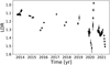 |
Fig. 18 Time series of the line-depth ratio of the V I 6251.82 Å and Fe I 6252.56 Å lines. |
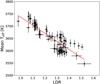 |
Fig. 19 Teff over the line-depth ratio. The solid line represents their mean relation. |
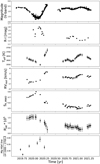 |
Fig. 20 Summary of the time series to show the main variation results. From top to bottom, we show the V-band, R – I colour index, the effective temperature, the RVrest variation of the Ti I line at 6261.1 A and the TIGRE SII_MWO, the |

Acknowledgements
We are grateful to our anonymous referee for the kind report. We particularly wish to thank our colleague Bernd Freytag of the Theoretical Astrophysics Department, Uppsala University, for enlightening discussions of how to interpret the complex information gained from our observations. We particularly acknowledge use of the public HK_Project_v1995_NSO data base of the Mount Wilson Observatory HK Project, which was supported by both public and private funding through the Carnegie Observatories, the Mount Wilson Institute, and the Harvard-Smithsonian Center for Astrophysics, running from 1960ies over more than three decades. These data are the result of the dedicated work of O. Wilson, A. Vaughan, G. Preston, D. Duncan, S. Baliunas, and many others. We are also very grateful for using the AAVSO International Database, photometric data on α Ori contributed by observers worldwide. Furthermore, the VizieR catalogue access tool, CDS, Strasbourg, France (see the original description of the VizieR service: A&AS, 143, 23) was helpful to this research, as well as the SVO Filter Profile Service (http://svo2.cab.inta-csic.es/theory/fps/) supported from the Spanish MINECO through grant AYA2017-84089. Finally, our research and international collaboration between Germany and Mexico, as well as the operation of TIGRE, has benefited significantly from travel money by the Conacyt-DFG bilateral projects No. 207772 and 278156, and by the institutional support given by the universities of Hamburg and Guanajuato (UG: by DAIP funding from its project 003/2022 and CAP programs) over the past decade.
Appendix A Variation of the calculated radius and calculated log(g)
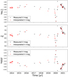 |
Fig. A.1 Calculated stellar properties where BC is constant vs. time: Upper panel: Logarithmic luminosity in solar units vs. time. Middle and lower panels: Calculated radius in solar units and calculated gravity (calculated log(g)) on the same timescales. Here, a constant BC of -1.93 was used, which is based on the long-term mean effective temperature. |
Dupree et al. (2020) presented RV measurements of α Ori during the great dimming event. These were variable and are correlated with the observed V mag variation. If there are real radius changes, the question therefore arises as to which changes we address here in terms of the calculated radius. Indeed, the photometric variation cannot be explained by the effective temperature changes alone and implies changes in the calculated radius. However, we cannot distinguish whether these reflect physical radius changes or simply changes in the effective luminous area. A reduced calculated radius could also result from the temporary presence of a large dark patch on the photosphere, such as that seen when there is a rising or sinking cooled plume formed in the course of some chance synchronisation of the few large granules on the observable side of this supergiant.
To estimate such changes in the stellar radius of α Ori in absolute terms, the luminosity of α Ori can be used: assuming spherical symmetry, it is proportional to  . For a quantification of the stellar luminosity of α Ori, we adopted the distance of 168 pc given by Joyce et al. (2020). In addition, we used the V magnitude data from the AAVSO database of the days where we were able to derive an effective temperature.
For days with an effective temperature value but no V mag, we interpolated the nearest V mag data. The results of this calculation are shown in the upper panel of Fig. A.1. For simplicity, the bolometric correction (BC) of -1.93 mag here is based on the long-term mean effective temperature of 3649 K, but see below. For the calculation of the latter, we apply Eq. 10.10 of Gray (2005).
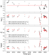 |
Fig. A.2 Calculated Stellar properties where BC is variable vs. time: Upper panel: Time-variable BC, using the derived daily effective temperatures (black dots). The red dashed line shows the BC of the mean effective temperature of 3649 K. Second panel: Logarithmic luminosity. Third panel: Stellar radius. Lowest panel: log(g). Black points represent the values obtained with daily, time-variable BC (as in the top panel), and red points show the values using the constant BC instead. |
The strong decrease in the stellar luminosity during the great dimming event is obvious, and radius and gravity values calculated from luminosity and effective temperature are presented in the middle and lower panels of Fig. A.1. As the luminosity drop was too large to be explained by the lower effective temperature alone, the radius would had to decrease from ≈640 R⊙ on 11 November 2019 to ≈500 R⊙ on 24 January 2020, which would explain the above-mentioned variation of the RV data.
The log(g) values were then calculated using the above stellar radius values and assuming a (constant) mean stellar mass of 17.75 M⊙ (see Joyce et al. (2020)). As seen in the lower panel of Fig. A.l, there is an increase in the calculated log(g) of up to ~0.3 dex during the great dimming event, which is caused by the reduction in calculated radius.
In this context, the impact of the temperature variation on the bolometric correction (BC) now requires some consideration. For this purpose, we calculated the BCs for the individual days (see top panel of Fig. A.2) where we had derived the effective temperature, again using the relation in Eq 10.10 of Gray (2005). We repeated the calculation of the luminosity, radius, and gravity to assess the impact of a time-variable BC (in the range of -1.69 mag to -2.26 mag) and compared the results with those obtained assuming a constant BC (-1.93 mag) based on the long-term mean effective temperature of 3649 K. These comparisons are shown in Fig. A.2.
The second panel of Fig. A.2 shows the logarithm of the luminosity in solar units versus time, the third panel depicts the calculated radius, and the lowest panel the calculated log(g) (if the calculated radius was indeed representative of the geometrical radius). In all panels, black points represent the values calculated with the time-variable BC based on the daily effective temperatures, and red points depict the values for which the constant BC of the long-term mean effective temperature is used.
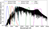 |
Fig. B.1 Normalised PHOENIX spectrum (Teff = 3600 K, log(g) = 0 and [Fe/H] = 0),; over-plotted are the filter functions used here. |
Not surprisingly, we find some differences between the use of the daily time-variable BC and a constant mean effective temperature BC for the stellar luminosity, calculated radius, and calculated log(g). In principle, these differences vary with the course of the effective temperatures and amplify the effect of the latter on all three quantities. From this test, we conclude that all the consequences of the effective temperature changes must be considered.
Appendix B Theoretical colour estimation using PHOENIX model spectra
To understand, at least qualitatively, the non-linear behaviour of the different colour indices B − V, V − R, R − I, and J − H mag with a variable effective temperature in the range from 3300 K to 4000 K, we estimated these indices from synthetic PHOENIX model spectra of different temperatures. Here we give an example to our work, using the synthetic spectrum of the model atmosphere for Teff = 3600 K, log(g) = 0, [Fe/H] = 0, as made available by the University of Göttingen database of Husser et al. (2013).
The filter functions for the B, V, R, and I bands were taken from Mann & von Braun (2015), and for the J and H bands we used the Keck_NIRC2.J and Keck_NIRC2.H filter functions available from SVO Filter Profile Service4 (Rodrigo et al. 2012; Rodrigo & Solano 2020). The above-mentioned PHOENIX spectrum and these filter functions are plotted in Fig. B.1. To derive colour indices from the PHOENIX model, the synthetic spectral flux, weighted with the filter function, is integrated over each band, and then converted into magnitudes. For this last step, a theoretical spectral flux reference to a ‘white’ AO standard star, such as Vega, is required. We use the synthetic PHOENIX spectrum with the physical parameters Teff = 9600 K, log(g) = 4.0, and [Fe/H] = −0.5. The results of these estimations are shown in Fig. B.2. Regarding the colour indices, in general the colour index increases with decreasing effective temperature; however, as demonstrated in Fig. B.2, the values for the B-V colour index actually decrease with effective temperature once this latter drops below 3600 K.
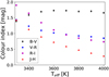 |
Fig. B.2 B − V, V − R, R − I, and J − H colour indices vs. effective temperature. |
 |
Fig. C.1 Continuum counts without the counts in the 3 Å bandpass of Ca II H&K lines vs. air mass. |
Appendix C Ca II H&K flux estimation
To estimate the Ca II H&K flux, we used the method described in Linsky et al. (1979) and the main points of this method are given in Sect. 4.5. Here, we want to add and discuss a few added details.
Appendix C.1 Spectrophotometry: counts of a 50 Å continuum window vs. airmass
For the Ca II H&K flux estimation with the method described in Linsky et al. (1979), a spectrophotometric standard star is required to create an instrumental response function. Unfortunately, the air mass of the target star and the observed spectrophotometric standard star can be different, and so can the extinction, which then causes a distortion or tilt of the derived spectral energy distribution (SED) of each flux-corrected spectrum. To test the impact of this problem, which should become worse at large airmass, we integrated the counts in the 50 Å bandpass window centred at 3950 Å (where the counts in the 3 Å bandpass of Ca II H&K lines are not considered). These continuum counts are plotted here against air mass; see Fig. C.1. Fortunately, we do not find any significant correlation between the flux-corrected continuum counts and the air mass, which suggests that this possible problem is sufficiently well controlled by our procedures.
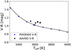 |
Fig. C.2 PHOENIX V − R vs. effective temperature : Blue points: V – R colours derived from PHOENIX spectra over effective temperature. The solid black line indicates the best-fit relation between the two. Black points: V – R colours from the AASVO database over our derived effective temperatures from different days in the time line. |
Appendix C.2 V – R colour index–Teff relation
In the conversion of the count ratio (IHK, see Eq. 4), the flux depends on the colour index V – R; see Eq. 6. However, the AAVSO database does not contain V – R values for the same days for which we have TIGRE spectra. Furthermore, we did not have enough data to derive a relation between effective temperature and V – R value.
Therefore, we derived the V − R colour index from PHOENIX spectra of the University of Göttingen database of Husser et al. (2013) as explained above, using models of different effective temperatures with [Fe/H]=0.0 and a log(g)= 0.0; see Sect. B. Figure C.2 shows these V – R colours against the respective effective temperature, represented by blue points.
To derive the relation between V – R and the effective temperature, we performed a least-square fit through:
 (C.1)
(C.1)
where x is x = Teff – 3300[K]; this relation is represented by a solid black line in Fig. C.2.
To test the reality of the PHOENIX spectra V − R values and their dependence on effective temperature, we compare these with the observed V − R colours from the AASVO database, coinciding in time with some of the days (only 7) for which we could derive an effective temperature. These observed V − R values are shown as black points in Fig. C.2.
This comparison shows that the observed V − R values are slightly above their synthetic counterparts, but the latter still represent the relative changes with effective temperature quite well. We conclude that the V − R values derived from PHOENIX models and their synthetic spectra are slightly smaller than in reality, implying that the real Ca II H&K fluxes and flux excesses may be a little larger than stated here.
Appendix C.3 Photospheric flux
In the case of α Ori, it is essential to remove the photospheric flux contribution from the Ca II H&K line in order to study the true stellar activity and prevent this latter from mimicking a false degree of variation in stellar activity. Here, we give a brief description of how we derive that photospheric flux contribution, following Linsky et al. (1979), who considers its part between the Ca II K1 and H 1 points of the Ca II H&K lines. To estimate the photospheric flux contribution in the Ca II H&K lines in our TIGRE spectra, we used the a linear trend between Ca II K1 and H1 points of the Ca II H&K lines. These are illustrated for the Ca II K line in Fig. C.3. Here, the magenta solid line represents the linear trend which splits the line flux into the photospheric and chromospheric contribution. The grey area in Fig. C.3 below the solid magenta line specifies the photospheric line contribution, and the red area in Fig. C.3 above the magenta solid line shows the pure chromospheric line emission.
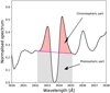 |
Fig. C.3 Ca II K line spectrum of α Ori. The magenta solid line shows the fit between the assumed K1V and KIR point. The grey area shows the photospheric contribution, and the red area represents the chromospheric emission. |
References
- Choi, H.-J., Soon, W., Donahue, R. A., Baliunas, S. L., & Henry, G. W. 1995, PASP, 107, 744 [NASA ADS] [CrossRef] [Google Scholar]
- Dharmawardena, T. E., Mairs, S., Scicluna, P., et al. 2020, ApJ, 897, L9 [Google Scholar]
- Duncan, D. K., Vaughan, A. H., Wilson, O. C., et al. 1991, ApJS, 76, 383 [Google Scholar]
- Dupree, A. K., Strassmeier, K. G., Matthews, L. D., et al. 2020, ApJ, 899, 68 [Google Scholar]
- Freytag, B., Höfner, S., & Liljegren, S. 2019, IAU Symp., 343, 9 [NASA ADS] [Google Scholar]
- González-Pérez, J. N., Mittag, M., Schmitt, J. H. M. M., et al. 2022, Front. Astron. Space Sci., 9, 912546 [CrossRef] [Google Scholar]
- Gray, D. F. 2005, The Observation and Analysis of Stellar Photospheres (Cambridge: Cambridge University Press) [Google Scholar]
- Gray, D. F. 2008, AJ, 135, 1450 [Google Scholar]
- Gray, D. F., & Brown, K. 2001, PASP, 113, 723 [NASA ADS] [CrossRef] [Google Scholar]
- Guinan, E. F., Wasatonic, R. J., & Calderwood, T. J. 2019, ATel, 13341, 1 [NASA ADS] [Google Scholar]
- Hall, J. C., & Lockwood, G. W. 1995, ApJ, 438, 404 [NASA ADS] [CrossRef] [Google Scholar]
- Harper, G. M., Guinan, E. F., Wasatonic, R., & Ryde, N. 2020, ApJ, 905, 34 [Google Scholar]
- Hauschildt, P. H., Allard, F., & Baron, E. 1999, ApJ, 512, 377 [Google Scholar]
- Hempelmann, A., Mittag, M., Gonzalez-Perez, J. N., et al. 2016, A&A, 586, A14 [NASA ADS] [CrossRef] [EDP Sciences] [Google Scholar]
- Hog E., Bastian U., Egret, D., et al. 1997, The Hipparcos and Tycho Catalogues (ESA Publications) [Google Scholar]
- Husser, T. O., Wende-von Berg, S., Dreizler, S., et al. 2013, A&A, 553, A6 [NASA ADS] [CrossRef] [EDP Sciences] [Google Scholar]
- Joyce, M., Leung, S.-C., Molnár, L., et al. 2020, ApJ, 902, 63 [Google Scholar]
- Kafka, S. 2021, Observations from the AAVSO International Database, https://www.aavso.org [Google Scholar]
- Kharchenko, N. V., Scholz, R. D., Piskunov, A. E., Röser, S., & Schilbach, E. 2007, Astron. Nachr., 328, 889 [Google Scholar]
- Kramida, A., Yu. Ralchenko, Reader, J., & and NIST ASD Team 2021, NIST Atomic Spectra Database (ver. 5.9), https://physics.nist.gov/asd [2021, December 29] [Google Scholar]
- Lançon, A., Hauschildt, P. H., Ladjal, D., & Mouhcine, M. 2007, A&A, 468, 205 [NASA ADS] [CrossRef] [EDP Sciences] [Google Scholar]
- Levesque, E. M., & Massey, P. 2020, ApJ, 891, L37 [Google Scholar]
- Linsky, J. L., Worden, S. P., McClintock, W., & Robertson, R. M. 1979, ApJS, 41, 47 [NASA ADS] [CrossRef] [Google Scholar]
- Mann, A. W., & von Braun, K. 2015, PASP, 127, 102 [NASA ADS] [CrossRef] [Google Scholar]
- Mittag, M., Hempelmann, A., González-Pérez, J. N., & Schmitt, J. H. M. M. 2010, Adv. Astron., 2010, 101502 [CrossRef] [Google Scholar]
- Mittag, M., Schröder, K. P., Hempelmann, A., González-Pérez, J. N., & Schmitt, J. H. M. M. 2016, A&A, 591, A89 [NASA ADS] [CrossRef] [EDP Sciences] [Google Scholar]
- Montargès, M., Cannon, E., Lagadec, E., et al. 2021, Nature, 594, 365 [Google Scholar]
- Piskunov, N. E., & Valenti, J. A. 2002, A&A, 385, 1095 [NASA ADS] [CrossRef] [EDP Sciences] [Google Scholar]
- Radick, R., & Pevtsov, A. 2018, in HK_Project_v1995_NSO (Harvard Dataverse), https://doi.org/1S.791S/DVN/ZR16NT [Google Scholar]
- Rodrigo, C., & Solano, E. 2020, in Contributions to the XIV.0 Scientific Meeting (virtual) of the Spanish Astronomical Society (Barcelona: Spanish Astronomical Society), 182 [Google Scholar]
- Rodrigo, C., Solano, E., & Bayo, A. 2012, SVO Filter Profile Service Version 1.0, IVOA Working Draft 15 October 2012 (IVOA Documents) [Google Scholar]
- Rutten, R. G. M. 1984, A&A, 130, 353 [NASA ADS] [Google Scholar]
- Schmitt, J. H. M. M., Schröder, K.-P., Rauw, G., et al. 2014, Astron. Nachr., 335, 787 [NASA ADS] [CrossRef] [Google Scholar]
- Soubiran, C., Le Campion, J.-F., Brouillet, N., & Chemin, L. 2016, A&A, 591, A118 [NASA ADS] [CrossRef] [EDP Sciences] [Google Scholar]
- Vaughan, A. H., Preston, G. W., & Wilson, O. C. 1978, PASP, 90, 267 [Google Scholar]
- Vernazza, J. E., Avrett, E. H., & Loeser, R. 1981, ApJS, 45, 635 [Google Scholar]
- Wilson, O. C. 1982, ApJ, 257, 179 [NASA ADS] [CrossRef] [Google Scholar]
All Tables
Standard deviations of the difference of the rest RV values for different line combinations.
All Figures
|
Fig. 1 Light curves of the B, V, R, I, J, and H bands, beginning with 2018.5. The upper panel depicts the J and H magnitudes, and the lower panel shows the B, V, R, and I bands. |
| In the text | |
|
Fig. 2 Colour index time series. The top panel shows the B − V values, the second displays the V − R values, the third the R − I values, and the lowest panel depicts the H − J values. Black dots represent values with a relative error of lower than 2%, whereas red data points those lower than 5%. |
| In the text | |
|
Fig. 3 TiO band at 7054 Å taken on four different dates: 11 November 2019 (blue), 24 January 2020 (red), 27 February 2020 (magenta), and 26 April 2020 (black). |
| In the text | |
|
Fig. 4 Effective temperature time series obtained from TIGRE/HEROS spectra: upper panel: effective temperatures obtained from four TiO bands. Lower panel: respective averaged effective temperatures. |
| In the text | |
|
Fig. 5 Normalised Ca II K line spectra taken on different dates: 29 January 2019 (blue), 11 November 2019 (green), 24 January 2020 (red), 27 February 2020 (magenta), 9 April 2020 (black), and 11 January 2021 (yellow). |
| In the text | |
|
Fig. 6 TIGRE spectra of the Ca II K line of two giants (HD 29139 (LC III) and α Ori (LC I)) are shown with the line bandpasses of the different S-indices: The black dashed line outlines the triangular bandpass, sufficient in width for MS stars, and the red dashed line shows the wider trapezoidal bandpass used for giants. The magenta dashed line shows the rectangular bandpass used for the raw STIGRE index; see Sect. 4.2.2. |
| In the text | |
|
Fig. 7 Steps of the re-normalisation of spectra for TIGRE SII_MWO estimation: upper panel shows the Ca II H&K region of HD 29139 taken with TIGRE on December 27 2019; the middle panel shows the continuum-normalised spectra of the TIGRE spectrum as a black line and the selected and continuum-normalised PHOENIX spectrum as a red line, and the lower panel shows the re-normalised TIGRE spectrum as a black line and the PHOENIX spectrum in a relative flux scale (flux divided by the maximal flux). |
| In the text | |
|
Fig. 8 SII_MWO vs. STIGRE transformation: upper panel: SII_MWO vs. SII_TIGRE. The solid line presents the transformation relation. Lower panel: residuals of the used transformation relation. |
| In the text | |
|
Fig. 9 Long-term time series: Comparison of the visual (upper) and V-band (middle) magnitudes of the AAVSO database with S-values of the Mount Wilson scale (lower panel). The dashed lines mark the periods with increased S-values. |
| In the text | |
|
Fig. 10 Ca II H&K fluxes in relative and absolute flux scale: upper panel shows the count ratio IHK vs. time, middle panel the estimated absolute Ca II H&K flux, and the lower panel the estimated Ca II H&K flux excess |
| In the text | |
|
Fig. 11 Summed Mg II h&k spectral line flux (upper panel), the summed MUV fluxes in 2400–2700 Å (middle panel), both as obtained from Fig. 5 of Dupree et al. (2020), and their ratio (lower panel). |
| In the text | |
|
Fig. 12 Normalised spectra in the wavelength range from 6251 Å to 6263.4 A taken before, during, and after the great dimming event. The different colours mark the different elements and the red dashed lines indicate the laboratory wavelengths. |
| In the text | |
|
Fig. 13 Estimated RV values vs. time. The red dashed line marks the long-term average RV-value for α Ori of 21.56±0.58 km s−1 given by (Kharchenko et al. 2007). |
| In the text | |
|
Fig. 14 Rest RV values over observing epoch. The grey area marks the range of the scatter as expected from the line RV examination with respect to the RV standard stars. |
| In the text | |
|
Fig. 15 Normalised rest RV value vs. time. The different signs and colour codes mark the different line pairs. |
| In the text | |
|
Fig. 16 Line depths vs. time shown. |
| In the text | |
|
Fig. 17 Line FWHM vs. time shown. |
| In the text | |
|
Fig. 18 Time series of the line-depth ratio of the V I 6251.82 Å and Fe I 6252.56 Å lines. |
| In the text | |
|
Fig. 19 Teff over the line-depth ratio. The solid line represents their mean relation. |
| In the text | |
|
Fig. 20 Summary of the time series to show the main variation results. From top to bottom, we show the V-band, R – I colour index, the effective temperature, the RVrest variation of the Ti I line at 6261.1 A and the TIGRE SII_MWO, the |
| In the text | |
|
Fig. A.1 Calculated stellar properties where BC is constant vs. time: Upper panel: Logarithmic luminosity in solar units vs. time. Middle and lower panels: Calculated radius in solar units and calculated gravity (calculated log(g)) on the same timescales. Here, a constant BC of -1.93 was used, which is based on the long-term mean effective temperature. |
| In the text | |
|
Fig. A.2 Calculated Stellar properties where BC is variable vs. time: Upper panel: Time-variable BC, using the derived daily effective temperatures (black dots). The red dashed line shows the BC of the mean effective temperature of 3649 K. Second panel: Logarithmic luminosity. Third panel: Stellar radius. Lowest panel: log(g). Black points represent the values obtained with daily, time-variable BC (as in the top panel), and red points show the values using the constant BC instead. |
| In the text | |
|
Fig. B.1 Normalised PHOENIX spectrum (Teff = 3600 K, log(g) = 0 and [Fe/H] = 0),; over-plotted are the filter functions used here. |
| In the text | |
|
Fig. B.2 B − V, V − R, R − I, and J − H colour indices vs. effective temperature. |
| In the text | |
|
Fig. C.1 Continuum counts without the counts in the 3 Å bandpass of Ca II H&K lines vs. air mass. |
| In the text | |
|
Fig. C.2 PHOENIX V − R vs. effective temperature : Blue points: V – R colours derived from PHOENIX spectra over effective temperature. The solid black line indicates the best-fit relation between the two. Black points: V – R colours from the AASVO database over our derived effective temperatures from different days in the time line. |
| In the text | |
|
Fig. C.3 Ca II K line spectrum of α Ori. The magenta solid line shows the fit between the assumed K1V and KIR point. The grey area shows the photospheric contribution, and the red area represents the chromospheric emission. |
| In the text | |
Current usage metrics show cumulative count of Article Views (full-text article views including HTML views, PDF and ePub downloads, according to the available data) and Abstracts Views on Vision4Press platform.
Data correspond to usage on the plateform after 2015. The current usage metrics is available 48-96 hours after online publication and is updated daily on week days.
Initial download of the metrics may take a while.