| Issue |
A&A
Volume 692, December 2024
|
|
|---|---|---|
| Article Number | A189 | |
| Number of page(s) | 13 | |
| Section | Stellar atmospheres | |
| DOI | https://doi.org/10.1051/0004-6361/202450691 | |
| Published online | 12 December 2024 | |
In pursuit of precise Ca II H&K chromospheric surface fluxes
A gravity and temperature dependence
1
Instituto de Radioastronomía y Astrofísica, Universidad Nacional Autónoma de México,
Morelia
58090,
Mexico
2
Departamento de Astronomía, Universidad de Guanajuato,
Guanajuato
36023,
Mexico
★ Corresponding author; This email address is being protected from spambots. You need JavaScript enabled to view it.
Received:
12
May
2024
Accepted:
13
November
2024
Abstract
The emission lines of the Ca II H&K doublet present one of the most important channels of radiative cooling for the chromospheres of cool stars. Although most other line emissions (Mg II h&k and numerous iron lines) populate the far-UV and require a very competitive space-born observing time, the Ca II H&K lines in the optical UV are easily accessible by ground-based spectroscopy with relatively cheap instrumentation, and the observational data are plentiful. At the same time, in order to include realistic mechanical and magnetic heating, advanced chromospheric models now require radiative cooling losses in absolute terms and therefore call for a precise surface flux scale, which could be provided by matching a photospheric Ca II H&K line profile computed by photospheric models. However, a major obstacle here is the significant ambiguity in parameter space in the face of a very sensitive dependence of cool stellar optical UV surface fluxes on the effective temperature. Consequently, we have developed a rigorous method by which precise physical parameters, most notably the effective temperature, are first determined by ISPEC tools working on high signal-to-noise spectra and based on a suitable line list and reference continuum. However, crosstalk and navigation of multiple local chi-square minima (best solutions) in parameter space must be considered. Only with the optimal set of parameters is a single PHOENIX model calculated, which defines the spectral surface flux scale in the Ca II H&K line region. In this paper, we discuss the results of the absolute measurements of Ca II K line fluxes for 32 representative cool stars and the accuracy of this approach. Finally, we show a comparison of the Ca II K chromospheric fluxes with line widths, and a relation of chromospheric flux with effective temperature and gravity following the logarithmic form log FCa II = α′ log g + β′ log Teff + C′.
Key words: techniques: spectroscopic / stars: activity / stars: chromospheres / stars: fundamental parameters / stars: late-type
© The Authors 2024
 Open Access article, published by EDP Sciences, under the terms of the Creative Commons Attribution License (https://creativecommons.org/licenses/by/4.0), which permits unrestricted use, distribution, and reproduction in any medium, provided the original work is properly cited.
This article is published in open access under the Subscribe to Open model. This email address is being protected from spambots. You need JavaScript enabled to view it. to support open access publication.
1 Introduction
The discovery of chromospheric emission in the cores of the Ca II H&K doublet (λ = 3933.66 Å and 3968.47 Å in air) as an activity indicator was made 110 years ago. When examining their spectra of solar active regions and very strongly overexposed spectroscopic plates of Arcturus, Eberhard & Schwarzschild (1913) found in both cases enhanced emission in the line cores of the K line of calcium and concluded, by analogy, that Arcturus was an active star. Ironically, the opposite was concluded in the late 1970s and 1980s based on Arcturus’s notoriously weak X-ray emission (Linsky & Ayres 1978). Today, we recognize that each activity indicator has its limitations when applied to cool luminous giants. While chromospheric emission in the Ca II H&K region benefits from the contrast with the faint photospheric spectrum, the detection of coronal emission in the form of X-rays encounters significant challenges. These challenges arise from geometric and energetic constraints in evolved giants, where the disappearance of coronae and the burial of magnetic fields beneath dense chromospheric layers make X-ray emission an unreliable indicator of magnetic activity (see, e.g., Ayres et al. 2003; Schröder et al. 2018). As a result, relying solely on X-rays can lead to an underestimation of stellar activity in these stars.
The visual inspection of photographic spectra by Olin C. Wilson on the Mount Wilson Observatory and the introduction of a novel S-value to measure the stellar magnetic activity in the late 1960s have left tens of thousands of observations of the Ca II doublet (Wilson 1978). The S-value was measured by an electronic four-channel analogue amplifier using a mask on the spectrum with slits open to two 20 Å wide reference windows on either side of the Ca II doublet and with a 1 Å wide slit in each line core. Hence, chromospheric emission was measured relative to the adjacent pseudo-continuum and as such independently of the photometric quality of the night (see, for example, Duncan et al. 1991; Baliunas et al. 1995). Calibration was obtained on each night by the use of several calibration stars from a list of 42 stars with different activity levels that are known to have little variability. Needless to say, ground-based optical spectroscopy has allowed for decades-long monitoring of stellar activity at a minimal cost compared to satellite technology.
A recent improvement of efficiency and in cadence has certainly been introduced by the use of robotic telescopes, such as Telescopio Internacional de Guanajuato Robótico-Espectroscópico (TIGRE – HEROS Schmitt et al. 2014; González-Pérez et al. 2022), but use of the Mount Wilson S-value is still beneficial today because it allows one to compare current observations directly with the historic measurements of the Mount Wilson program and thus to probe the variation of stellar activity on a timescale of many decades. However, a careful calibration process must be followed using the same calibration stars as used by the group of Olin C. Wilson (see extensive work by Mittag et al. 2016). Nevertheless, the general chromospheric astrophysical understanding has mainly been driven by satellite technology, especially in the period of the 1970s to the 1990s, using Copernicus, the International Ultra-violet Explorer, and finally the high-resolution UV spectrograph on the Hubble Space Telescope. The obvious advantage of satellites is that their instrumentation delivers physical flux data in the sense that there are no photometric issues related to changing atmospheric transparency. In addition, the most favorable farUV can be used, where chromospheric emission lines stand out against the dark UV photospheres of cool stars.
Through the work of Ayres et al. (1975) and Basri & Linsky (1979), among hundreds of other papers from that epoch, it has become clear that magnetic and mechanical chromospheric heating processes are balanced by radiative cooling through the collisional excitation and radiative de-excitation of numerous atomic transitions, producing the observed emission lines. However, the absolute scales remain uncertain from an empirical perspective. Space data provide physical fluxes at Earth, but uncertainties in the stellar parameters limit the accuracy of the derived surface flux scale (see, e.g., Pérez Martínez et al. 2014), and ground-based Ca II spectra usually lack a precise scale for the spectral flux. The modeling of chromospheric heating by Fawzy & Cuntz (2018) for eps Eri and by Fawzy & Cuntz (2021) for 55 Cnc have renewed the demand for measuring radiative cooling in absolute terms. Such physical models of chromospheric heating suggest total heating surface fluxes on the order of 108−109 erg s−1 cm−2. However, a rigorous radiative transfer and a physical photosphere are not included in these models, which limits the meaningfulness of comparison with observed chromospheric emission lines (see, e.g., Cuntz et al. 2021, using the Ca II K emission line of 55 Cnc).
An obvious solution is to obtain an absolute scale for the spectral surface flux by matching synthetic spectra of the Ca II H&K region of PHOENIX (Hauschildt & Baron 2005) model photospheres (Pérez Martínez et al. 2014). The practical problem with this approach in the optical UV is the extreme dependence of the surface flux scale of cool stars on effective temperature, by a power of nearly ten. At the same time, photospheric Ca II line profiles match those observed for models of a range of parameters. A typical uncertainty arising for the effective temperature is 4–10% (Soubiran et al. 2016), which results in a 16–40% error on the Ca II H&K surface flux scale given its dependence on the fourth power of the effective temperature.
This paper presents a method to overcome this ambiguity of spectral modeling by employing a rigorous use of ISPEC (Blanco-Cuaresma et al. 2014a; Blanco-Cuaresma 2019), following and refining the procedure introduced by us in Rosas-Portilla et al. (2022), and using an ISPEC script developed by us that allows the process to be largely automated. As described below, by basing the parameter assessment on more than 200 lines in the less crowded red spectrum and carefully navigating the problems and ambiguities of spectrum synthesis with ISPEC, we reduce the uncertainty of the effective temperature to about 1.5% (70 K) and obtain a surface flux scale with reliability in absolute terms of about 10% using precise PHOENIX models.
2 Assessment of the physical parameters by strategic employment of synthetic spectra
2.1 The stellar sample and spectroscopic observations
We selected a homogeneous set of spectra of comparable quality from a sample of 32 well-known stars with spectral types G and K, luminosity classes I to V, and a wide range of surface gravities from 1.0 to 4.5 dex, while the values of effective temperature span from 3869 to 5992 K (see Table A.2 below). All the stars were observed with the 1.2 m robotic telescope TIGRE (located near Guanajuato, central Mexico), which is equipped with the HEROS echelle spectrograph (R ≈ 20 000 in a wavelength range from 3800 to 8800 Å). Averaged over the entire spectrum, TIGRE-HEROS produces good quality spectra with an S/N ~ 100 or more, which corresponds to an S/N ~ 50–70 in the Ca II H&K line region. The spectral coverage of HEROS is achieved by two separate cameras (named channel R and channel B for red and blue light) with a small gap of ~120 Å around 5800 Å (located on the blue side of the sodium D line). In this way, the channels are individually optimized for each wavelength region, while sensitivity and resolution remain nearly uniform. The information on the chromospheric Ca II H&K emission is obtained from the B channel, while the R channel is more suitable for spectral synthesis due to its better S/N.
We typically added two or three spectra on both channels to improve our measurements of Ca II K emission line fluxes. Strict quality control by eye was performed to remove anomalous differences between different observations. This approach allowed us to avoid the effects of electronic noise or underexposure on poor transparency nights while optimizing the S/N of each spectrum and therefore our emission line flux measurements.
As can be seen in the plots of the chromospheric Ca II K emission line profiles (see the data availability section), the stellar activity is mostly low to moderate. The rotational and turbulent velocities, including their variation across the sample, remain within the spectral resolution of TIGRE-HEROS, which is equivalent to 7.5 km s−1, except for the most active giants, whose rotation velocities exceed 8 km s−1 (see, e.g., Aurière et al. 2015; Table 3 therein).
2.2 Calculation of parallax-based gravities
When spectral synthesis techniques are applied to spectroscopic analysis, parameter determination is complicated by having to fit several parameters at the same time, as this approach causes a multitude of ambiguous best-fit solutions in the parameter space, depending on the choice of the initial values. These solutions are caused by the fact that one mismatched parameter can be compensated in its effect by the mismatch of others, a phenomenon called crosstalk, and thus the result is a still seemingly good representation of the observed spectrum. Therefore, information external to spectroscopic synthesis, such as parallax-based gravities, is vital to allow for testing and filtering of seemingly equivalent best-fit solutions.
Due to possible crosstalk with the effective temperature Teff, we first had to determine the surface gravity log g. To calculate parallax-based gravities, we used an iterative process involving Teff derived by spectral synthesis, as shown in Fig. 1, until the difference between the parallax-based gravity and its derivation by spectral synthesis was less than ±0.09, that is, the uncertainty of log g determined with our method (see Sect. 2.7).
In a first step, we derived the absolute visual magnitudes V via the Gaia DR3 parallaxes (Gaia Collaboration 2016, 2021), the publicly available photometry, and estimated stellar masses M⋆ using a preliminary analysis of its position in the Hertzsprung-Russell diagram (HRD) to find the matching evolution track. We used the apparent photometric magnitudes of the SIMBAD database in the visual band mV as well as the color index B − V. The parallaxes in milliarcseconds (and the distances in parsecs) were taken from the Gaia DR3 archive. We applied the parallax zero-point correction of Lindegren et al. (2021), using their published Python code. No interstellar extinction correction was applied considering that the distances of our sample stars are, on average, less than ~100 pc.
To determine the bolometric magnitudes, luminosities, and masses, we applied the bolometric corrections BC from Casagrande & VandenBerg (2014, 2018), for which Teff, log g, and metallicity [Fe/H] are required. As initial values (to be refined later), we used the average of Teff, log g, and [Fe/H] for each star from the PASTEL catalog (Soubiran et al. 2016). The luminosity in solar units was calculated using the relation log L = (4.81 − V − BC)/2.5, where we applied a solar visual absolute magnitude of 4.81 (Willmer 2018). The stars were located on an HRD (see Fig. 2) to determine the M⋆ using the MIST stellar evolutionary tracks (Dotter 2016; Choi et al. 2016) that were calculated with the Modules for Experiments in Stellar Astrophysics (MESA) code (Paxton et al. 2011, 2013, 2015, 2018). We considered an uncertainty for each stellar mass estimate of about 10%. Finally, the surface gravity of each star was calculated from the respective stellar luminosity, mass, and effective temperature as follows. If R⋆ is the stellar radius,
![Mathematical equation: $\[\log~ L \propto ~\log \left(R_{\star}^{2} T_{\text {eff }}^{4}\right) \propto ~\log \left(\mathrm{M}_{\star} g^{-1} T_{\text {eff }}^{4}\right).\]$](/articles/aa/full_html/2024/12/aa50691-24/aa50691-24-eq1.png) (1)
(1)
Therefore, if log g⊙ = 4.437 (in units of cgs) is the solar surface gravity, the surface gravity is given by
![Mathematical equation: $\[\log~ g=4.437+~\log \left(\frac{\mathrm{M}_{\star}}{\mathrm{M}_{\odot}}\right)-~\log \left(\frac{L}{L_{\odot}}\right)+4 ~\log \left(\frac{T_{\text {eff }}}{T_{\odot}}\right).\]$](/articles/aa/full_html/2024/12/aa50691-24/aa50691-24-eq2.png) (2)
(2)
The preliminary gravities determined by Eq. (2) were used to derive the effective temperatures by means of spectral synthesis (see below) while avoiding solutions with wrong gravity due to crosstalk with Teff (Schröder et al. 2021). Subsequently, the calculated parallax-based gravities were updated with these self-determined Teff values (see Fig. 1). We repeated this procedure iteratively for each star to finally refine Teff and log g as mentioned above. Furthermore, we also tested the reliability of our gravity determination using MIST evolutionary tracks (see Sect. 2.7 for more details). Table A.1 details the distances, magnitudes, physical parameters, and parallax-based gravities of all 32 stars used in this study.
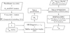 |
Fig. 1 Flowchart for determining the surface gravity log g. The term mV is the photometric apparent magnitude in the visual band, and B − V is the color index. The term V is the absolute magnitude in the visual band, BC is the bolometric correction, and L is the stellar luminosity. The term M⋆ is the stellar mass, and Teff is the effective temperature. |
2.3 Deriving effective temperatures by spectral synthesis
With the parallax-based gravities determined in the previous step, we then focused on determining Teff from the TIGRE-HEROS spectra using the spectral analysis tool kit ISPEC (Blanco-Cuaresma et al. 2014a) in its latest Python 3 version (v2023.08.04) (Blanco-Cuaresma 2019). ISPEC compares an observed spectrum with synthetic spectra interpolated from atmospheric models of different physical parameters using the least squares differences (χ2 method) to define the corresponding physical parameters. We developed SPARTAN (Stellar PARameter deTermination with Automatic Normalization – v1.1.3), a script for ISPEC written in Python 3, to perform the spectral synthesis with an algorithm that uses the very useful ISPEC tools in a consistent manner. The main features of SPARTAN are multithreaded execution, automatic radial velocity correction, automatic initial stellar parameter estimation using a precalculated synthetic grid, automatic continuum normalization (using synthetic continuum regions), and automatic search and filtering of good line-regions for the stellar parameter determination.
Given the better S/N of the R-channel (5800–8800 Å) compared to the B channel (3800–5680 Å) of the TIGRE-HEROS spectrum, we applied the spectral synthesis process only in this channel. In addition, the lower line density of the R-channel allowed us to avoid line blends that can interfere with the analysis. We used the grid of MARCS atmosphere models (Gustafsson et al. 2008) included in ISPEC, and for reference solar abundances, we used the values published in Grevesse et al. (2007). Synthetic spectra were calculated using the radiative transfer code TURBOSPECTRUM version 15.1 (Alvarez & Plez 1998; Plez 2012). This combination of radiative transfer code plus atmosphere models allowed us to have a better approach to the atmospheric conditions of cool giant stars.
However, residual mismatches of line strengths (atomic f-values) as well as subtle unnoticed blends with other lines can mainly cause a large minimal χ2 level (Schröder et al. 2021). Furthermore, non-local thermodynamic equilibrium (NLTE) effects may be mismatched by the model libraries that ISPEC can use toward the low end of stellar effective temperatures (see Sect. 3.1 for more details).
Preceding the spectral synthesis with ISPEC, continuum normalization of the observed stellar spectrum and line selection are necessary for the synthesis procedure. After several comparative tests, we found that the impact of this step on the final stellar parameters is not negligible since it affects the χ2 sums and their minima in parameter space.
The complications above impose limits and require careful handling of parameter evaluation. Our method for stellar parameter determination, in addition to being uniformly applicable to all sample stars, makes use of external information to spectroscopic synthesis, such as parallax-based gravities (see above), and it addresses the process of deriving effective temperatures using our ISPEC script, SPARTAN, which automates the spectrum normalization and selection of good spectral lines for reliable stellar parameter determination.
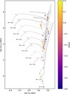 |
Fig. 2 Grid of evolution tracks with solar metallicity for different stellar masses in solar mass units. The color scale represents the metallicity of the star. We used MIST evolutionary tracks that were calculated with MESA. |
2.4 Guided spectral continuum normalization
We employed a synthetic spectrum that closely aligns with the observed spectrum to identify the appropriate continuum sections essential to direct the normalization process. To generate it, we used the preliminary initial values of Teff, log g, and [Fe/H] from the PASTEL catalog (see above). The resolution of the synthetic spectrum was adjusted to match the target spectrum of TIGRE-HEROS (R ~ 20 000). We maintained the projected rotation velocity v sin i at a low value of 1.6 km s−1, which is a reasonable choice for giants as well as for aged and relatively inactive main-sequence stars. Variations of a few kilometers per second in the rotational velocity are beyond the resolution capabilities of the TIGRE-HEROS spectra anyway. On the other hand, the micro- and macro-turbulent velocities for synthetic spectrum were defined using the approach in Rosas-Portilla et al. (2022) (see Eq. (A1), where the macro-turbulence velocity) vmac follows an empirical representation, according to the findings in main-sequence stars by Ryabchikova et al. (2016), while still using the micro-turbulence velocity vmic of the PHOENIX library (Husser et al. 2013) in this step.
Once the initial synthetic spectrum is created, the SPARTAN script automatically selects the continuum sections according to the following three criteria: (1) To avoid the accumulated effect of weak spectral lines, a maximum deviation of the relative intensity of the continuum section of 10% from unity is tolerated. (2) A minimal length of the section is set as equal to the full width half maximum of the instrumental profile of TIGRE-HEROS, that is, ~0.35 Å in the center of the R-channel and ~0.23 Å in the center of the B-channel. (3) Spectral regions with abundant telluric lines, that is, spectral lines created by Earth’s atmosphere and that can interfere with observations, were also discarded (Catanzaro 1997; Griffin 2000).
Finally, using the previously well-determined synthetic continuum sections, we normalized the observed stellar continuum by employing the ISPEC subroutine designed for this. The algorithm of ISPEC basically applies a third-degree spline with a median and a maximum filter (see Blanco-Cuaresma et al 2014a for more details). SPARTAN improves the ISPEC normalization subroutine in order to apply it only within our previously selected continuum regions. In addition, we designed the script SPARTAN to recursively repeat this process using different median and maximum filters, ten steps each from 0.1 to 1.0 Å for the former and 1.5 to 15 Å for the latter. A total of 100 possible normalizations are computed in parallel using multiprocessing capabilities.
SPARTAN identifies differences between synthetic and observed spectra, calculates the RMS strictly within continuous regions, and chooses the normalized spectrum with the best RMS. Finally, a second fine-tuning normalization is applied to the observed spectrum (see Rosas-Portilla et al. 2022 for more details). In general, this guided continuum normalization process substantially enhances the traditional by hand method. The principal advantage of our algorithm is its independence from any personal criteria when establishing the normalization regions of the spectral continuum (see an example of an automatically normalized spectrum in the data availability section).
2.5 Selection of key spectral lines for the synthesis process
The spectral synthesis process requires a representative and reliable subset of spectral lines that are less affected by line blends or mismatching atomic line strengths. In this work, the capabilities of SPARTAN described above allowed us to improve our previous selection in Rosas-Portilla et al. (2022) by avoiding lines within spectral regions that are known to host many telluric lines. In addition, we improved the cross-correlation algorithm between the observed line strength and the Vienna Atomic Line Database (VALD) list (Piskunov et al. 1995).
We performed spectral line selection to a high-quality solar spectrum taken by TIGRE-HEROS via the Moon’s reflection and based on our criteria (explained in detail in Rosas-Portilla et al. 2022, and references therein) while taking advantage of parallel computing capabilities of SPARTAN. From this process, a total of 202 lines were selected for the R-channel spectra of HEROS. Once again, our selection only considered spectral lines from iron peak elements (iron, chromium, and nickel) and alpha elements (silicon, calcium, and titanium; see the final list in the data availability section).
Our line selection was not used blindly in the observed spectra. In the same way as Blanco-Cuaresma (2019) and before starting the spectral synthesis process, SPARTAN checks if each line exists in the target spectrum. According to our tests, our spectral line selection worked well from main-sequence stars to supergiants.
2.6 Final stellar parameter determination
As a starting point, SPARTAN uses the initial Teff and [M/H] given by the average values found in the PASTEL catalog for each star to determine the stellar parameters from the normalized observed spectrum. The initial gravity is then calculated using Eq. (2). The initial vmic is set again using the PHOENIX library, while vmac is set by Eq. (A1) in Rosas-Portilla et al. (2022), and v sin i is maintained at an initial low value of 1.6 km s−1.
The exploration of the parameter space to determine the best-fit results given by ISPEC follows the strategy of Blanco-Cuaresma et al. (2014a), namely, varying the initial values in steps. However, the best-fit stellar parameters are sensitive to the choice of the initial parameters. SPARTAN implements an analysis that varies the initial parameters around the central value as follows: ±100 K for Teff, ±0.15 dex for log g, and ±0.15 dex for [M/H]. Including their combinations, SPARTAN executes a total of 27 iterations. Finally, the stellar parameters with the best χ2 result of all solutions are chosen.
SPARTAN includes the optimal method for determining stellar parameters, shown in detail in Rosas-Portilla et al. (2022) and Schröder et al. (2021). Namely, we vary only one parameter at a time and keep all other parameters constant (see the flowchart in the data availability section). Our script aims to minimize crosstalk by maximizing the use of non-spectroscopic information to exclude the best-fit solutions whose parameters contradict the information external to the synthesis process. Furthermore, SPARTAN takes advantage of multithreaded computing capabilities to accelerate the exploration of the parameter space and considers different possibilities for the initial values.
However, the values of vmic, vmac, and v sin i below 3 km s−1 have no physical meaning, considering the modest spectral resolution of the TIGRE-HEROS spectra, which are typically half the width of the instrumental line profile. Our results only demonstrate the reliability of the main physical parameters. Table A.2 summarizes the final stellar parameters obtained with this method and Fig. 3 shows a comparison between our results for Teff and [Fe/H] by spectral synthesis (as described above) and the average values in the PASTEL catalog for each star Figure 3 also shows a comparison between our results for log g by spectral synthesis using the script for ISPEC, SPARTAN, and parallax-based gravities.
2.7 Reliability test with Gaia FGK benchmark stars
We used a sample of eight well-known stars from the Gaia FGK benchmark stars (GBS hereafter, Jofré et al. 2014; Blanco-Cuaresma et al. 2014b; Heiter et al. 2015; Jofré et al. 2015; Hawkins et al. 2016; Jofré et al. 2017) to evaluate the reliability of the parameter determination method using the new features of the SPARTAN script as well as to determine whether the use of TIGRE-HEROS spectra could potentially influence our final results due to any instrument-related considerations.
Four of the eight stars used in our tests belong to the stellar sample used in this work. Following the same method in Rosas-Portilla et al. (2022), we tested the SPARTAN script with spectra of four different resolutions (instruments) and quality (S/Ns). Figure 4 shows the differences between the stellar parameters from the GBS library and SPARTAN script. After considering the standard deviation of the differences in the stellar parameters between the GBS and SPARTAN values, we finally concluded that the total uncertainty of the stellar parameters with this method are Teff = ±70 K, log g = ±0.09 dex, and [Fe/H] = ±0.08 dex.
In addition, we compared the parallax-based gravities derived using our method and the interpolated log g results of the MIST evolutionary tracks and PASTEL catalog entries. We find that the mean and standard deviation of the differences for parallax-based gravities versus MIST, ΔMIST = 0.15 ± 0.04, and versus PASTEL, ΔPASTEL = 0.15 ± 0.15, are quite comparable, probably due to the influence of metallicity interpolation on the evolutionary tracks. In contrast, the differences between the parallax-based gravities and our method using the SPARTAN script fall into ΔSPARTAN = 0.049 ± 0.024.
3 Chromospheric Ca II K emission line width and flux measurements
3.1 LTE versus Non-LTE
Stellar atmospheres are regions of high temperature and low density composed mainly of single atoms, ions, and free electrons and contain strong gradients in structural parameters. The nature of a stellar atmosphere – which is bounded by the stellar interior on one side and by a cool, essentially empty space on the other – prevents the microscopic state of the gas from being described by equilibrium thermodynamics. Instead, one has to use non-equilibrium statistical mechanics (Hubeny & Mihalas 2014).
The local thermodynamic equilibrium (LTE) is characterized by three equilibrium distributions: the Boltzmann excitation equation, the Saha ionization equation, and the Maxwellian velocity distribution of particles. In strict LTE, radiation and matter are assumed to be in equilibrium with each other throughout an atmosphere. Therefore, the source function is assumed to be given by the Planck function, and all atomic processes (excitation and deexcitation or ionization and recombination) are in detailed balance. However, the very fact that radiation escapes from a star implies that LTE must eventually break down at a certain point in the atmosphere.
By the term Non-LTE (NLTE), we describe any atomic state that departs from LTE. In practice, this usually means that populations of some selected energy levels of some selected atoms or ions are allowed to depart from their LTE value, while the velocity distributions of all particles are assumed to be Maxwellian, moreover, with the same kinetic temperature. In NLTE, radiation is no longer assumed to be in equilibrium with matter, and hence the full coupling between matter and radiation must be calculated in order to calculate the source function.
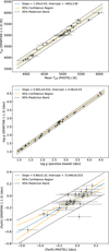 |
Fig. 3 Effective temperature, surface gravity, and metallicity comparison between the values calculated by spectral synthesis using the SPARTAN script and the average values in the PASTEL catalog. |
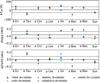 |
Fig. 4 Differences between the stellar parameters from GBS library and SPARTAN script. The mean values and standard deviations of the differences are ΔTeff = 28 ± 70 K, Δ log g = 0.04 ± 0.09 dex, and Δ[Fe/H] = −0.01 ± 0.08 dex. |
3.2 Photospheric synthetic models
Synthetic stellar spectra facilitate a comparison of the physics that we currently know of stellar atmospheres with direct observations of the studied stars. However, they are limited by the completeness of the spectral line lists and numerical assumptions (e.g., plane-parallel versus spherical geometry and LTE versus NLTE. In order to determine the structure of stellar objects, one must solve the radiation transport equation and compare synthetic spectra with observations.
Throughout its 30 years of continuous development, PHOENIX (Hauschildt & Baron 1999) has been a generalpurpose state-of-the-art radiative transfer code, and its purpose is to calculate atmospheres and spectra of stars across the HRD. PHOENIX allows us to include a large number of LTE and NLTE background spectral lines and solves the radiative transfer equation in spherical geometry, including the effects of special relativity in the modeling. Therefore, the profiles of spectral lines must be resolved in the co-moving (Lagrangian) frame. This requires many wavelength points (~15 0000 to 300 000 points). Since the CPU time scales linearly with the number of wavelength points, the CPU time requirements of such calculations are large. In addition, NLTE radiative rates for both line and continuum transitions must be calculated and stored at every spatial grid point for each transition, which requires large amounts of storage and can cause significant performance degradation if the corresponding routines are not optimally coded (Hauschildt & Baron 1999).
Figure 5 shows a comparison of a synthetic spectra for HD 124807 (Arcturus) in LTE and NLTE modes for two different wavelength regions, the H α line and the Ca II K line, as well as a spectrum observed with TIGRE-HEROS. The Arcturus spectrum in LTE and NLTE was calculated using the latest available version of PHOENIX v19.02.08B of July 2023. The spectrum in LTE was calculated using ~620 000 points, while for NLTE, ~3 500 000 points were used, and we considered the following elements in NLTE mode: H, He, Mg, Ca, and Fe. The spectrum computation in LTE mode took ~2.5 hours, and for NLTE mode, it took ~14.2 hours, each with 25 iterations.
It is clear that the difference between LTE and NLTE modes in the wavelength range of interest in this work, that is, the K line of Ca II, is minimal compared to the H α line. Therefore, we calculated our library considering the reliability and computing speed of synthetic spectra in the LTE mode. In addition, generating a library of synthetic spectra in NLTE would have taken a long time and would not guarantee a noticeable difference in our results.
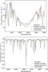 |
Fig. 5 Comparison of the synthetic stellar spectra calculated with PHOENIX for HD 124807 (Arcturus) in LTE and NLTE modes for two different wavelength regions: the Ca II K line (top) and H α line (bottom). The spectrum observed with TIGRE-HEROS has been rescaled to convert the relative intensity into physical flux given by the PHOENIX spectra. |
3.3 Rescaling the stellar spectrum using synthetic models
The varying atmospheric conditions to which ground-based astronomical observatories such as TIGRE are subject introduce absorptions that affect the flux reaching the telescope, making calibration in absolute physical flux of the observed spectrum complicated and dependent on repeated observations and additional calibrations that are not always possible (González-Pérez et al. 2022). TIGRE-HEROS spectra are optimized to obtain the relative variation of spectral surface flux per wavelength rather than to measure absolute flux. Therefore, by rescaling the spectrum, that is, matching the spectral pseudo-continuum level of the TIGRE-HEROS observed spectrum with the PHOENIX synthetic spectrum, which is given in terms of absolute physical flux, the K emission line flux of Ca II can be directly measured in units of ergs per second per square centimeter. This process basically consists of measuring the area between the chromospheric emission of the stellar spectrum observed with TIGRE-HEROS and the photospheric absorption of the PHOENIX synthetic spectra (see Fig. 5).
To perform a correct rescaling of the stellar spectra, we developed SPEAR (Script for Parallel linE-detection Addition and Rescaling – v1.2), a script for ISPEC written in PYTHON 3. SPEAR uses the ISPEC tools to automatically rescale the spectrum, allowing additional functions such as multithreaded execution, automatic radial velocity correction, automatic detection of spectral lines present in the region of interest, spectra resampling, and resolution degradation. SPEAR takes as input the TIGRE-HEROS spectrum, the PHOENIX synthetic spectrum, and the regions of interest where we want to rescale the stellar spectrum: in this work, the K emission line region of Ca II. As a first step, SPEAR normalizes both spectra by dividing them by their respective spectral pseudo-continua within the previously selected regions of interest to avoid the influence of adjacent spectral lines. Subsequently, SPEAR determines an optimal scaling factor by applying the least squares method between the observed spectrum and the synthetic spectrum. In addition, SPEAR includes a K-line representation by cubic splines to reduce variations caused by electronic noise.
3.4 Measuring the widths and fluxes of the chromospheric Ca II K emission line
To measure the widths and fluxes of the K emission line of Ca II using the rescaled stellar spectrum of TIGRE-HEROS and PHOENIX synthetic spectra, we developed SHIELD (Script for Half Intensity Emission Line wiDth – v2.1), a script written in PYTHON 3 to determine (1) W0 as the half-intensity emission width, (2) W1 as the footpoint separation (see Fig. 1 in Ayres 1979), and (3) the K emission line flux of Ca II in units of ergs per second per square centimeter. In addition, following the methodology developed in Rosas-Portilla et al. (2022) to minimize the dependence on local noise effects, we represent the whole K emission line profile using a best-fit spline function to derive key quantities from it (see the data availability section to visualize the chromospheric K emission line profiles of the Ca II for the stellar sample). Further details of the method applied here are explained in detail in Rosas-Portilla et al. (2022). Finally, Table A.3 summarizes the measurements of Ca II K emission line widths and fluxes of 32 cool stars in our sample.
The uncertainties in widths were calculated using the standard deviation of TIGRE-HEROS’ instrumental line profile close to the K emission line of Ca II ~0.11 Å. On the other hand, the reliability of the synthetic spectra generated with PHOENIX depends in principle on the accuracy of the stellar parameters determined for our sample and their associated uncertainty. Therefore, in order to determine the uncertainty in the flux, we used different regions of the spectral pseudo-continuum of both synthetic and observed spectra as a reference for our estimation. Three synthetic spectra were generated within the uncertainty of the effective temperature – since it is the stellar parameter with the greatest influence on the spectral continuum. The differences in the flux of the defined continuum regions between the synthetic and observed spectra were compared by estimating their RMS and considering the S/N of the TIGRE-HEROS spectra as a measure of possible variations due to electronic noise. According to our tests, the typical uncertainty of the flux per wavelength between the observed and synthetic spectra in LTE and NLTE is less than 10%.
4 Discussion and conclusions
4.1 Higher precision by consistent parameter assessment
The apparently straight-forward approach of modeling the photospheric Ca II line profiles, which include intermixed information of the effective temperature, gravity, and metallicity, produces matching models over a wide range of effective temperatures, while different choices of the other two main parameters compensate for the effects on the resulting profile. This leads to the unsatisfying intrinsic problem, independent of the quality of the atmospheric model used, that the effective temperature obtained from this traditional approach remains uncertain by 4–10%, causing uncertainties in the surface flux scale in the optical UV of 30–40%, significantly exceeding the uncertainties related to observational and measurement issues.
Based on previous experience in optimizing the use of ISPEC by giving detailed consideration to its procedural details, crosstalk, and multiple local best solutions in parameter space, in this work, we present a different approach: we first performed a rigorous parameter assessment based on many lines in the R channel of the spectrum and then only computed a single photospheric model and its Ca II line profiles to define the absolute surface flux scale more accurately. Finally, our method allows to reduce the flux uncertainties to the 10% level and in accordance with the uncertainties associated with the synthetic PHOENIX model (see Sect. 3.2 for more details).
To deliver the most precise assessment of the physical relation underlying the chromospheric physics, we uniformly assessed the stellar parameters with a consistent method using the precise Gaia DR3 parallaxes in order to minimize spectroscopic analysis ambiguities and crosstalk between poorly derived physical parameters. The new Gaia DR3 parallaxes allowed us to calculate precise parallax-based gravities in combination with stellar mass estimates based on HRD position-matching evolution tracks. This approach facilitated the assessment of effective temperatures by means of spectral synthesis via ISPEC tools and allowed the exclusion of false solutions with erroneous gravities. Furthermore, our SPARTAN script proved to be an improved method for determining good stellar parameters. The single computed synthetic LTE photospheric model, calculated with the latest version of the atmospheric code PHOENIX, then provided the optical UV flux scale for each spectrum in a very consistent way over the whole stellar sample. On the observational side, our above-described measurement procedure dealt with residual noise on the observed emission line profiles and delivered the chromospheric Ca II K emission line absolute fluxes in units of ergs per second per square centimeter.
Our method based on photospheric PHOENIX models allowed us to easily compare the chromospheric Ca II K emission line widths and fluxes for 32 representative cool stars and giants across the HRD and in the time domain, while similar earlier work has been hampered by the above intrinsic difficulties and systematic effects such as crosstalk. We only highlight three aspects of our results summarized above and in connection with our previous published work (Rosas-Portilla et al. 2022).
Results for the gravity and temperature dependence of the WBE considering different measurements of the K emission line of Ca II.
4.2 Revising the gravity and temperature dependence of the Wilson-Bappu effect
In his pioneering work, Olin C. Wilson of the Mount Wilson Observatory demonstrated a clear empirical relation between the Ca II K emission line widths and absolute stellar magnitude, known as the Wilson-Bappu effect (WBE) (Wilson & Bappu 1957). However, the physical relation is understood to connect the chromospheric line formation process in Ca II H&K with the chromospheric Ca II column density, which in turn depends on the gravity of the star, and finally is related to its luminosity (Ayres et al. 1975).
Using the verified values of W0 (the half-intensity emission width) and W1 (the footpoint separation of the K emission line of Ca II), we checked the dependence of the WBE on surface gravity and effective temperature following a similar methodology presented in our previous work (Rosas-Portilla et al. 2022). To test the interpretation of the WBE by Ayres et al. (1975) and Ayres (1979), we used a simple power-law relation in their logarithmic form:
![Mathematical equation: $\[\log~ W=\alpha ~\log~ g+\beta ~\log~ T_{\text {eff }}+C,\]$](/articles/aa/full_html/2024/12/aa50691-24/aa50691-24-eq4.png) (3)
(3)
where α, β, and C are fitting constants. Table 1 shows the results for these values when we apply Eq. (3) to W0 and W1 (see Table A.3). In addition, we deliberately avoided studying the possible dependence on metallicity, choosing a sample of mostly solar abundance to have less ambiguity in the dependence on gravity and temperature (see Table A.2).
As previously demonstrated in Rosas-Portilla et al. (2022), W0 and W1 exhibit different scaling behaviors within our sample. This differentiation is essential and must be included when comparing theoretical predictions with observational data. To address this, we converted W0 into W1 values, denoted as ![Mathematical equation: $\[W_{1}^{\prime}\]$](/articles/aa/full_html/2024/12/aa50691-24/aa50691-24-eq5.png) , using the linear relation
, using the linear relation ![Mathematical equation: $\[W_{1}^{\prime}\]$](/articles/aa/full_html/2024/12/aa50691-24/aa50691-24-eq6.png) = 1.36W0 + 14 in km s−1. This approach helped mitigate the significant uncertainties in individual W1 measurements, which are primarily caused by noise in the spectra. Table 1 shows the results of
= 1.36W0 + 14 in km s−1. This approach helped mitigate the significant uncertainties in individual W1 measurements, which are primarily caused by noise in the spectra. Table 1 shows the results of ![Mathematical equation: $\[W_{1}^{\prime}\]$](/articles/aa/full_html/2024/12/aa50691-24/aa50691-24-eq7.png) for our stellar sample. Compared to the results of our previous work, the coefficients of dependence of W0 and W1 on gravity and effective temperature (see Eq. (3)) are lower and, furthermore, closer to those determined in the recent work of Ayres (2023).
for our stellar sample. Compared to the results of our previous work, the coefficients of dependence of W0 and W1 on gravity and effective temperature (see Eq. (3)) are lower and, furthermore, closer to those determined in the recent work of Ayres (2023).
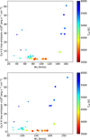 |
Fig. 6 Comparison of W0 (top) and W1 (bottom) widths and fluxes for the Ca II K emission line. The color code represents the effective temperature, and the point size represents the surface gravity, with larger points for lower gravities. |
4.3 Independence between widths and strengths of Ca II K emission line
The dependence of the WBE on gravity and effective temperature complicates the measurement of chromospheric emission since a wider bandwidth in the Ca II K line core is required with more luminous giants. In contrast, Olin Wilson’s HK Project recorded its S-index, a ratio of the combined fluxes of the Ca II emission cores, mostly only in narrow 1 Å triangular windows, divided by the flux in two symmetrically placed reference pseudo-continuum windows (see, e.g., Ayres 2019). The S-index, therefore, is insensitive to transparency fluctuations, but a color-dependent transformation into fluxes complicates its use in absolute terms (Mittag et al. 2013). In addition, for giants, experimental measurements were made in a 2 Å window, but beyond luminosity class III, even that is not wide enough. Approaches based on Mg II satellite data, on the other hand, were long limited by notorious distance uncertainties of giant stars.
Therefore, any empirical relation between the widths and spectral surface fluxes of the Ca II K emission has never been clear, if there is one at all. Our results, in units of ergs per second per square centimeter, are shown in Fig. 6 in comparison with the widths W0 and W1. The color code represents the effective temperature, and the point size represents the surface gravity (larger points for lower gravities). In fact, a straight relation between widths and fluxes is not obvious. However, it is easy to notice that there is a segregation in the K emission line flux of Ca II above ≈9 × 10⁶ erg s−1 cm−2 for the most “active” stars in our sample. Figure 7 shows the same empirical segregation on a flux-gravity dependence. The underlying physical relation could be the trend for more massive luminous giants to be more active (Schröder et al. 2018).
Dependence of the Ca II K emission line fluxes with surface gravity and effective temperature.
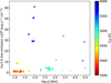 |
Fig. 7 Dependence of Ca II K emission line flux on log g. The color code represents the effective temperature, and the point size represents the surface gravity, with larger points for lower gravities. A segregation in the K emission line flux of Ca II above 10 × 106 erg s−1 cm−2 can be seen for the most “active” stars in our stellar sample. |
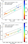 |
Fig. 8 Dependence of K emission line flux of Ca II with Teff by subtracting the gravity contribution for G1 (top) and G2 (bottom) groups. The blue line corresponds to a linear fit. The color code represents the effective temperature, and the point size represents the surface gravity – larger points are for lower gravities. |
4.4 Dependence of the Ca II K emission line flux on gravity and effective temperature
Based on Fig. 7, some involvement of surface gravity in empirical flux-temperature dependence of the Ca II K line fluxes can be suspected. Therefore, we explored empirical relations with both the main stellar parameters (i.e., surface gravity and effective temperature) and for two groups: one group including the “active” stars (G1) and another group (G2) with only the “nonactive” stars, FCa II < 9 × 10⁶ erg s−1 cm−2. We used a simple power law in the following logarithmic form:
![Mathematical equation: $\[\log~ F_{\text {Ca II }}=\alpha^{\prime} ~\log~ g+\beta^{\prime} ~\log~ T_{\text {eff }}+C^{\prime},\]$](/articles/aa/full_html/2024/12/aa50691-24/aa50691-24-eq8.png) (4)
(4)
where α′, β′, and C′ are fitting constants. Table 2 shows the results for these values when we apply Eq. (4) considering the special cases when α′ = 0 (i.e., a “pure” dependence on effective temperature) and β′ = 0 (i.e., a “pure” dependence on gravity).
Based on the results of the statistically best-matched empirical relation performed by the Kolmogorov-Smirnov test, we observed that considering a dependence on both stellar parameters (i.e., surface gravity and effective temperature) yields a better correlation than a dependence on only the effective temperature or surface gravity. However, it is clear that the main dependence of the K emission line flux of Ca II is on the effective temperature. In addition, considering the range of values of surface gravity, the dependence on this second stellar parameter does not seem to be negligible. The direct dependence of log FCa II with log Teff subtracting the respective contribution of log g for the two groups is shown in Fig. 8.
The largest α′ and β′ exponents among the G1 stars seem to be more related to the activity levels rather than to the stellar luminosity class (dwarf, giant, or supergiant). However, high temperature exponents were also observed by Ayres (2023) when analyzing the relation for the widths of the Mg II h&k emission lines with surface gravity and effective temperature.
Obviously, underlying these relations is stellar evolution in the HRD, as gravity drops strongly as a star ascends in the giant branches, while its temperature decreases by only a small amount. Ayres (2023) argues that the larger temperature exponent is possibly because there is a rough systematic shallow correlation between temperature and gravity among giants and supergiants but a steeper inverse relation among the dwarfs. Again, we believe that the tendency of more massive giants occupying larger luminosities higher up on the giant branches in part explains the empirical relations derived above in a physical way.
Data availability
The rescaled profiles of the K emission line of Ca II are available at: https://bit.ly/3VNzqMC. The flowchart of SPARTAN v1.1.3, the list of selected lines for spectral synthesis, and an example of an automatically normalized spectrum are available at: https://bit.ly/3y8cqzP.
Acknowledgements
This study used the services of the Strasbourg astronomical data center, and data from the European Space Agency (ESA) mission Gaia (https://www.cosmos.esa.int/gaia), processed by the Gaia Data Processing and Analysis Consortium (DPAC; https://www.cosmos.esa.int/web/gaia/dpac/consortium). The authors appreciate the valuable work of Sergi Blanco-Cuaresma, CfA, Harvard-Smithsonian, on ISPEC, a very useful tool for spectral analysis and parameter synthesis. This work benefited from financial support of the bilateral project CONACyT-DFG No. 278156 for the TIGRE collaboration with the University of Hamburg, and from general support of our home institutions.
Appendix A Additional tables
Distances, magnitudes, physical parameters, and parallax-based gravities.
Stellar parameters derived with the SPARTAN script.
Width and flux measurements of the K emission line of Ca II.
References
- Alvarez, R., & Plez, B. 1998, A&A, 330, 1109 [NASA ADS] [Google Scholar]
- Aurière, M., Konstantinova-Antova, R., Charbonnel, C., et al. 2015, A&A, 574, A90 [Google Scholar]
- Ayres, T. R. 1979, ApJ, 228, 509 [NASA ADS] [CrossRef] [Google Scholar]
- Ayres, T. 2023, ApJS, 266, 6 [NASA ADS] [CrossRef] [Google Scholar]
- Ayres, T. R. 2019, Stellar and Solar Chromospheres and Attendant Phenomena (Amsterdam: Elsevier), 27 [Google Scholar]
- Ayres, T. R., Linsky, J. L., & Shine, R. A. 1975, ApJ, 195, L121 [NASA ADS] [CrossRef] [Google Scholar]
- Ayres, T. R., Brown, A., & Harper, G. M. 2003, ApJ, 598, 610 [NASA ADS] [CrossRef] [Google Scholar]
- Baliunas, S. L., Donahue, R. A., Soon, W. H., et al. 1995, ApJ, 438, 269 [Google Scholar]
- Basri, G. S., & Linsky, J. L. 1979, ApJ, 234, 1023 [NASA ADS] [CrossRef] [Google Scholar]
- Blanco-Cuaresma, S. 2019, MNRAS, 486, 2075 [Google Scholar]
- Blanco-Cuaresma, S., Soubiran, C., Heiter, U., & Jofré, P. 2014a, A&A, 569, A111 [CrossRef] [EDP Sciences] [Google Scholar]
- Blanco-Cuaresma, S., Soubiran, C., Jofré, P., & Heiter, U. 2014b, A&A, 566, A98 [NASA ADS] [CrossRef] [EDP Sciences] [Google Scholar]
- Casagrande, L., & VandenBerg, D. A. 2014, MNRAS, 444, 392 [Google Scholar]
- Casagrande, L., & VandenBerg, D. A. 2018, MNRAS, 475, 5023 [Google Scholar]
- Catanzaro, G. 1997, Ap&SS, 257, 161 [NASA ADS] [CrossRef] [Google Scholar]
- Choi, J., Dotter, A., Conroy, C., et al. 2016, ApJ, 823, 102 [Google Scholar]
- Cuntz, M., Schröder, K.-P., Fawzy, D. E., & Ridden-Harper, A. R. 2021, MNRAS, 505, 274 [CrossRef] [Google Scholar]
- Dotter, A. 2016, ApJS, 222, 8 [Google Scholar]
- Duncan, D. K., Vaughan, A. H., Wilson, O. C., et al. 1991, ApJS, 76, 383 [Google Scholar]
- Eberhard, G., & Schwarzschild, K. 1913, ApJ, 38, 292 [Google Scholar]
- ESA. 1997, The Hipparcos and Tycho Catalogues (ESA SP-1200) [Google Scholar]
- Fawzy, D. E., & Cuntz, M. 2018, Ap&SS, 363, 152 [NASA ADS] [CrossRef] [Google Scholar]
- Fawzy, D. E., & Cuntz, M. 2021, MNRAS, 502, 5075 [CrossRef] [Google Scholar]
- Gaia Collaboration (Prusti, T., et al.) 2016, A&A, 595, A1 [NASA ADS] [CrossRef] [EDP Sciences] [Google Scholar]
- Gaia Collaboration (Brown, A. G. A., et al.) 2021, A&A, 649, A1 [NASA ADS] [CrossRef] [EDP Sciences] [Google Scholar]
- González-Pérez, J. N., Mittag, M., Schmitt, J. H. M. M., et al. 2022, Front. Astron. Space Sci., 9, 912546 [CrossRef] [Google Scholar]
- Grevesse, N., Asplund, M., & Sauval, A. J. 2007, Space Sci. Rev., 130, 105 [Google Scholar]
- Griffin, R. F. 2000, Ap&SS, 271, 205 [NASA ADS] [CrossRef] [Google Scholar]
- Gustafsson, B., Edvardsson, B., Eriksson, K., et al. 2008, A&A, 486, 951 [NASA ADS] [CrossRef] [EDP Sciences] [Google Scholar]
- Hauschildt, P. H., & Baron, E. 1999, J. Comput. Appl. Math., 109, 41 [NASA ADS] [CrossRef] [Google Scholar]
- Hauschildt, P., & Baron, E. 2005, Mem. Soc. Astron. It. Suppl., 7, 140 [Google Scholar]
- Hawkins, K., Jofré, P., Heiter, U., et al. 2016, A&A, 592, A70 [NASA ADS] [CrossRef] [EDP Sciences] [Google Scholar]
- Heiter, U., Jofré, P., Gustafsson, B., et al. 2015, A&A, 582, A49 [NASA ADS] [CrossRef] [EDP Sciences] [Google Scholar]
- Hubeny, I., & Mihalas, D. 2014, Theory of Stellar Atmospheres: An Introduction to Astrophysical Non-equilibrium Quantitative Spectroscopic Analysis, Princeton Series in Astrophysics (Princeton: Princeton University Press) [Google Scholar]
- Husser, T. O., Wende-von Berg, S., Dreizler, S., et al. 2013, A&A, 553, A6 [NASA ADS] [CrossRef] [EDP Sciences] [Google Scholar]
- Jofré, P., Heiter, U., Soubiran, C., et al. 2014, A&A, 564, A133 [NASA ADS] [CrossRef] [EDP Sciences] [Google Scholar]
- Jofré, P., Heiter, U., Soubiran, C., et al. 2015, A&A, 582, A81 [Google Scholar]
- Jofré, P., Heiter, U., Worley, C. C., et al. 2017, A&A, 601, A38 [Google Scholar]
- Lindegren, L., Klioner, S. A., Hernández, J., et al. 2021, A&A, 649, A2 [EDP Sciences] [Google Scholar]
- Linsky, J. L., & Ayres, T. R. 1978, ApJ, 220, 619 [NASA ADS] [CrossRef] [Google Scholar]
- Mittag, M., Schmitt, J. H. M. M., & Schröder, K. P. 2013, A&A, 549, A117 [NASA ADS] [CrossRef] [EDP Sciences] [Google Scholar]
- Mittag, M., Schröder, K. P., Hempelmann, A., González-Pérez, J. N., & Schmitt, J. H. M. M. 2016, A&A, 591, A89 [NASA ADS] [CrossRef] [EDP Sciences] [Google Scholar]
- Paxton, B., Bildsten, L., Dotter, A., et al. 2011, ApJS, 192, 3 [Google Scholar]
- Paxton, B., Cantiello, M., Arras, P., et al. 2013, ApJS, 208, 4 [Google Scholar]
- Paxton, B., Marchant, P., Schwab, J., et al. 2015, ApJS, 220, 15 [Google Scholar]
- Paxton, B., Schwab, J., Bauer, E. B., et al. 2018, ApJS, 234, 34 [NASA ADS] [CrossRef] [Google Scholar]
- Pérez Martínez, M. I., Schröder, K. P., & Hauschildt, P. 2014, MNRAS, 445, 270 [CrossRef] [Google Scholar]
- Piskunov, N. E., Kupka, F., Ryabchikova, T. A., Weiss, W. W., & Jeffery, C. S. 1995, A&AS, 112, 525 [Google Scholar]
- Plez, B. 2012, Astrophysics Source Code Library [record ascl:1205.004] [Google Scholar]
- Rosas-Portilla, F., Schröder, K. P., & Jack, D. 2022, MNRAS, 513, 906 [NASA ADS] [CrossRef] [Google Scholar]
- Ryabchikova, T., Piskunov, N., Pakhomov, Y., et al. 2016, MNRAS, 456, 1221 [CrossRef] [Google Scholar]
- Schmitt, J. H. M. M., Schröder, K. P., Rauw, G., et al. 2014, Astron. Nachr., 335, 787 [NASA ADS] [CrossRef] [Google Scholar]
- Schröder, K. P., Schmitt, J. H. M. M., Mittag, M., Gómez Trejo, V., & Jack, D. 2018, MNRAS, 480, 2137 [CrossRef] [Google Scholar]
- Schröder, K. P., Mittag, M., Flor Torres, L. M., Jack, D., & Snellen, I. 2021, MNRAS, 501, 5042 [CrossRef] [Google Scholar]
- Soubiran, C., Le Campion, J.-F., Brouillet, N., & Chemin, L. 2016, A&A, 591, A118 [NASA ADS] [CrossRef] [EDP Sciences] [Google Scholar]
- Willmer, C. N. A. 2018, ApJS, 236, 47 [Google Scholar]
- Wilson, O. C. 1978, ApJ, 226, 379 [Google Scholar]
- Wilson, O. C., & Bappu, M. K. 1957, ApJ, 125, 661 [NASA ADS] [CrossRef] [Google Scholar]
All Tables
Results for the gravity and temperature dependence of the WBE considering different measurements of the K emission line of Ca II.
Dependence of the Ca II K emission line fluxes with surface gravity and effective temperature.
All Figures
|
Fig. 1 Flowchart for determining the surface gravity log g. The term mV is the photometric apparent magnitude in the visual band, and B − V is the color index. The term V is the absolute magnitude in the visual band, BC is the bolometric correction, and L is the stellar luminosity. The term M⋆ is the stellar mass, and Teff is the effective temperature. |
| In the text | |
|
Fig. 2 Grid of evolution tracks with solar metallicity for different stellar masses in solar mass units. The color scale represents the metallicity of the star. We used MIST evolutionary tracks that were calculated with MESA. |
| In the text | |
|
Fig. 3 Effective temperature, surface gravity, and metallicity comparison between the values calculated by spectral synthesis using the SPARTAN script and the average values in the PASTEL catalog. |
| In the text | |
|
Fig. 4 Differences between the stellar parameters from GBS library and SPARTAN script. The mean values and standard deviations of the differences are ΔTeff = 28 ± 70 K, Δ log g = 0.04 ± 0.09 dex, and Δ[Fe/H] = −0.01 ± 0.08 dex. |
| In the text | |
|
Fig. 5 Comparison of the synthetic stellar spectra calculated with PHOENIX for HD 124807 (Arcturus) in LTE and NLTE modes for two different wavelength regions: the Ca II K line (top) and H α line (bottom). The spectrum observed with TIGRE-HEROS has been rescaled to convert the relative intensity into physical flux given by the PHOENIX spectra. |
| In the text | |
|
Fig. 6 Comparison of W0 (top) and W1 (bottom) widths and fluxes for the Ca II K emission line. The color code represents the effective temperature, and the point size represents the surface gravity, with larger points for lower gravities. |
| In the text | |
|
Fig. 7 Dependence of Ca II K emission line flux on log g. The color code represents the effective temperature, and the point size represents the surface gravity, with larger points for lower gravities. A segregation in the K emission line flux of Ca II above 10 × 106 erg s−1 cm−2 can be seen for the most “active” stars in our stellar sample. |
| In the text | |
|
Fig. 8 Dependence of K emission line flux of Ca II with Teff by subtracting the gravity contribution for G1 (top) and G2 (bottom) groups. The blue line corresponds to a linear fit. The color code represents the effective temperature, and the point size represents the surface gravity – larger points are for lower gravities. |
| In the text | |
Current usage metrics show cumulative count of Article Views (full-text article views including HTML views, PDF and ePub downloads, according to the available data) and Abstracts Views on Vision4Press platform.
Data correspond to usage on the plateform after 2015. The current usage metrics is available 48-96 hours after online publication and is updated daily on week days.
Initial download of the metrics may take a while.