| Issue |
A&A
Volume 674, June 2023
|
|
|---|---|---|
| Article Number | A162 | |
| Number of page(s) | 10 | |
| Section | Stellar atmospheres | |
| DOI | https://doi.org/10.1051/0004-6361/202245241 | |
| Published online | 19 June 2023 | |
Discovery of an extended G giant chromosphere in the 2019 eclipse of γ Per
1
Sterrewacht Leiden,
Niels Bohrweg 2,
NL-2333CA
Leiden, Netherlands
e-mail: diamant@strw.leidenuniv.nl
2
Departamento de Astronomía, Universidad de Guanajuato,
Callejón de Jalisco s/n Col. Valenciana,
Guanajuato
36023, Mexico
3
Department of Space, Earth and Environment, Astronomy and Plasma Physics, Onsala Space Observatory, Chalmers University of Technology,
439 92
Onsala, Sweden
4
Hamburger Sternwarte, Universität Hamburg,
Gojenbergsweg 112,
21029
Hamburg, Germany
Received:
18
October
2022
Accepted:
25
March
2023
The November 2019 eclipse of γ Per was a rare opportunity to seek evidence for a chromosphere of the G8 giant, hitherto suspected but not detected. Twenty-nine years after the only other observed eclipse, we aim to find chromospheric absorption in the strong Ca II H&K lines, and to determine its column densities and scale height. Using the Telescopio Internacional de Guanajuato Robótico-Espectroscópico (TIGRE) in Guanajuato (central Mexico) before, during and after the 8 days of total eclipse, we obtained good S/N spectra of the G8 giant alone and composite spectra of the partial phases, near eclipse and far from eclipse. In the near UV of the Ca II H&K and Hϵ lines, the G giant spectrum that was adequately scaled was subtracted from the composite spectra in partial phases, near and far from eclipse, to obtain the A3 companion spectra with and without traces of chromospheric absorption. In addition, we used PHOENIX full non-local thermodynamic equilibrium model atmospheres on the blue A star spectrum, iSpec spectral analysis of the red G giant spectrum, and evolution tracks to study both components of γ Per. For the first time, we present evidence for this rare type of a not very extended G giant chromosphere, reaching out about half of an A-star radius (~1.5 Gm) with a scale height of only 0.17 Gm. By its location in the Hertzsprung-Russell diagram, the γ Per G8 giant is very close to the onset of more extended chromospheres. Furthermore, we show that this giant has a rather inactive chromosphere, and a recent 5 ksec XMM pointing reveals only a very faint, low-energy corona. While the γ Per primary has a mass of ~3.6 M⊙, and its A3 companion has one of ~2.4 M⊙, the latter is too cool (8400 ± 300 K), which is too evolved on the main sequence to be the same age as the primary. The high eccentricity of the 5329.08 days long-period orbit may therefore be reminiscent of a rare capture event. Using the eclipse method, we resolve a pivotal case of a G giant chromosphere, which seems to represent a low-gravity analogue of the inactive Sun. A systematic change of giant chromospheric extent by Hertzsprung-Russell diagram position is confirmed. Compared to the solar chromosphere, the density scale height increases with gravity by ∝ ɡ−1.5.
Key words: stars: chromospheres / binaries: eclipsing / supergiants / binaries: spectroscopic
© The Authors 2023
 Open Access article, published by EDP Sciences, under the terms of the Creative Commons Attribution License (https://creativecommons.org/licenses/by/4.0), which permits unrestricted use, distribution, and reproduction in any medium, provided the original work is properly cited.
This article is published in open access under the Subscribe to Open model. Subscribe to A&A to support open access publication.
1 Introduction
The solar chromosphere, mediating between the very different physical conditions of the photosphere and the corona of the Sun, is the only example of its kind, which can be very well resolved by imaging it in the light of its emission lines. A lot of the magnetic fine structure with supersonic dynamics dominates the upper chromosphere, notably spicules (Budnik et al. 1998, Judge & Carlsson 2010), while the denser lower chromosphere forms a thin layer of only o(2”) or o(1000) km, with a density scale height of about 100 km. For more details, readers can refer to the total hydrogen density in Fig. 5 of the model of Vernazza et al. (1973) in the height range of 200–800 km.
However, when it comes to giant chromospheres and how they differ from solar-type chromospheres, our knowledge is mainly based on indirect evidence. The classic Wilson-Bappu effect is well known (Wilson & Vainu Bappu 1957) and, at face value, states an empirical relation between luminosity and chro-mospheric Ca II K emission line width. Its interpretation as a line density broadening effect by Ayres et al. (1975) shows that despite the presence of the magnetic fine structure, the general physical conditions near the base of the chromosphere can be derived in a reasonable approximation simply from hydrostatic equilibrium in the temperature minimum with the mass column density above, in addition to it being possible to derive that the continuum opacity there (mostly produced by H− opacity) is proportional to the column density squared ( ).
).
In consequence of this approach of Ayres et al. (1975), column densities N grow with falling gravity ɡ as  . On the other hand, densities n at the base of the chromospheres with n ≈ N/Hd, keep their proportionality with gravity. Consequently, this simple description implies the density scale height Hd grows significantly towards lower gravity, with hd ∝ ɡ−1.5.
In fact, the description of Ayres et al. (1975) reproduces the Wilson–Bappu effect sufficiently well by the observed strong, primary dependence of the chromospheric Ca II K emission line width on gravity (empirically seen by the luminosity dependence), and it even explains the secondary dependence on effective temperature Teff. Qualitatively, it is an ionization effect on the Ca II column density given that the cooler giants have a noticeably larger fraction of Ca I in their chromospheres (see Rosas-Portilla et al. 2022 and discussion therein). The verified reality of the Wilson–Bappu effect, however, is more indirect evidence. Using the strong dependence of density scale height on gravity, information from resolved giant chromospheres could manage to test simple chromospheric physics.
Other important observational evidence of cool giants’ outer atmospheres is the X-ray detections across the Hertzsprung-Russell diagram (HRD). Initially, not going deep, these suggested a bifurcation into coronal and non-coronal cases (Linsky & Haisch 1979). It seemed at first those luminous cool giants had no coronal matter but cool winds instead. Subsequently including deeper detections and larger samples, however, it soon became clear that more active cool giants could have both cool winds and coronal emission at the same time (dubbed ‘hybrid stars’, see Reimers 1982), and that there is no strict division of this kind in the HRD. However, considering only giants of a low activity degree, the concept of a ‘coronal’ or ‘Linsky-Haisch’ dividing line still seems to remain true to some extent.
According to Ayres et al. (2003), there is a simple geometrical effect at work in cool giants. Coronal magnetic loops of such stars become buried under those with much larger density scale heights and column densities. In this sense, stemming from (i) the Wilson–Bappu effect and (ii) the uneven distribution of X-ray detections in the HRD, the expectations of significantly more extended chromospheres for luminous cool giants of low gravity are consistent.
In addition, Schröder et al. (2018) give reasons based on the energy balance near the ‘Athay point’. This states the boundary of the chromosphere with the corona triggered by the collapse of the neutral hydrogen reservoir and its radiative cooling (see Athay 1981). In inactive giant chromospheres, the height of the Athay point should therefore simply grow with smaller gravity and lower effective temperature, because fewer mechanical energy input meets larger column densities until complete hydrogen ionisation becomes impossible and coronae cease to exist. Only extraordinary magnetic heating would allow for high-temperature plasma within the upper chromosphere and cool wind (in the case of a hybrid star). Again, this is only circumstantial evidence for the appearance of a giant chromosphere.
Consequently, any direct observational evidence for the extent of giant chromospheres, especially in cases located in the HRD near the Linsky–Haisch dividing line, would be most illuminating and help our understanding of the basic physics of the lower chromosphere. Fortunately, such a direct observational approach is given to us using eclipsing binary stars with a giant primary. As the main sequence companion star is hotter and much smaller, it acts as a light probe to shine through the extended giant chromosphere from behind before and after the main eclipse. According to the well-observed proto-type, these binaries are called ζ Aurigae systems. Only a hand full of such precious systems have been well observed. For more details, readers can refer to Ake & Griffin (2015) and the vast literature cited therein.
The most prominent representatives of this exclusive club have K supergiant primaries (ζ Aur itself, 31 Cyg, and 32 Cyg). However, a few binaries involve a G giant, such as τ Per, HR 6902, HR 2554, and 22 Vul. Further details can be retrieved from Schröder (1990) and Schröder & Hünsch (1994). Since tau Per and HR 2554 eclipses remain partial in their maximum degree, so far only two G giant chromospheres have been well studied with the eclipse method, HR 6902 and 22 Vul.
Compared to the hugely extended K giant chromospheres, these G giants show much less extended chromospheres. However, more such case studies are required as we suspect the existence of some systematic relation with, for example, the HRD position. And we can here take advantage of their geometrically limited chromospheric nature. These G giants, γ Per in particular, should provide a good direct test to the expected relation between density scale height and gravity, as well as to the height of their Athay points.
For these reasons, γ Per with its G giant is now a very interesting candidate for providing another rare case study. However, during its first-ever observed eclipse in 1990, no chromospheric absorption could be detected (further details are available in Griffin et al. 1994). For a period of 14.5 yr, the following eclipse was unobservable in the day sky. Hence, the November 2019 eclipse presents the first chance to try again.
2 The November 2019 eclipse of γ Per
Maury & Pickering (1897) and Campbell (1908) discovered the binary nature of the γ Per system and McLaughlin (1948) determined its long orbital period of 14.6 yr from radial velocity measurements of the primary star. However, the existence of total eclipses were not discovered until 1990 by Griffin et al. (1994). In that work, observers were based on three continents with very different time zones (Europe, Japan, USA), which allowed for good coverage of the short partial phases. The good distribution of observers around the world helped to pin down the partial eclipse phases and contact points. Furthermore, the use of photometers with filters well-calibrated to the Johnson UBV system helped to establish the photometric properties of the eclipse.
2.1 Photometric observations and eclipse geometry
In 2019, two orbital revolutions later, less complete coverage with secondary calibration of the photometry (using DSLR CMOS camera photometry) onto the 1990 eclipse light curve was therefore sufficient to establish very precisely the system period of 5329.0 ± 0.05 days. This is fully consistent with the period obtained from the less time-sensitive radial velocity data. Apart from photometry by observers Wolfgang Vollman (AAVSO), based in Vienna, Austria, and Faiber Rosas–Portilla, based in Guanajuato, Mexico – shown in Fig. 1 by diagonal crosses – we were able to use the spectrophotometric estimates of partial eclipse progress from TIGRE spectra. These values were obtained in very relevant phases and projected onto the Johnson colour scale of the 1990 photometric eclipse data. The spectrophotometric estimates are depicted in Fig. 1 by the small vertical bars from above. A best-fit superposition of our 2019 eclipse photometry onto the 1990 eclipse light curve in the Johnson B filter is shown in Fig. 1. The eclipse depths in B, due to the blue colour of the eclipsed companion, are considerably deeper than the V light curve, but less sensitive to atmospheric transparency problems than in U, and so presents the best means to time the eclipse.
According to the good quality Johnson photometry of the 1990 eclipse presented by Griffin et al. (1994), the eclipse depths are 0.54 mag in B and 0.28 mag in V while the system’s total brightness of B = 3.63 and V = 2.93 mag. This suggests individual brightnesses and colours of the G giant of V = 3.21 and B – V = +0.96 mag and of the A star companion of V = 4.54 and B – V = +0.11 mag. As the distance to γ Per is rather small (71 pc according to GAIA EDR3 parallax) and in that galactic longitude, we assume that the interstellar reddening is negligible.
Mid-partial eclipse phases set the zero points of the height scales on either side to JD 2458 804.8 and −814.0 (±0.1d), respectively. This yields an eclipse radius of the giant of 22.7 R⊙.
A central eclipse path may be assumed since this giant eclipse radius agrees well with the luminosity radius derived from the GAIA EDR3 parallax (14.12 mas, and see Sect. 5).
Interestingly, TESS photometry (publicly available now) covered the first three eclipse contacts. It shows an eclipse depth of only 0.14 mag but a quantitative interpretation of these data is difficult due to possible saturation effects and the filter response function differs from Johnson V. Nonetheless, the TESS light-curve is of a very high cadence and therefore resolved those first three contact points relatively well. Using these to verify our above photometric results, we find very good agreement within the stated uncertainties. In particular, TESS ingress data set mid-partial eclipse at JD 2458 804.8, too, and give a partial eclipse duration of 1.60 (±0.05) days. Totality lasted 7.4 (±0.05) days, mid-totality fell on JD 2458 809.3.
With the zero points of the projected height scale on either side of the eclipse now well-timed, all we need is the tangential velocity to define the projected heights at the times our spectra were taken (see Table 1 and next section). As suggested by Griffin et al. (1994), we use a constant value of 40.0 km s−1 as an approximation which is based on the spectroscopic orbit and a mass ratio of (or near to) 1.5. The latter is also consistent with the masses of our evolution tracks which match the HRD positions of both components. For further details, readers can refer to Sect. 4.
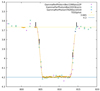 |
Fig. 1 Merged eclipse light curve in the Johnson B filter of the 1990 (see + symbols of “GammaPerPhotomBecl1990plus2P” dataset) and 2019 photometry (see x symbols of “GammaPerPhotomBecl2019norm” dataset) on the 2019 JD scale (add 2458000 to x-axis values), by applying a best-fit period of 5329.08 days. TESS 2019 photometry is added, as well as spectrophotometry by TIGRE (“GammaPerPhotomTI-GREecl2019” data), and all 2019 data are scaled to the Johnson B eclipse depth of 1990. |
2.2 Spectroscopic observations with TIGRE
Table 1 lists the TIGRE spectra obtained before, during and after the 2019 eclipse of γ Per. The TIGRE’s fibre-fed HEROS spectrograph is placed on a massive bench in an air-conditioned annex beside the dome. Its performance as well as the most relevant technical details have been described by Schmitt et al. (2014). With respect to the observations used for this work and in the context of relative spectrophotometry (refer to Sect. 3.1), we like to add that the fibre entrance projected on the sky measured 3 arcsecs. Usually, the apparent seeing disk of the star including short-term impact on the pointing by wind and guiding errors is of the order of 2 arcsecs or better. The nights of spectroscopy used for γ Per were all of the regular quality in that respect. Using ample exposure times for such a bright star (4 min), we obtained a very good and uniform S/N in the here listed blue spectra in partial and chromospheric eclipse and the pure G giant spectra from a total eclipse of 100–120.
The projected heights of the centre of the A star above (or under, when negative) the G giant limb are listed in the second-last column. Total eclipse spectra provided a reference to the pure G giant spectrum. Subtracting this from the composite spectrum left us with the pure A star companion spectrum, which gave us the estimate of partial eclipse depth. This finding agrees with the photometric data and resulting eclipse timing. During and just outside the partial eclipse, we also found traces of chromospheric Ca II H&K line absorption. Further details are stated below.
However, in this case of a geometrically much less extended G giant chromosphere, there is a complication. The companion star here is a lot larger than the chromospheric density scale height. When light is simultaneously passing chromospheric layers of very different column densities, any quantitative interpretation of the chromospheric Ca II line absorption in the spectrum of the companion shining from behind here requires a detailed consideration of how the absorption line profile is formed. We here take the approach shown by Schröder et al. (1996), then used on the chromosphere of HR 6902. Based on that study, the last column in Table 1 gives an ‘effective height’ of the not eclipsed A star disk at that moment, halfway between the projected outer edge of the A star and the giant photosphere,  .
.
Information about the date and time of the eclipse data of Gamma Persei.
3 Dissecting the composite spectrum
Compared to what was available during the previous eclipse observations in 1990, we subsequently demonstrate in this publication that better phase timing and high signal-to-noise (S/N) detectors allowed us to finally detect and quantify the chromo-spheric line absorption in the light of the A star companion beyond doubt. A subtraction technique was used which is similar to how the classical zeta Aur systems were studied (see, e.g. Griffin et al. 1990). The pure G giant total eclipse spectrum was employed to reduce the composite spectra to the A star spectrum and any traces of the chromosphere in front of it.
The subtraction has to be done very carefully by the right proportions in the composite spectrum because Popper & McAllster (1987) reported that the Ca II K line appears in both the companion star and giant in the γ Per spectra. Owing to the high abundance of Ca II ions in the chromosphere, the H&K absorption lines of the Ca II ion are usually the first absorption features in chromospheric eclipse spectra. Considering that the Ca II H line is blended with Hϵ, we only used the K line at 3933.66 Å and its profile for our analysis of the chromospheric absorption. As large column densities cause strong core saturation, the Lorentz damping wings become a sensitive element in the density analysis (see, e.g. Schröder et al. 1994). Probed at several projected heights, the extent and density scale height of the chromosphere can be determined. We lay out this subject in more detail below. However, it is necessary to first extract the chromospheric absorption from the Ca II K line. This is imprinted on the A-star companion spectrum from the composite spectra in the blue and near UV.
3.1 Scaling and subtracting the pure G giant spectrum
For a consistent spectrophotometric approach, we did not use continuum-normalized TIGRE spectra, but a version which is calibrated relative to the physical flux of a standard A star. Then to obtain the Ca II К line chromospheric absorption, the main step was to subtract the total eclipse G giant spectrum (in Table 1 listed as 18.11.2019) in the right flux proportions from each of the composite spectra obtained for this study.
For the practical implementation of the spectral subtraction process, we used the spectroscopic analysis and graphics software package iSpec in its latest Python 3 version (v2020.10.01), (Blanco-Cuaresma 2019). The spectrum relatively far outside the eclipse (in Table 1 listed as 28.11.2019) gives a good illustration of the steps taken here (see Sects. 3.1–3.3) and its result serves as a reference to the sole A-star spectrum. The same procedure was applied to the other spectra listed in Table 1 except that the two partial eclipse phases required a different scaling of the flux ratio between the giant and the A-star. In the first step, all spectra were corrected for the radial velocity to the rest frame of the G giant.
Our spectrophotometry is only of a relative nature given the standard stars could not be taken at the exact same airmass and time. However, there is still an advantage in using fluxes normalized to the physical flux of our A0-type standard stars. In practical terms, it means that any slopes across the spectral range of interest are physical and not instrumental in nature. Differences in the absolute scale were accounted for by an empirical scaling of the G giant spectrum from total eclipse. To be subtracted in the right proportion, we analysed the residuals of the lines present in the G giant spectrum over a series of subtractions with a slightly varied scaling factor. When not enough G giant is subtracted, its photospheric lines remain visible in the result and when it is too much, the G giant spectral features go into reversal. Fortunately, in the case of γ Per there are many small photospheric G giant lines without any chromospheric absorption component. Furthermore, we found enough consistency in this approach to calibrate the respective flux scaling factors to better than 5% which is also the small order of uncertainty of the Ca II H&K line profiles of the subtracted spectra.
Obviously, we focussed this effort on the Ca II H&K region. The two Balmer lines here in the A-star spectrum have broad wings and their shallow slopes need to be extracted in a realistic way which serves as an additional criterion to determine the best-fitting scale factor for the subtraction (as shown in Fig. 2).
These subtraction results now contain the chromospheric density information in the form of the Ca II line absorption imprinted on the A-star companion spectrum in different degrees. It depends on the proximity to the eclipse as shown in Fig. 3.
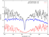 |
Fig. 2 Flux-calibrated spectra of the composite spectrum from a phase outside eclipse (28 November 2019, black), G giant only in total eclipse (red) and subtraction to gain pure A star spectrum (blue), around the Ca II K line (3933 Å), which sees contributions from both stars. |
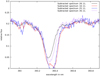 |
Fig. 3 Subtracted spectra (A-star only) from outside eclipse (28 November 2019, black), chromospheric eclipse ingress (16. Nov. 2019, red), partial and chromospheric eclipse egress (25 November 2019, blue) and chromospheric egress (26 November 2019, purple), focussed on the Ca II K line. |
3.2 A useful byproduct: analysing the disentangled companion A star spectrum
In a final step to quantify the chromospheric line absorption, the subtracted spectra must be normalized by dividing each one by the exact pure A star spectrum, at the right radial velocity offset of the latter from the G giant. For this, we used the one obtained from the subtraction of the 28 November 2019 spectrum which was taken far outside the eclipse. Here, the crucial point is the relatively (compared to other early type A stars) slow rotation of the γ Per A star companion, and the fact that it has a notable Ca II K line of its own. The use of a template A star spectrum risks mismatching the latter in width and depth a bit by not finding the exact right rotation velocity. Hence, the only solution is to use a spectrum of the original star, and so to accept its larger noise, stemming from the subtraction.
However, as we were also concerned about its spectropho-tometric reliability, we first compared the extracted companion A star spectrum with synthetic spectra and their spectral surface fluxes. The latter spectra were computed with PHOENIX full non-local thermodynamic equilibrium (NLTE) model atmospheres for a variety of effective temperatures. For more details, readers can refer to Hauschildt & Baron (1999). Figure 4 shows the best-matching PHOENIX model (blue) of an effective temperature of 8500 K together with our subtracted spectrum of the γ Per companion of 28 November 2019 (red).
Our effective temperature value agrees very well with earlier empirical work on the A star companion because Popper & McAlister (1987) quantified it as 8318 K. As for metallicity, we used [Fe/H] = −0.2, as suggested by citet McWilliam 1990, and we adopted a best-matching rotational broadening of 40 km s−1. The resulting PHOENIX model with 8350 K and log ɡ = 3.5 (as of a late main-sequence star, see below and Table 2) is a very good match to the Balmer Hϵ line which is blended with the Ca II H line around 3967 Å. As a byproduct, this revised effective temperature of the companion is of significance to our understanding of the binary and its formation history as we further discuss below.
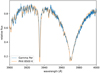 |
Fig. 4 Ca II H&K and Hϵ region of the sole A star spectrum (blue) obtained from the subtraction of the out-of-eclipse spectrum of 28 November 2019 matched by a complete NLTE PHOENIX model spectrum for 8500 K (red), log ɡ = 3.5 and [Fe/H] = −0.2. |
3.3 The chromospheric extent, as revealed by the subtraction method
Before attempting a quantitative chromospheric absorption line profile analysis, we performed direct comparisons of the subtracted spectra with the one of the pure A star far outside the eclipse. This demonstrates the presence of chromospheric absorption in the Ca II K line (see Fig. 3), and to see how far out it can be traced.
These figures reveal a substantial amount of red-shifted chro-mospheric absorption, thereby proving it to be in the rest frame of the giant. Note, this orbit is highly eccentric (0.785, Pourbaix 1999) and therefore the radial velocities of companion and primary differ around the eclipse. The chromospheric extent can be determined using the A-star’s projected height, or in the different partial eclipse spectra, by the effective height of its not eclipsed disk (see Table 1).
At ingress, during the partial eclipse of 16 November 2019, a half occulted A star reveals a very strong chromospheric Ca II K line absorption in the line of sight to its outer half (see again Fig. 3). During the 25 November 2019 spectrum at egress, about two-thirds of the companion star is still occulted by the giant and the not eclipsed third suffers a highly saturated amount of chromospheric Ca II K line absorption. About 24 h later, it decreases considerably to only a partial absorption in the line core. Now, two-thirds of the A-star disk is out from the G giants occultation and its outermost area may already be free from any Ca II K line absorption. Therefore, a conservative estimate of the chromospheric extent amounts to one A star radius or 3.9 R⊙ (see Griffin et al. 1994, Popper & McAlister 1987 and above).
Summary of the physical parameters of the γ Per components derived in this work, see text for more information.
3.4 Chromospheric absorption line profile modelling
During the eclipse by a geometrically thin chromosphere, strongly stratified Ca II layers of very different densities are seen against the disk of the companion which in some cases (e.g. HR 6902 and γ Per) is much larger than the density scale height of the chromosphere. This is quite different from the situation in the classical ζ Aur systems with K supergiants and their hugely extended chromospheres where the companion stars can safely be treated as point light sources.
For HR 6902, Schröder et al. (1996) already modelled pure line absorption in the presence of a steep chromospheric density gradient, showing that even a single Ca II K chromospheric absorption line profile holds essential clues to the density scale height across the companion stars disk. We here used the same method, which is described in detail by Schröder et al. (1996). The Fortran programme was updated only with respect to the TIGRE-HEROS spectrograph line profile broadening and the eclipse geometry of γ Per, that is, its secondary radius. Modelled pure chromospheric absorption line profiles are matched to the subtracted spectra presented above, after dividing the latter by the pure A star spectrum (matching the A star radial velocity rest frame in each case). This is done in order to normalize the observed chromospheric absorption to the exact underlying spectrum. We note that by this, division noise is amplified in the core of the A star’s Ca II K line which falls to the blue side of the deepest chromospheric absorption.
Figures 5–7 display the best-matching Ca II K line absorption models (dashed line) applied to the observed chromospheric absorption (solid line), extracted as described above for the phases listed in Table 1. Furthermore, Table 3 lists the derived values of the apparent turbulence velocity (υturb), column density (N) at the effective height of the companion star and the scale height (α) of the chromospheric density distribution in front of it, together with the respective projected ( ) and effective heights (
 ) (see Sect. 2).
Compared to simple point source absorption, these Ca II K line profile models shown here appear rather broad for their modest degree of saturation. This is the effect of mixing contributions from lines of sight with very different column densities, some leading to strong saturation while others are optically thin. Otherwise, extreme supersonic (about 35 km s−1) line broadening would be required. Still, with a steep density gradient and a scale height as small as 0.17 GM, we require apparently supersonic turbulence of 18 and 14 km s−1 to match the observed profile. Similar turbulent broadening velocities were found for the chromosphere of HR 6902 by Schröder et al. (1996). Since on a small scale, supersonic motions would quickly be damped away, this result hints at macroscopic entities which move with such speeds through the chromosphere and are adding up to contribute a large part of the absorption detected. A plausible explanation is spicules, in the solar case their supersonic motions are well documented (see, e.g. Judge & Carlsson 2010).
Regarding the chromosphere’s symmetry, we compare the column densities found in ingress and egress by plotting them over their respective ‘effective heights’ in Fig. 8. It may be concluded that the chromosphere is almost symmetric, yet there is some local variation which again plausibly hints at an irregular carpet of spicular-like features.
Furthermore, the steep decline of the four individual column densities over effective height translates into a small density scale height of o(0.2GM) throughout the chromosphere, confirming the result (see Table 3) from individual absorption line profile modelling for the lower layers. Such information and the well-defined limited extent of this giant chromosphere, raise the question if this can be a case of a low-gravity solar analogue.
For that matter, we compare the chromospheric density scale height of γ Per (0.17 Gm) to that of the lower part of the solar chromosphere (about 100 km, according to the model of Vernazza et al. 1973). We may here assume that Ca II represents total chromospheric densities sufficiently well in both cases, given similar temperatures (4970 K, see below and Table 2, versus 5775 K, or 0.06 dex). Any effect on the chromospheric scale heights Hd could only be of a secondary nature. The one of the giant is larger than the solar by a factor of about 1700 or 3.23 dex, while its gravity is lower by 4.44 − 2.23 = 2.21 dex (see the gravity of γ Per derived below). As described in the introduction, the successful approach of Ayres et al. (1975) to explain the Wilson Bappu effect implies a relation of Hd ∝ ɡ−1.5 which is in total agreement with our result, within the observational uncertainties.
Results from the line absorption modelling applied to the Ca II K line of the γ Per giant.
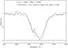 |
Fig. 5 Line absorption model (dashed line) applied to the giant’s chromospheric absorption (solid line) of the Ca II K line on the 16 November 2019 subtracted spectrum in ingress, normalized to the pure A star spectrum. |
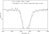 |
Fig. 6 Line absorption model (dashed line) applied to the giant’s chromospheric absorption (solid line) of the Ca II K line on the 25.11.2019 subtracted and normalized spectrum in egress, still in partial eclipse. |
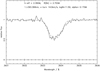 |
Fig. 7 Line absorption model (dashed line) applied to the giant’s chromospheric absorption (solid line) of the Ca II K line on the 26.11.2019 subtracted and normalized spectrum in egress. |
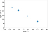 |
Fig. 8 Column density vs. effective height from line absorption modelling with the estimated uncertainties of 0.5 dex in N and 0.1 Gm in height. See Table 3 for data. |
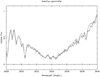 |
Fig. 9 Comparison of the Ca II K line cores of the low activity Hyades early K-type giant ϵ Tau with the γ Per late G giant shows nearly perfect coincidence, demonstrating the low-activity nature of the latter despite its larger mass. While these spectra are virtually identical inside the Ca II K line, the gamma Per G giant’s spectrum contains the most noise. |
4 The low activity of both chromosphere and corona of γ Per
As obtained during the total eclipse, the Ca II K emission of γ Per giant compares very well with that of the low-activity early K-type giant ϵ Tau of the near Hyades cluster (see Fig. 9). The latter is less massive (2.7 M⊙) and less luminous. Consequently, in the HRD ϵ Tau has a similar proximity to the inclined “Mg II dividing line” as γ Per despite its slightly later spectral type.
This low degree of activity is also confirmed by a recent detection (Sept. 11, 2022) of a faint, low-energy corona of γ Per by a 5 ks pointing with XMM (see Fig. 10). It confirms that a 1990’s ROSAT detection, with an offset of 45 arcsec from γ Per, is indeed a separate source. Within 15 arcsec around the position of the star, there is a statistically significant detection in the band of OVIJ (of low energy, around 0.58 keV) of 7 photons above the background of 3 photons, but remains insignificant in the other bands of XMM. This observation translates into a very low and soft X-ray coronal surface flux of Fx = 50 erg cm−2 s.
Even if part of this coronal emission remains unaccounted for by blending with the background, Fx of γ Per thus is two orders of magnitude lower than the minimal flux (≈ 104 erg cm−2 s) of inactive main sequence stars reported by Schmitt (1997). Additionally, it is still fainter by one order of magnitude than the Fx of ϵ Tau (see Schröder et al. 2020 and references therein), which is consistent with the proximity to the coronal dividing line of both these giants.
Hence, we may conclude that the geometrical properties of the chromosphere of γ Per reported above are not disturbed by any local magnetic fields and indeed represent a low-gravity analogue of the solar chromosphere outside active regions.
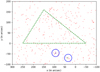 |
Fig. 10 Soft X-ray photons detected by an 5 ksec XMM pointing in the OVΠ band (0.425–0.725 keV) at the position of γ Per (upper left circle) exceed the background count of 3 by statistically significant 7 extra photons. The lower right circle shows a separate, much harder source already detected by a 1990s pointing of ROSAT. The green striped triangle area is the source-free reference field which is used to determine the background. |
5 The γ Per G giant in the Hertzsprung–Russell diagram
5.1 A phenomenological comparison
In order to explore the relation between chromospheric properties of γ Per and related G giants in eclipsing binaries and their positions in the HRD, for simplicity, we first compare these candidates in the observational HRD, that is by their absolute visual magnitudes MV and В – V colours. For γ Per, the eclipse photometry (see Sect. 2) yields a G giant colour of В – V = 0.96 and with the GAIA EDR3 parallax of 14.12 ± 0.77 mas, a distance modulus of M – m = 4.25mag is obtained. With В – V = 3.21 for the γ Per G giant alone (see again Sect. 2), its absolute visual magnitude is then MV = −1.04.
For τ Per, HR 6902, HR 2554, and 22 Vul we use the same values as adopted by Schröder (1990) in their Fig. 3 and used by Griffin et al. (1992). Those graphs served a similar purpose at the time, which is to compare the giant positions in the observational HRD to the classical ‘dividing lines’ (see Fig. 11). While it is long clear that there is not a strict division between coronae and cool winds, however, the vertical distance from these lines seems to be related to the chromospheric density scale heights and extent found by us and seems to relate to the vanishing of coronal emission in low activity giants. The specific dividing lines depicted here were originally from Mullan & Stencel (1982) and we refer to the original literature for more detail.
In particular, we note that HR 6902 compares well to γ Per. Both these giants undergo full eclipses (see Griffin & Griffin 1986) and have a geometrically rather modest chromosphere, detected out to 0.1 RG (= 3.3 R⊙). But the chromospheric absorption of HR 6902 appears to be denser at its bottom when compared closely with gamma Per. The chromospheric density scale height of HR 6902 was found (Schröder et al. 1996) to be 0.3–0.6 GM, this is small compared to the classical ζ Aur chromospheres, but larger than in γ Per. Further outside of the HR 6902 eclipse, the presence of geometrically extended plasma of transition region temperature (o(200 000) K) was revealed by С IV and Si IV line absorption (Kirsch et al. 2001, Ake 2002). Both G giants have a similar position in the HRD relative to the domain of coronal and non-coronal giants, but HR 6902 is a bit closer to the cool giants’ side.
Additionally, HR 2554 shows signatures of Si IV and СIV line absorption. It is a minor X-ray detection by ROSAT, which suggests that coronal and transition region plasma seem to coexist in these transitional late G giants, in terms of some kind of X-ray-faint hybrid corona. In the observational HRD, like γ Per, HR 2554 lies rather close to the coronal side (see Fig. 11).
Unfortunately, HR 2554 undergoes only grazing eclipses, which means that its chromospheric line absorption evidence is less solid. Eclipse observations of Schröder & Hünsch (1992) from 1990 suggest a very small chromospheric extent of only 0.3 R⊙, and this find may simply be reflecting the procedural disadvantage of dealing with a partial eclipse, which does not allow a very exact spectral subtraction.
In summary, the γ Per giant chromosphere has the smallest density scale height among all ζ Aur type binaries with total eclipses, while being the closest of all these giants towards the coronal side of the HRD. It seems to be a low-gravity inactive solar analogue and an ideal test case for chromospheric physics. Unfortunately, γ Per has not yet been probed for СIV and Si IV line absorption, which would complement its faint soft X-ray detection presented above.
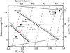 |
Fig. 11 Positions of the giants in ζ Aurigae, 31 Cygni, 32 Cygni, 22 Vul, HR2554, HR6902 and τ Per, as well as of γ Per (red dot) in the observational HRD, in comparison with the ‘dividing lines’ between coronal (left) and cool wind (right) type stars, adopted from Schröder (1990) and Griffin et al. (1992). |
5.2 Spectral synthesis of physical parameters and evolution models
In order to make a quantitative analysis of the interesting γ Per binary system, exact effective temperatures and luminosities of both stars are required to compare with well-tested evolution tracks. We use the code and parameterization detailed by Pols et al. (1998) and Schröder et al. (1997).
For the G giant, we attempted to determine the effective temperature with the spectral synthesizing tool iSpec (Blanco-Cuaresma 2019) using a good S/N red channel TIGRE spectrum from the 2019 total eclipse. As pointed out by Schröder et al. (2020), solutions are not unique and cross-talk between parameters leads to different parameter combinations with almost the same minimal residuals.
Therefore, we used the approach of Schröder et al. (2020) by prefixing gravity from available non-spectroscopic information (here namely the eclipse radius of 22.7 R⊙ from Sect. 2, and the mass estimate, see below), and we obtained log ɡ = 2.23. We also used the same line list, well-tested for G-type main-sequence stars. The lowest residuals are then pointing to a solution of 4931 K and an enhanced metallicity of [Fe/H] = 0.32, however, with an estimated systemic uncertainty of about 70 K. Then, as an alternative approach, we tried a larger line list, newly derived and successfully tested for K giants by us (Rosas-Portilla et al. 2022, for technical details, see appendix therein). That approach yields the lowest residuals solution for 5032 K and a lower metallicity of −0.16, giving a matching gravity of log ɡ = 2.3 without the need to prefix it.
As both results suffer from similar systemic uncertainties and the G giant is right in between the two different parameter regimes for which each line list works best, we here adopt 4970 K and a solar abundance. This is in good agreement with the spectral type of G9 III and the primary star’s genuine colour of В – V = 0.96. The latter leads to a bolometric correction of ВС = −0.34 (using Flower 1996, Table 3), with which we obtain MBol = −1.38, or log L = 2.45 L⊙ (using MBol⊙ = 4.74). This is fully consistent with the eclipse radius (22.7 R⊙), giving the same luminosity with the here adopted value of Teff.
For the A star companion, eclipse photometry (B and V depths of totality in particular, see Sect. 2) yields individual brightnesses of V = 4.54 mag and В = 4.65 mag. With m – M = 4.25 and ВС = −0.10 (which corresponds to В – V = 0.11 in Table 2 of Flower 1996), we obtain MBol = +0.19 and log L/L⊙ = 1.82.
PHOENIX full NLTE models (Hauschildt & Baron 1999) of the Ca H&K and Hϵ region, in the pure A star spectrum (obtained by subtraction of the pure G giant totality spectrum, see Sect. 3) match well in the effective temperature range of 8700 to 8400 K, for solar and slightly lower metallicity (see again Fig. 4, as for 8500 K). The remaining ambiguities lie in the deep core of the Ca II K line, which is not reliable since the giants’ Ca II K chromospheric emission there may have changed a little between totality and when the composite spectrum used here was taken, well outside eclipse. Since the B–V colour of +0.11 points to 8370 K (according to the empirical work of Flower 1996), we here finally adopt 8400 ± 300 K. This value achieves good consistency between the above luminosity derived from distance and photometry, and what the eclipse radius yields (3.9 R⊙), that is log L/L⊙ = 1.83. The agreement is well within the relative uncertainty of the secondary eclipse radius, which is over five times larger than the one of the primary eclipse radius, given the shorter partial phases of the eclipse. See Table 2 for a listing of the physical stellar parameters used in this work.
Comparing now the above-mentioned evolution tracks for solar abundances in the astrophysical HRD with the here derived empirical physical parameters (see Fig. 12), we find the masses of the best matching tracks, in terms of HRD location and slowest evolution phase (meaning highest probability to find a star there). The masses are (i) 3.6 M⊙ for the G giant, placing it in the slow phase of central helium burning (the blue loop), and (ii) 2. 4 M⊙ for the companion A star mass (assuming q=1.50 as in Sect. 2), which places the latter right before entering the Hertzsprung gap. If the mass ratio was a little smaller (q = 1.44), then an even more probable solution for the A star companion is given by a track of 2.5 M⊙, which places the A star in the slower stage of the late but regular main sequence.
However, in order to satisfy the mass function ƒm by the second solution, this would require a lesser large eccentricity, than the one found by Popper & McAlister (1987). Their orbital solution suggested smaller masses, namely 3.0 and 2.0 M⊙. Our mass values, solely derived from the physical parameters end eclipse information, are however close to the solution provided by Griffin (2007; 3.9 and 2.5 M⊙). The latter work already offers a comparison with tracks from the same evolution code (developed by Peter Eggleton in Cambridge, UK) as the one we use, but suggests that the G giant luminosity is larger, compared to our photometric analysis and GAIA EDR3 distance.
The uncertainties of γ Per masses are naturally large when exclusively being derived from an orbital solution. Apart from the usual large dependence on q and K, here in addition is an extreme dependence of the mass function ƒm on the unusually large eccentricity of this system, which means that any orbital solution stands or falls with a tight coverage of the very brief periastron passage. Hopefully, a proper solution to this problem is to come up in a near future. In the meantime, this study is best based on the evidence provided by the eclipse information and spectroscopic analysis of the system.
In any case, Fig. 12 shows that apparently, the two stars cannot be of the same age, as was already pointed out by Griffin (2007). The slower evolving and lower mass A star companion is in fact already close to its turn-off point and must therefore be older than the G giant. This age discrepancy is beyond doubt since the key fact here is the A star’s relatively low effective temperature, which is consistent with (i) the spectral type, (ii) the colour and (iii) our NLTE model atmosphere analysis. In addition, the relatively slow (40 km s−1) rotation of this companion supports that it’s rather in its later stages of main-sequence lifetime.
Therefore, it seems that γ Per is a rare case of capture, considering the very high orbital eccentricity. In such a scenario, the initial eccentricity is likely to have been even larger than today, as circularization by tidal effects on the convective envelope (Zahn 1977, 1989) during the maximum RGB phase of the (then larger) G giant must be expected. A higher eccentricity and briefly larger giant in the past, however, open up another possibility. There might have been a brief mass transfer from the envelope of the tip-RGB giant to the companion. In that case, the initial masses of both stars may have been different. However, as much as the observations discussed here are concerned, this is not important, because the present-day equilibrium state, defining the observed chromospheric and stellar structure, was achieved on a sufficiently short timescale long ago and there is no ‘memory effect’.
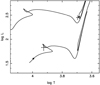 |
Fig. 12 Evolution tracks for 3.6 (above) and 2.4 M⊙ (below) in a theoretical HRD, with the positions of the γ Per components (see text for details). The age marks (black dots) refer to 257 Myr, the approximate age of the G giant in its central helium-burning phase. |
6 Discussion and conclusions
Summarizing the chromospheric line absorption modelling and analysis, we clearly detected a chromosphere in pure Ca II K line absorption in the eclipsing binary γ Per. It is slightly redshifted, as it originates in the rest frame of the G giant. We find a relatively small chromospheric density scale height of only 0.17 GM (see Table 3), the smallest of all ζ Aur systems with total eclipses, while the detectable extent of the chromosphere is about one A-star radius (3.9 R⊙). In that respect, γ Per confirms earlier findings from the chromospheric eclipses of similar ζ Aurigae-type binaries HR 2554 and HR 6902, which have a late G-type bright giant as well. In all these cases, the chromospheres are different from the much more extended chromospheres of the K supergiants of the classical ζ Aurigae systems (Wright 1970).
With an effective temperature around or just below 5000 K and a mass of about 3.6 M⊙, the late G-type giant of γ Per is most likely in its central Helium burning phase. Since the age of its companion is clearly larger and given the unusually large eccentricity as well as the large semi-major axis of the present orbit, the system could have formed by a capture event. Hence, we may speculate that the initial orbit might have been even more eccentric. In that case, an episode of angular momentum transfer around the time of a maximum RGB giant radius could have occurred, centred on periastron passages, where the giant’s rotation was slowed down. This might have helped to enlarge the periastron distance of the companion star and reduce the initially extreme eccentricity of its orbit to its present value.
This possibility added perhaps to a recent slow-down by magnetic braking of the giant rotation during its time spent in the central Helium burning phase, much as the two lesser active Hyades giants (see Schröder et al. 2020). Either one of these possibilities or a combination of both is consistent with the low activity found for the giant of γ Per, which compares to one of the inactive Hyades K giants ϵ Tau.
Hence, whatever leads to the present state, the γ Per late G-type giant is a perfect test case for the physics of inactive chromospheres and their properties, and what shapes them in the absence of an abundant magnetic field. In that sense, we are not surprised by how well the chromosphere of the γ Per giant and its extent match with the similar cases of HR 2552 and HR 6902, as discussed above, all in the transitional region of the HRD between coronal giants and those with cool winds.
The aforementioned “dividing lines” have been shown to not strictly divide the HRD into coronal and non-coronal cool wind giants because very active giants do show coronal plasma emission. It seems, however, that these lines’ orientation in the HRD reflects some fundamental physics of the inactive chromosphere. Extent and density scale heights appear to be related to the relative vertical distance from these lines, as was already pointed out by Schröder (1990). We suggest that therefore these lines reflect, where in the HRD the Athay point is not met any more by the cooler giant’s inactive chromospheres. This upper end of the chromosphere is where the neutral hydrogen reservoir and radiative cooling rates collapse and give way to the temperature jump into the corona, as known from the Sun (Athay 1981). In fact, for giants, we expect that to coincide in the HRD with the ‘Ca II dividing line’, because as shown above, late G giants still show evidence for some kind of weak corona, even without a high degree of activity.
In terms of chromospheric physics, comparing the extent and density scale heights of γ Per with the other giants and the Sun, we may see this G giant chromosphere as a low-gravity solar analogue, which still reaches its “Athay point”. This makes γ Per giant a particularly interesting, pivotal case. Compared to the Sun, it confirms the density scale-height Hd relation with gravity to be Hd ∝ ɡ−1.5, as derived from Ayres et al. (1975) for the lower chromosphere. This picture is consistent with finding much more extended chromospheres towards K-supergiants, as well as not resolving the chromosphere of the less luminous and slightly warmer G giant of τ Per, as well as earlier case studies of HR 6992 and HR 2554 (see Reimers et al. 1990; Schröder & Hünsch 1992).
The next eclipse of γ Per, from June 19 to 30 in 2034, will already be observable in the morning sky. Hopefully, space observations undertaken in June and July 2034 will answer that interesting question about extended transition region plasma as part of a low-energy corona suggested here by the reported XMM detection. It may be seen, as it was in HR 6902, in C IV and Si IV line absorption against the A star, which will then shine from behind again.
Acknowledgements
The authors are grateful for financial support from the bilateral project CONACyT-DFG No. 278156 and for the general support received by their home institutions. We also wish to thank Austrian AAVSO observer Wolfgang Vollmann for providing us directly with his photometric data, which contributed significantly to the precision of the height scale used for this eclipse of γ Per. We are also grateful to the XMM team to allow us a pointed observation as ToO to clarify the coronal nature of γ Per. Furthermore, we would like to thank the University of Guanajuato for the grant for project 003/2022 of the Convocatoria Institucional de Investigación Científica 2022. Finally, we thank the anonymous referee for raising some very helpful points to improve this paper.
References
- Ake, T. B. 2002, Atmospheric Eclipsing Binaries HR6902 and 22Vul, FUSE Proposal ID C138 [Google Scholar]
- Ake, T. B., & Griffin, E. 2015, Astrophys. Space Sci. Lib., 408 [Google Scholar]
- Athay, R. G. 1981, ApJ, 250, 709 [CrossRef] [Google Scholar]
- Ayres, T. R., Linsky, J. L., & Shine, R. A. 1975, ApJ, 195, L121 [NASA ADS] [CrossRef] [Google Scholar]
- Ayres, T. R., Brown, A., & Harper, G. M. 2003, ApJ, 598, 610 [NASA ADS] [CrossRef] [Google Scholar]
- Blanco-Cuaresma, S. 2019, MNRAS, 486, 2075 [Google Scholar]
- Budnik, F., Schröder, K. P., Wilhelm, K., & Glassmeier, K. H. 1998, A&A, 334, L77 [NASA ADS] [Google Scholar]
- Campbell, W. 1908, PASP, 20, 293 [NASA ADS] [CrossRef] [Google Scholar]
- Flower, P. J. 1996, ApJ, 469, 355 [NASA ADS] [CrossRef] [Google Scholar]
- Griffin, R. E. 2007, in Binary Stars as Critical Tools & Tests in Contemporary Astrophysics, 240, eds. W. I. Hartkopf, P. Harmanec, & E. F. Guinan, 645 [NASA ADS] [Google Scholar]
- Griffin, R., & Griffin, R. 1986, J. Astrophys. Astron., 7, 195 [NASA ADS] [CrossRef] [Google Scholar]
- Griffin, R. E. M., Griffin, R. F., & Schröder, K. P. 1990, ASP Conf. Ser., 9, 249 [NASA ADS] [Google Scholar]
- Griffin, R. E. M., Schröder, K. P., Misch, A., & Griffin, R. F. 1992, A&A, 254, 289 [NASA ADS] [Google Scholar]
- Griffin, R. F., Griffin, R. E. M., Snyder, L. F., et al. 1994, Int. Amateur Professional Photoelectr. Photom. Commun., 57, 31 [Google Scholar]
- Hauschildt, P. H., & Baron, E. 1999, J. Comput. Appl. Math., 109, 41 [NASA ADS] [CrossRef] [Google Scholar]
- Judge, P. G., & Carlsson, M. 2010, ApJ, 719, 469 [NASA ADS] [CrossRef] [Google Scholar]
- Kirsch, T., Baade, R., & Reimers, D. 2001, A&A, 379, 925 [NASA ADS] [CrossRef] [EDP Sciences] [Google Scholar]
- Linsky, J. L., & Haisch, B. M. 1979, ApJ, 229, L27 [Google Scholar]
- Maury, A. C., & Pickering, E. C. 1897, Ann. Harvard Coll. Observ., 28, 1 [NASA ADS] [Google Scholar]
- McLaughlin, D. B. 1948, AJ, 53, 200 [NASA ADS] [CrossRef] [Google Scholar]
- Mullan, D. J., & Stencel, R. E. 1982, in Advances in Ultraviolet Astronomy: Four Years of IUE Research, NASA CP-2238, eds. Y. Kondo, J. M. Mead, & R. D. Chapman, 235 [Google Scholar]
- Pols, O. R., Schröder, K.-P., Hurley, J. R., Tout, C. A., & Eggleton, P. P. 1998, MNRAS, 298, 525 [Google Scholar]
- Popper, D. M., & McAlister, H. A. 1987, AJ, 94, 700 [Google Scholar]
- Pourbaix, D. 1999, A&A, 348, 127 [NASA ADS] [Google Scholar]
- Reimers, D. 1982, A&A, 107, 292 [NASA ADS] [Google Scholar]
- Reimers, D., Baade, R., & Schröder, K. P. 1990, A&A, 227, 133 [NASA ADS] [Google Scholar]
- Rosas-Portilla, F., Schröder, K. P., & Jack, D. 2022, MNRAS, 513, 906 [NASA ADS] [CrossRef] [Google Scholar]
- Schmitt, J. H. M. M., Schröder, K. P., Rauw, G., et al. 2014, Astron. Nachr., 335, 787 [NASA ADS] [CrossRef] [Google Scholar]
- Schröder, K. P. 1990, A&A, 236, 165 [Google Scholar]
- Schröder, K. P., & Hünsch, M. 1992, A&A, 257, 219 [Google Scholar]
- Schröder, K. P., & Hünsch, M. 1994, A&A, 289, 893 [Google Scholar]
- Schröder, K. P., Griffin, R. E. M., & Hünsch, M. 1994, A&A, 288, 273 [Google Scholar]
- Schröder, K. P., Marshall, K. P., & Griffin, R. E. M. 1996, A&A, 311, 631 [Google Scholar]
- Schröder, K.-P., Pols, O. R., & Eggleton, P. P. 1997, MNRAS, 285, 696 [NASA ADS] [CrossRef] [Google Scholar]
- Schröder, K.-P., Schmitt, J. H. M. M., Mittag, M., Gómez Trejo, V., & Jack, D. 2018, MNRAS, 480, 2137 [CrossRef] [Google Scholar]
- Schröder, K. P., Mittag, M., Jack, D., Rodríguez Jiménez, A., & Schmitt, J. H. M. M. 2020, MNRAS, 492, 1110 [CrossRef] [Google Scholar]
- Vernazza, J. E., Avrett, E. H., & Loeser, R. 1973, ApJ, 184, 605 [NASA ADS] [CrossRef] [Google Scholar]
- Wilson, O. C., & Vainu Bappu, M. K. 1957, ApJ, 125, 661 [NASA ADS] [CrossRef] [Google Scholar]
- Wright, K. O. 1970, Vistas Astron., 12, 147 [CrossRef] [Google Scholar]
- Zahn, J. P. 1977, A&A, 57, 383 [Google Scholar]
- Zahn, J. P. 1989, A&A, 220, 112 [Google Scholar]
All Tables
Summary of the physical parameters of the γ Per components derived in this work, see text for more information.
Results from the line absorption modelling applied to the Ca II K line of the γ Per giant.
All Figures
|
Fig. 1 Merged eclipse light curve in the Johnson B filter of the 1990 (see + symbols of “GammaPerPhotomBecl1990plus2P” dataset) and 2019 photometry (see x symbols of “GammaPerPhotomBecl2019norm” dataset) on the 2019 JD scale (add 2458000 to x-axis values), by applying a best-fit period of 5329.08 days. TESS 2019 photometry is added, as well as spectrophotometry by TIGRE (“GammaPerPhotomTI-GREecl2019” data), and all 2019 data are scaled to the Johnson B eclipse depth of 1990. |
| In the text | |
|
Fig. 2 Flux-calibrated spectra of the composite spectrum from a phase outside eclipse (28 November 2019, black), G giant only in total eclipse (red) and subtraction to gain pure A star spectrum (blue), around the Ca II K line (3933 Å), which sees contributions from both stars. |
| In the text | |
|
Fig. 3 Subtracted spectra (A-star only) from outside eclipse (28 November 2019, black), chromospheric eclipse ingress (16. Nov. 2019, red), partial and chromospheric eclipse egress (25 November 2019, blue) and chromospheric egress (26 November 2019, purple), focussed on the Ca II K line. |
| In the text | |
|
Fig. 4 Ca II H&K and Hϵ region of the sole A star spectrum (blue) obtained from the subtraction of the out-of-eclipse spectrum of 28 November 2019 matched by a complete NLTE PHOENIX model spectrum for 8500 K (red), log ɡ = 3.5 and [Fe/H] = −0.2. |
| In the text | |
|
Fig. 5 Line absorption model (dashed line) applied to the giant’s chromospheric absorption (solid line) of the Ca II K line on the 16 November 2019 subtracted spectrum in ingress, normalized to the pure A star spectrum. |
| In the text | |
|
Fig. 6 Line absorption model (dashed line) applied to the giant’s chromospheric absorption (solid line) of the Ca II K line on the 25.11.2019 subtracted and normalized spectrum in egress, still in partial eclipse. |
| In the text | |
|
Fig. 7 Line absorption model (dashed line) applied to the giant’s chromospheric absorption (solid line) of the Ca II K line on the 26.11.2019 subtracted and normalized spectrum in egress. |
| In the text | |
|
Fig. 8 Column density vs. effective height from line absorption modelling with the estimated uncertainties of 0.5 dex in N and 0.1 Gm in height. See Table 3 for data. |
| In the text | |
|
Fig. 9 Comparison of the Ca II K line cores of the low activity Hyades early K-type giant ϵ Tau with the γ Per late G giant shows nearly perfect coincidence, demonstrating the low-activity nature of the latter despite its larger mass. While these spectra are virtually identical inside the Ca II K line, the gamma Per G giant’s spectrum contains the most noise. |
| In the text | |
|
Fig. 10 Soft X-ray photons detected by an 5 ksec XMM pointing in the OVΠ band (0.425–0.725 keV) at the position of γ Per (upper left circle) exceed the background count of 3 by statistically significant 7 extra photons. The lower right circle shows a separate, much harder source already detected by a 1990s pointing of ROSAT. The green striped triangle area is the source-free reference field which is used to determine the background. |
| In the text | |
|
Fig. 11 Positions of the giants in ζ Aurigae, 31 Cygni, 32 Cygni, 22 Vul, HR2554, HR6902 and τ Per, as well as of γ Per (red dot) in the observational HRD, in comparison with the ‘dividing lines’ between coronal (left) and cool wind (right) type stars, adopted from Schröder (1990) and Griffin et al. (1992). |
| In the text | |
|
Fig. 12 Evolution tracks for 3.6 (above) and 2.4 M⊙ (below) in a theoretical HRD, with the positions of the γ Per components (see text for details). The age marks (black dots) refer to 257 Myr, the approximate age of the G giant in its central helium-burning phase. |
| In the text | |
Current usage metrics show cumulative count of Article Views (full-text article views including HTML views, PDF and ePub downloads, according to the available data) and Abstracts Views on Vision4Press platform.
Data correspond to usage on the plateform after 2015. The current usage metrics is available 48-96 hours after online publication and is updated daily on week days.
Initial download of the metrics may take a while.