| Issue |
A&A
Volume 669, January 2023
|
|
|---|---|---|
| Article Number | A44 | |
| Number of page(s) | 13 | |
| Section | Planets and planetary systems | |
| DOI | https://doi.org/10.1051/0004-6361/202244460 | |
| Published online | 06 January 2023 | |
Mean motion resonance capture in the context of type I migration
1
Lund Observatory, Department of Astronomy and Theoretical Physics, Lund University,
Box 43,
22100
Lund, Sweden
e-mail: This email address is being protected from spambots. You need JavaScript enabled to view it.
2
Center for Star and Planet Formation, GLOBE Institute, University of Copenhagen,
ØsterVoldgade 5–7,
1350
Copenhagen, Denmark
Received:
9
July
2022
Accepted:
10
November
2022
Abstract
Capture into mean motion resonance (MMR) is an important dynamical mechanism because it shapes the final architecture of a planetary system. We simulate systems of two or three planets undergoing migration with varied initial parameters such as planetary mass and disk surface density and analyse the resulting resonant chains. In contrast to previous studies, our results show that the disk properties are the dominant impact on capture into MMR, while the total planetary mass barely affects the final system configuration as long as the planet does not open a gap in the disk. We confirm that adiabatic resonant capture is the correct framework for understanding the conditions leading to MMR formation because its predictions are qualitatively similar to the numerical results. However, we find that eccentricity damping can facilitate the capture in a given resonance. We find that under typical disk conditions, planets tend to be captured into 2:1 or 3:2 MMRs, which agrees well with the observed exoplanet MMRs. Our results predict two categories of systems: those that have uniform chains of wide resonances (2:1 or 3:2 MMRs), and those whose inner pair is more compact than the outer pair, such as 4:3:2 chains. Both categories of resonant chains are present in observed exoplanet systems. On the other hand, chains whose inner pair is wider than the outer pair are very rare and emerge from stochastic capture. Our work here can be used to link the current configuration of exoplanetary systems to the formation conditions within protoplanetary disks.
Key words: celestial mechanics / planets and satellites: dynamical evolution and stability / planets and satellites: formation / planet-disk interactions
© The Authors 2023
 Open Access article, published by EDP Sciences, under the terms of the Creative Commons Attribution License (https://creativecommons.org/licenses/by/4.0), which permits unrestricted use, distribution, and reproduction in any medium, provided the original work is properly cited.
This article is published in open access under the Subscribe-to-Open model. This email address is being protected from spambots. You need JavaScript enabled to view it. to support open access publication.
1 Introduction
Planets with a mass comprised between that of Earth and Neptune (called super-Earths) orbiting their star on orbits shorter than 100 days are the most common exoplanets discovered. It is estimated that close to 30% of Sun-like stars host a super-Earth (Fressin et al. 2013; Petigura et al. 2018). Many of these are in multiplanetary systems (see Zhu & Dong 2021 for a review). As planets grow in the protoplanetary disk, they raise spiral density wakes that exert a gravitational torque, leading to their migration (Lin & Papaloizou 1979; Goldreich & Tremaine 1980; Ward 1997; Armitage 2020). In this regime, known as type I migration, a super-Earth spirals in at a rate of about 1 m s−1 until it reaches the inner edge of the disk, where a positive torque stops the migration (Masset et al. 2006). Hydrodynamical 2d and 3D simulations of protoplanets embedded in a disk have constrained the migration rate as a function of the disk and planet properties (Tanaka et al. 2002; Tanaka & Ward 2004; Cresswell & Nelson 2006, 2008; Baruteau et al. 2014; McNally et al. 2020). The migration path depends on the properties of the disk and the planet. A steep temperature gradient can slow or even reverse migration (Paardekooper et al. 2010; Bitsch et al. 2015), or the accretion heat from the growing planet can modify the corotation torques (Benítez-Llambay et al. 2015). If the planet becomes more massive than a few tens of Earth masses, it will open a gap within the protoplanetary disk, slowing or even halting the migration (e.g. D’Angelo & Lubow 2010; Lega et al. 2021). This regime, called type II migration, has recently been interpreted as an extension of the type I migration by accounting for the reduced gas surface density within the gap (Kanagawa et al. 2018). In all cases, however, planet migration is a natural and unavoidable mechanism in the context of formation within the protoplanetary disk. Combined with planet growth through pebble accretion (Lambrechts & Johansen 2012; Johansen & Lambrechts 2017), planet migration is a dominant physical process that shapes the architecture of planetary systems (Johansen et al. 2019).
When multiple planets grow and migrate towards the inner edge of the disk, their gravitational interactions lead to capture into orbital resonances (Peale 1976; Goldreich & Tremaine 1980). Mean motion resonances (MMR) are configurations in which the planet period ratios are close to a ratio of integers. While the majority of close-in multiplanetary systems observed with the Kepler satellite are out of MMRs (Fabrycky et al. 2014), the existence of more than one hundred systems close to first-order MMRs (i.e. MMRs in which the period ratio is close to (k + 1)/k) is important evidence that migration occurs during the planet formation. Long MMR chains are a common feature in current planet formation simulations (Izidoro et al. 2017, 2021; Lambrechts et al. 2019), where many systems emerge from the disk phase in a configuration like this before they are broken soon after the disk dispersal. Izidoro et al. (2017) estimated that roughly 95% of the resonant chain should be broken to be consistent with the observations. Many mechanisms have been proposed to break resonant chains, such as intrinsic instability (Matsumoto et al. 2012; Pichierri & Morbidelli 2020), turbulence within the disk (Batygin & Adams 2017), a change in the planet or stellar mass (Matsumoto & Ogihara 2020), or tidal dissipation (Delisle & Laskar 2014), possibly enhanced by chaotic obliquities (Millholland & Laughlin 2019). Observed resonant chains provide a unique opportunity to probe the architecture of pristine configurations before orbital rearrangement. Studies of specific systems can offer a window on their formation conditions (Teyssandier & Libert 2020; Petit et al. 2020a; Hühn et al. 2021; Huang & Ormel 2022), or on the resonance dynamics and the capture mechanism (Pichierri et al. 2019; Charalambous et al. 2022).
Understanding the resonance capture has been the subject of numerous works over the past decades (see Batygin 2015 for a complete review). After the first studies (Goldreich & Sciama 1965; Goldreich & Soter 1966), a first analytical criterion was proposed in the context of the circular restricted three-body problem, developing the concept of probabilistic capture (Yoder 1979). The first general theory was developed using the formalism of adiabatic invariant by (Henrard 1982; see also Henrard & Lemaitre 1983; Lemaitre 1984). Batygin (2015) since simplified the framework and applied it directly to the context of capture of two massive planets undergoing migration. Capture is only possible for convergent migration, at a sufficiently slow pace. If the migration is slow enough to meet the adiabatic threshold (see Sect. 2.3), the capture is guaranteed for low eccentricities and has a finite probability for eccentric orbits. Mustill & Wyatt (2011) and Ogihara & Kobayashi (2013) numerically studied how the migration parameters affect the boundaries for capture and its probabilities. Other studies have focused on extending the capture theory to the non-adiabatic regime (Friedland 2001; Quillen 2006; Ketchum et al. 2011). After resonance capture, a system can nevertheless escape the resonance due to the over-stability of the fixed point (Papaloizou & Szuszkiewicz 2010; Deck & Batygin 2015; Xu et al. 2018) or be dynamically unstable (Pichierri et al. 2018). Moreover, systems in MMR can also be affected by general dynamical instabilities such as MMR overlap (Wisdom 1980; Deck et al. 2013; Petit et al. 2017, 2020b; Hadden & Lithwick 2018).
While many works have focused on understanding resonance capture, there is still a need for a general study of the capture in first-order MMR under a realistic setup. Most other numerical studies focus on the capture into a specific resonance and initialise the systems just outside of this resonance without studying the fate of a system if it were to cross the MMR. In addition, convergent type I migration for a pair of migrating planets is only possible when the outer planet is more massive or when the inner planet is halted by a planet trap. However, a configuration with a more massive outer planet often leads to an unstable resonance (Deck et al. 2013; Xu et al. 2018), and the case of a trapped inner planet has not been studied in detail, even though these configurations are supported by theoretical models (planet growth tracks; Johansen et al. 2019) and observations (uniform peas-in-a-pod systems; Weiss et al. 2018).
Our goal is to investigate the parameters governing migration and resonant capture to determine which MMRs are created as a function of the initial planetary and disk properties. While the typical conditions in the protoplanetary disk as well as the planetary masses can be roughly constrained, we explicitly probe how capture in resonance changes over a large set of parameters covering the regime in which planets experience type I migration, as well as the limits of this regime where planets start to open a gap. We analyse our results in the type I regime by considering the dynamically relevant variables (see Sect. 2.3), in order to compare our results to analytical criteria. Our study probes disk setups extending beyond the physically motivated conditions in order to contextualise the observational constraints. If the capture outcomes are widely different for unrealistic conditions in the protoplanetary disk and the planetary system (e.g. very high gas surface densities), we can use our results to consolidate our interpretation of the observed resonant chains. Thereby, our work can be viewed as a generalisation of the numerical works of Ogihara & Kobayashi (2013) and Xu et al. (2018), who studied the capture behaviour as a function of the migration prescriptions in a limited context.
In Sect. 2 we detail our model, the numerical setup, and the previously proposed analytical criteria for MMR capture. In Sect. 3 we present the results from our numerical experiments for two equal-mass planet systems for various masses, surface densities, and disk aspect ratios. We then generalise our results by considering three equal-mass planet systems in Sect. 4. We investigate in Sect. 5 the trends in capture condition between the different first-order MMRs by combining our previous results. Finally, in Sect. 6 we compare our findings to exoplanet resonant systems and discuss the theoretical implications of our study.
2 Numerical setup and theoretical motivation
2.1 Setup conditions
We used the N-body numerical integration library Rebound, with the integrator WHfast (Rein & Liu 2012; Rein & Tamayo 2015), to perform our simulations. We integrated coplanar systems with a 1 M⊙ star in a non-evolving protoplanetary disk of surface density ∑ and scale height h defined as
 (1)
(1)
 (2)
(2)
where s is the surface density profile index, β is the flaring index, ∑0 is the surface density at 1 AU, and h0 is the aspect ratio at 1 AU. Following Pichierri et al. (2018), we adopted the same values s = 1 and β = 0.25, which correspond to an optically thin disk (Hayashi 1981) assuming a constant accretion rate and constant α-viscosity parameter (Ida et al. 2016).
In the standard parametrised α viscous spreading prescription (Shakura & Sunyaev 1973), the gas accretion rate is connected to the surface density and aspect ratio through the relation
 (3)
(3)
where α is the viscous coefficient, and ΩK is the Keplerian velocity. In steady state, the accretion rate is constant in the disk, and we can evaluate Eq. (3) at r0 = 1 AU,
 (4)
(4)
where 𝒢 is the gravitational constant. The accretion rate is an observable that allows us to constrain the gas surface density, which is still poorly constrained in protoplanetary disks. Mass-accretion rate observations and inferred gas surface densities are consistent with α in the broad range 10−3–10−2 (Hartmann et al. 1998; Andrews et al. 2009). Within the disk lifetime, the accretion rate declines from 10−7 M⊙ yr−1 to 10−9 M⊙ yr−1 (Manara et al. 2016, 2022; Tazzari et al. 2017). Importantly, the accretion rate can be loosely connected to the system age during the formation phase. We emphasise, however, that we only infer a disk accretion rate to connect our results to observable quantities. In particular, the assumed value for a does not affect the results of our simulations because the disk is parametrised through its surface density and aspect ratio.
We considered a case where the inner planet is fixed at 0.1AU at the inner disk edge, while the outer planet migrates inward via type I migration from a position outside the 2:1 MMR with the inner planet. The initial positions of the planets were 0.1 and 0.2 AU unless specified otherwise. Fixing the inner planet at the inner disk edge provides a controlled setting in which the planets are captured into MMR at the same position and orbital period. Based on planet formation models, we can consider the migration to be sequential, meaning that planets grow and then migrate until they reach the inner disk edge one after the other (Izidoro et al. 2017), possibly entering and maintaining a MMR configuration.
Every integration lasted for one migration timescale of the outer planet. This is more than enough time for the outer planet to be captured in an MMR configuration as the planet would reach the inner disk edge if it were isolated. We did not integrate for longer because we do not focus on the long-term stability of the MMR. We chose a timestep of P(0.1 AU)/20 = 1.6 × 10⁻³ yr, which is sufficient for this type of setup. Moreover, we stopped the integration when the separation between the planets was smaller than one Hill radius. Smaller separations result in encounters or collisions and will not lead to a stable MMR configuration. Initial eccentricity and mutual inclinations were kept unchanged at zero as they are rapidly damped by the disk and do not affect MMR capture (Mustill & Wyatt 2011; Ogihara & Kobayashi 2013).
2.2 Planet migration
Within the protoplanetary disk, a protoplanet exchanges angular momentum with the gas and migrates (e.g. Armitage 2020). If the perturbation to the gas density remains weak and the planet does not open a gap, the mechanism is called type I migration (Tanaka et al. 2002; Cresswell & Nelson 2006; Baruteau et al. 2014). The disk-planet interaction is composed of two separate contributions: damping the orbit eccentricity, and the migration affecting the semi-major axis. More precisely, the eccentricity is dampened as
 (5)
(5)
and the contribution of the disk interaction to the semi-major axis dynamics is
 (6)
(6)
where p = 1 for low values of e (Pichierri et al. 2018). The timescales τa and τe are then defined as
 (7)
(7)
 (8)
(8)
where τwave is the typical timescale of type I migration (Tanaka & Ward 2004),
 (9)
(9)
fei,a and fei,e are functions describing the influence of the inclination and eccentricity terms, and n is the planetary mean motion. We used the expressions in Eqs. (11)–(13) of Cresswell & Nelson (2008). While more realistic torque expressions have been developed since (Paardekooper et al. 2010, 2011), they change the prefactor of the migration timescale τa by a factor of the order of unity, which varies slowly with the planet mass. This change would slightly affect the migration timescales for a given surface density, but not the relative migration speed between the planets. As we considered a wide range of masses and surface densities, changing the torque prescription would only affect the quantitative results moderately.
In the numerical simulations, the effects of damping e and a were applied to the planet acceleration as
 (10)
(10)
where r and v are the planet position and velocity, respectively.
The inner edge of the disk acts as a planet trap (Masset et al. 2006) through the sharp change in surface density. We modelled a planet trap based on Pichierri et al. (2018) by dividing τa with a factor
 (11)
(11)
which was activated only within a narrow distance from the exact position of the inner disk edge, rie, measured as the scale height hide at ride. The inner disk edge was set at ride = 0.1 AU as suggested by Izidoro et al. (2017) and Brasser et al. (2018) to be common for solar-type stars. Both these effects were implemented via Reboundx, a complementary software that enables implementation of non-gravitational effects as forces in Rebound simulations (Tamayo etal. 2020). The implementations used in this work were made available as part of the Reboundx library1.
Beyond a certain mass, a planet opens a partial gap in the disk, which changes the nature of the migration (Lin & Papaloizou 1993; Ward 1997; Crida & Morbidelli 2007; Baruteau & Papaloizou 2013; Kanagawa et al. 2015, 2018). This regime is called type II migration, and the migration rate is no longer determined by Eq. (7). Instead, the resulting torque onto the planet depends on the gap depth and the disk properties, in particular the turbulent viscosity parametrised by α. Kanagawa et al. (2018) proposed a framework for gap-opening planet migration where the migration rate from type I can be amended to account for the gap by replacing the unperturbed gas surface density in Eq. (7) by the surface density at the bottom of the gap. The surface density inside the gap ∑gap is related to the unperturbed gas surface density ∑uπp as
 (12)
(12)
where K is given as
 (13)
(13)
h is the gas scale height (Eq. (2)), and α is the Shakura-Sunyaev turbulent viscosity parameter.
For values of K higher than 20 (Kanagawa et al. 2018), the surface density is significantly affected and the migration is slowed by the gap. From Eq. (13), the transition mass beyond which type I migration is unrealistic is
 (14)
(14)
To account for the transition to type II migration, we replaced the surface density in the expression of τwave by ∑gap given in Eq. (12), which modifies both τe and τa as was done by Kanagawa & Szuszkiewicz (2020). The ratio τe/τa remains unaffected by this modification. While no semi-analytical expression exists for the eccentricity damping during type II migration, this approach is supported by hydrodynamical simulations, which show a rapid damping of the eccentricity provided it remains lower than the disk aspect ratio (Bitsch & Kley 2010; Duffell & Chiang 2015).
2.3 Condition for resonant capture
For each set of simulations we ran, we analysed whether the systems reached a first-order MMR and if they did, which MMR they reached. At the end of the integration, all systems were either trapped in an MMR or became unstable. We removed unstable systems by discarding systems where the final configuration is Hill unstable (Marchal & Bozis 1982; Petit et al. 2018). Using the circular approximation (Gladman 1993), Hill-unstable systems verify
 (15)
(15)
where
 (16)
(16)
is the planet-to-star mass ratio. The circular approximation is sufficient because systems out of MMRs circularise rapidly with respect to the migration timescale.
For a pair of planets exactly at the resonance k + 1:k, we have
 (17)
(17)
By solving this equation for k, we determined the closest MMR by computing a continuous resonant index
 (18)
(18)
Denoting by [κ] the closest integer to k, we measured the distance to the resonance by computing (e.g. Pichierri et al. 2019)
![Mathematical equation: ${\rm{\Delta = }}{{\left[ \kappa \right]} \over {\left[ \kappa \right] + 1}}{{{P_2}} \over {{P_1}}} - 1.$](/articles/aa/full_html/2023/01/aa44460-22/aa44460-22-eq19.png) (19)
(19)
Here, Δ is positive for pairs of planets that are wide of the MMR. We considered that a planet is trapped in an MMR if 0 < Δ < 0.03. While this criterion is not sufficient in general, we find that it gives a correct representation of the dynamical state while planets migrate through the disk. We integrated the system for a timescale at least three times longer than the time it takes to be trapped in an MMR. If the planets were not trapped in MMR, the outer planet would cross the resonances, leading to scattering events or to collision with the inner planet. Furthermore, analysis of selected systems from our simulations showed that the resonant angle librates for systems verifying the Δ criterion.
The theory of adiabatic invariants (Henrard 1982, 1993) has shown that capture into resonance is a probabilistic event in general (see Batygin 2015, and references therein for a current review). The particular structure of first-order MMR (Henrard & Lemaitre 1983; Sessin & Ferraz-Mello 1984) ensures, however, that capture is guaranteed for convergent planets on close to circular orbits. At low eccentricity, it is possible to enter the resonance without crossing the separatrix. The dynamics are considered adiabatic if a (quasi)-constant of motion of the non-dissipative problem (i.e. a parameter) evolves slowly with respect to the dynamical timescales of the rest of the system. This is the case for the dynamics of two planets near a first-order MMR undergoing semi-major axis damping (Henrard & Lemaitre 1983). However, eccentricity damping does not conserve the resonant variables, which breaks the adiabatic assumption (Goldreich & Schlichting 2014).
In the context of resonant motion, Batygin (2015) proposed that adiabatic capture can take place if the resonance libration period is shorter than the migration time across the resonance,
 (20)
(20)
where  is the relative migration rate, and
  is a function depending on the Laplace coefficients (Laskar & Robutel 1995; Murray & Dermott 1999) that can be approximated at the resonance loci as
  k (Deck et al. 2013). While type I migration is not an adiabatic process due to the eccentricity damping, criterion Eq. (20) provides a good analysis framework for understanding the mechanism at play during resonance capture. In this framework, the critical τa,crit for which capture is possible scales as
  . Ogihara & Kobayashi (2013) proposed the same scaling based on numerical simulations.
In the context of type I migration, the disk surface density acts as a proxy for the migration timescale. As Batygin (2015), using Eq. (20) and assuming that the inner planet is trapped at the inner edge, we determined a critical surface density depending mainly on k, εp and h0, below which capture into the k+1: k MMR is possible,
 (21)
(21)
where r0 = 1 AU, ζ = m1/m2. Analytical theory predicts  , which should lead to a significant variation in the capture condition for a given surface density if the planet mass is varied over several orders of magnitude.
When accounting for type II migration, the simple functional form of Eq. (21) can be preserved by replacing ∑0 with
 (22)
(22)
In the chosen disk model, K still depends weakly on the orbital radius because the disk is flared. Neglecting this variation, we can treat the capture in MMR of gap-opening planets in the framework of type I migration as if the planet were embedded in a reduced-mass disk with a surface density given by ∑0,gap.
3 Resonance capture for two-planet systems
3.1 Role of the surface density ∑0 and the planet mass mp
Based on the theoretical criterion Eq. (21), we first focused on the impact on the capture in MMR from the surface density ∑0 and the planet mass by varying the two over a wide range of values, even beyond the regime in which type I migration is valid. We varied the planet mass mp = m1 = m2 over two orders of magnitude from 10−6 M⊙ to 10−4 M⊙. For α = 10−2 and h0 = 0.033, Eq. (14) predicts that planets migrate in the type I regime for masses lower than 3.3 10−5 M⊙. The chosen value of α is consistent with our setting because the planets lie close to the inner edge of the disk where the magnetorotational instability is active and maintains the turbulence (e.g. Johansen et al. 2006; Bai & Stone 2011). We varied the surface density at 1 AU, ∑0, from 4 × 10² g cm−2 to 5 × 10⁴ g cm−2. This range covers the typical surface densities of forming disks inferred from accretion rates (Hartmann et al. 1998), but is extended to higher values to probe the rapid migration regime where more compact resonances can be formed. The differences in trends are more robust over a wider range, and the whole picture becomes clearer. In particular, high ∑0 values show the relation between different resonances, and probing high masses is necessary because the exponent of the analytical criterion is weak (one-third). Exploring the capture outcome beyond the regime compatible with observational constraints gives a consistency check in the comparison with the observations. If the expected conditions during planet formation are compatible with the observations but unphysical initial conditions lead to the formation of resonances that are not observed in exoplanet systems, we can conclude that the observed MMRs reinforce our constraints on the protoplanetary disk. Moreover, we benefit from the extended explored parameter space in our comparison between the analytical trends and the numerical simulations. We ran 170 000 simulations exploring this 2D (mp, ∑0) parameter space. As explained in Sect. 2.1, the planet masses were equal, and the inner planet was fixed at the inner disk edge. In all the simulations, the aspect ratio at 1 AU was ho = 0.033, and we computed K (Eq. (13)) at the initial position of the outer planet.
Figure 1 shows the final value of κ (Eq. (18)) for the 170 000 individual integrations as a function of the surface density ∑0 and the planet mass mp. We connected the surface density to the accretion rate of a viscous disk with Eq. (4), assuming α = 10−2 (Hartmann et al. 1998; Hasegawa et al. 2017). Initial conditions in which the outer planet encountered the Hill stability limit due to fast migration, leading to unstable systems, were removed from the figure and are plotted in white. Red points correspond to systems out of resonance for criterion Eq. (19). For κ < 10, the transitions between the resonances are very clear, and the resonant index increases with ∑0. A higher surface density leads to a faster migration, bringing the planets to a smaller orbital separation (and thus higher resonant index) before capture becomes possible. For high resonant indexes (κ ≳ 10), the transitions are not as sharp because of resonance overlap. These configurations only appear possible for unrealistic surface densities (∑0 ≳ 104 g/cm2), and we therefore did not analyse the results in this region further.
We note the transition mass mtransition = 3.3 × 10⁻⁵M⊙ to the type II regime (Eq. (14)) with a vertical dashed line. For a given surface density, planets with mp ≳ mtransition tend to be trapped in lower-index resonances with respect to planets in a purely type I migration regime due to the reduced migration rate. For higher masses, we expect all planet pairs to be trapped in a 2:1 resonance.
A better insight into the dynamics and MMR capture can be obtained by plotting the resonant index as a function of the rescaled surface density to account for the gap opening Σ0,gap. The migration rate is linear in Σ0,gap, and the planet mass mp and this rescaling allow us to treat any system within the simpler type I migration framework. We plot in Fig. 2 the same simulations as in Fig. 1, but as a function of Σ0,gap.
Inspired by criterion Eq. (21), we note  , the surface density below which a system is captured into the k+1:k resonance. Following the method from Ogihara & Kobayashi (2013), the transition surface densities
  were obtained by fitting for each mp the condition κ(∑0) < k + 1/2 as a probability function,
 (23)
(23)
As the transitions are sharp for low resonant indexes, the value of γk is high, and we do not report these transitions.
Figure 2 shows two different trends for the transitions between the different resonances. In most of the investigated parameter range (mp ≳ 3 × 10⁻⁶ M⊙), for all κ ≤ 10, the values of  show no dependence on mp and the planet-to-star mass ratio εp, and they occur at fixed surface density values for all κ. The transition surface density is constant across two orders of magnitude in mp. According to the capture criterion Eq. (20), we should have
  and thus observe a significant change in transition surface density with the planet mass. For planets in the regime of masses that is relevant for type I migration, our simulations show the limits of the adiabatic framework.
For mp ≲ 3 × 10⁻⁶ M⊙, the transitions show a weak mp dependence. Fitting  as a power law of mp for values lower than 3 × 10⁻⁶ M⊙ and 2 ≤ κ ≤ 10, we obtain
  , which is still lower than the one-third value found analytically by Batygin (2015). It remains possible that at lower masses, the transition power exponent could match the analytical criterion. This regime is not relevant for planet formation, however, because planets grow to higher masses before they migrate significantly (Johansen et al. 2019).
For low-mass planets (mp ≲ 3 × 10⁻⁶ M⊙), the transition between the 2:1 and the 3:2 MMR follows a different pattern than higher-index transitions as there are no systems in the 2:1 MMR for these masses. We interpret this feature as a sign of the over-stability of the 2:1 resonant centre in this regime. The linear stability analysis of the resonance fixed point (Deck & Batygin 2015) has shown that the resonant variable can spiral out and eventually escape the resonance. The stability of the fixed point is mainly governed by the mass ratio of the planets (a smaller inner planet can lead to overstability, while a more massive inner planet usually stabilises the resonance), the specific resonance (the 2:1 MMR is more sensitive than higher indexes), and the ratio of eccentricity dissipation between the two planets (which in the case of type I migration is roughly proportional to the planet mass ratio). Xu et al. (2018) have shown that the more realistic migration and eccentricity-damping rates from Cresswell & Nelson (2008) can allow overstable configurations to remain trapped in the MMR, but with a finite libration amplitude. We note that the shape of the transition we observe in Fig. 2 is similar to the shape of the overstable region in Fig. 3 of Xu et al. (2018). In the case of resonance escape, the planets resume migration towards inner MMRs until a stable MMR is encountered (Deck & Batygin 2015). In this case, the planets escape 2:1 and stabilise in 3:2. In Appendix A, we analyse the role of the overstability of the resonance further by considering the case of two planets with unequal mass, as well as the case of two migrating planets. As predicted by Deck & Batygin (2015), our simulations show that the overstability occurs for all resonances when the outer planet is more massive than the inner planet, provided that the planet-to-star mass ratio is lower than a critical value.
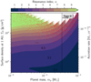 |
Fig. 1 Final continuous resonance index k (Eq. (18)) of two equal-mass planets as a function of the surface density Σ0 at 1 AU and the planet mass mp. The inner planet is fixed at the inner disk edge (0.1 AU), while the outer planet migrates from 0.2 AU. Systems that do not satisfy 0 < Δ < 0.03 are considered not in resonance and are plotted in red. Hill-unstable systems are removed and are plotted in white. The dashed line indicates the transition mass (Eq. (14)) to the regime of type II migration. The accretion rate displayed on the right axis is computed from Eq. (4) assuming a viscous parameter α = 10−2. |
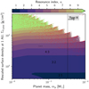 |
Fig. 2 Final continuous resonance index κ (Eq. (18)) of two equal-mass planets as a function of the rescaled surface density Σ0,gap (Eq. (22)) and the planet mass mp. Using the rescaled surface density allows highlighting the dynamically relevant quantity for the resonant capture. |
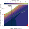 |
Fig. 3 Continuous resonance index κ for a pair of 10−5 M⊙ equal-mass planets as a function of the rescaled surface density Σ0,gap (Eq. (22)) and the disk aspect ratio h0. The green line verifies Σ0 ∝ h2, corresponding to a constant migration timescale. The yellow line is an example of the fitted |

3.2 Influence of the disk aspect ratio h0
For a planet undergoing type I migration, we showed that the planetary mass has a weak impact on MMR capture. We now kept the planetary mass constant at mp = m1 = m2 = 10−5 M⊙ (below the type II transition mass for h0 = 0.033) and instead investigate the role of the disk aspect ratio, h0, in the final resonant configuration. From Eq. (7), we have that  , so that systems with equal migration timescales lie on curves verifying
  . According to criterion Eq. (20), we expect the resonance transitions to have a similar dependence. When we vary h0, we also change the relation between τe and τa since
  . As a result, we can test whether τe impacts the MMR capture. The disk aspect ratio is much more constrained than the other considered parameters. Understanding its influence on the MMR capture is thus more relevant from a theoretical perspective. Our previous setup showed that the transition to the type II regime tends to hide dynamical features such as the power-law trend in the transition surface densities. We thus decided to present the results of this section only as a function of the rescaled surface density ∑0,gap. The transition to the type II regime can also be expressed as a critical aspect ratio. For a planet of mass mp = 10−5 M⊙ at 0.2 AU, the planet opens a gap if the aspect ratio h0 < h0,transition = 0.02.
We varied the rescaled surface density ∑0,gap from 10 g cm−2 to 5 × 10⁴ g cm−2 and h0 from 0.01 to 0.1, simply spanning an order of magnitude around the typical value taken as realistic in the literature. We integrated 80, 000 equal-mass two-planet systems and present the results in a 2D grid, where each pair corresponds to a combination of h0 and ∑0,gap. Again, the inner planet was initialised at the inner disk edge, and the planets had the same mass.
Figure 3 shows the final value of κ as a function of ∑0,gap and h0. Similarly, the white points correspond to unstable systems, and the red dots are systems considered out of resonance. The green line verifies  to help visualise configurations with an equal migration rate. We see similarities with Fig. 2 in the behaviour of ∑0,gap and in the sharpness of the transitions between the resonances. A higher surface density ∑0,gap or a thinner disk (smaller h0) lead to faster migration and so to capture into higher k MMRs. The transitions are sharp for indexes κ ≲ 10. For the thicker disks (h0 > 0.033), we observe a break in the power-law trend as no systems end up in the 2:1 MMR due to the overstability of the fixed point.
We fitted the transition between the resonances and obtained that  , instead of the scaling
  expected from the analytical modelling. The exponent 3.02 ± 0.01 suggests that the eccentricity damping also plays a role in the capture in MMR. This result is surprising because Ogihara & Kobayashi (2013) found no significant trend when they studied the impact of τe on the transition between capture in different MMRs. A possible explanation may be that Ogihara & Kobayashi (2013) did not consider the case in which the eccentricity damping of both planets varies at the same time.
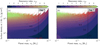 |
Fig. 4 Continuous resonant indexes κ12 (a) and κ23 (b) of the inner and outer pair of planets as a function of mp and Σ0 for three equal-mass planet systems. The innermost planet is initialised at the inner disk edge, while the other two planets migrate from 0.2 and 0.3 AU, respectively. The initial conditions are otherwise identical to the first run presented in Fig. 2. The dashed black line indicates the gap-opening threshold at 3.3 × 10⁻⁵ M⊙. |
4 Three-planet resonant chains
Resonant chains often contain more than two planets. It is thus natural to test whether the results found in previous subsections hold for more complex systems. We used a three-planet coplanar system with the same conditions as in the run presented in Sect. 3.1 to determine whether the qualitative behaviour and relation between Σ0 and mp change. In this run, the innermost planet was fixed at the inner disk edge at 0.1 AU, the middle planet migrated inward from 0.2 AU, and the outermost planet migrated from 0.3 AU. The capture is thus sequential: The first pair of planets is captured before the outer planet joins the chain, which might affect the inner pair. The initial parameters Σ0 and mp span the same 2D grid.
We plot in Fig. 4 the resonant indexes κ12 and κ23 for the respective planet pair. The overall qualitative behaviour is preserved as we do not observe a dependence on mp for  before the transition to the type II regime. However, the transitions between the resonances are noisier, particularly for the outer pair. Because the outer planet is captured while the inner pair of planets is already in resonance, the middle planet is no longer on a circular orbit, which makes the capture of the outer planet no longer deterministic (Henrard 1982; Batygin 2015). We can note that the resonant index is more stochastic for lower planetary masses, probably because the resonance islands are smaller.
The inner pair can also be disrupted by the subsequent capture of the outer pair. We note that the surface density transitions  for the inner pair are 22% lower on average than the same transition in the two-planet case (see the next Sect. 5, and Appendix B). The difference between the resonant indexes of the inner pair and the two-planet result from Sect. 3.1 is displayed in Fig. B.1. Within the considered parameter space, 36% of the inner pairs are trapped in the next index resonance compared to the two-planet case. By studying the inner-pair resonant indexes before the capture of the outer planet, we note that the inner pair behaves similarly to the two-planet case. However, the originally formed resonance can be disrupted by the arrival of the outer planet for systems close to the surface density transition. In this case, the migration resumes until the inner pair is captured into the next resonance. The picture is slightly different for the outer pairs. We plot in Fig. B.2 the difference between the outer-pair resonant indexes and the two-planet system resonant indexes. We find that the transitions occur almost at the same surface densities as in the two-planet case, but with a significant scattering around the transition; 2% of the pairs are trapped in a tighter resonance and 26% in a wider resonance with respect to the two-planet case.
We also quantified the intra-system uniformity. We plot in Fig. 5 the difference of resonant index κ12 − κ23 between the inner and the outer pair of each system. For the considered parameter space and among all systems in which both pairs of planets are in resonance, we find that only 39% form a uniform chain with κ12 = κ23. For non-uniform chains, we find that κ12 = κ23 + 1 in 57% of the cases and κ12 = κ23 + 2 in 3.3% of the cases. Systems in which the inner pair is wider than the outer pair account for less than 1% of the chains. However, this general picture is slightly misleading when the focus is on the low-index resonances. We find that whenever the inner pair is in a 2:1 resonance, all the systems form a Laplace 4:2:1 chain. Similarly, 98% of the systems in which the inner pair is in a 3:2 resonance are 9:6:4 resonant chains. On the other hand, only 16% of the chains in which the inner pair is trapped into a higher-index (κ12 ≥ 3) resonance are uniform chains.
Our findings show that the two-planet results from the previous subsections can be generalised to more complex systems. In particular, we interpret uniform chains as a consequence of the disk properties being the dominant parameters leading to the capture into a specific resonance. We expect that systems with four or more planets would also show the same qualitative behaviour. However, resonant systems with many planets can become unstable due to excitation from secondary resonances, which complicates the picture. The mass threshold for this type of instability decreases with increasing k and with increasing number of planets (Pichierri & Morbidelli 2020).
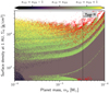 |
Fig. 5 Difference κ12 − κ23 of the inner and outer pair continuous resonant indexes as a function of the planet mass mp and the surface density Σ0. As in previous figures, the red dots correspond to systems far from resonance, and the dashed black line corresponds to the gap-opening threshold (3.3 × 10⁻⁵M⊙). |
5 Transition surface density ∑tr as a function of the resonance index k
We combined the results from our different setups to study the trend in the resonant index for the transition surface densities. Equation (21) predicts that  scales asymptotically as k1.55. However, for 2 ≤ k ≤ 10, a power-law fit of Eq. (21) leads to a slope of 1.34. We excluded the 2:1 resonance from the trend analysis due to its unique dynamics (Beauge 1994). We fitted
  as described in Sect. 3.1 for the results presented above. From the setup displayed in Fig. 2 and the three-planet systems, we used the constant transition regime for mp ≳ 10−5 M⊙. As seen in Sect. 3.2, the transition surface density is not constant with h0, but we have
  . We therefore modelled the aspect ratio dependence from the Sect. 3.2 results by taking the average value of
  such that the reported value was comparable to the other setups. The chosen planet mass and disk aspect ratio place us in the type I regime, where we can neglect the effect of the gap opening.
We plot in Fig. 6 the transition surface densities as a function of k from our simulations as well as the analytical prediction Eq. (21) for εp = 2 × 10⁻⁵ and h0 = 0.033. The analytical prediction is smaller by a factor 2 to 3 than the numerical fits, but the actual factor is mostly determined by the choice of aspect ratio and mp because the scaling found numerically differs from the analytical scaling. We observe that all results follow a similar power-law trend for k ≥ 2 with a slope of 1.42 ± 0.04, which is consistent with the analytical prediction. This agreement shows that the dynamics of the resonant motion are likely well approximated by the first-order model used in (Batygin 2015). On the other hand, the discrepancy in the mass and aspect ratio trends suggests that the migration timescale is not the only parameter governing the resonance capture, but that the eccentricity damping should play a significant role. Similarly, the analytical surface transition being smaller than the numerical fit can be interpreted by noting that the actual capture mechanism is more robust than the adiabatic condition predicts.
Moreover, Fig. 6 shows that the transition surface density ∑tr,12 for the inner pair of planets in the three-planet case is lower than in the two-planet case. As explained in Sect. 4, the outer planet compacts the inner pair when it enters in resonance with the middle planet.
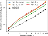 |
Fig. 6 Transition surface densities |


6 Comparison to observed chains
Our results show that for planets below the type II mass transition, capture in resonance at the inner edge of a disk is mainly ruled by the disk parameters rather than the planet properties (although in the case of an inner less massive planet, fix-point overstability can play a role, as seen in Appendix A). Figure 2 shows that for type I migrating equal-mass planets, there is almost no dependence on the planet mass. In the adiabatic framework, the MMR capture is possible if the migration time across the resonance is longer than the resonance libration period (Batygin 2015). We showed that this model provides a qualitative explanation for the transition between successive resonances. However, we see that the eccentricity damping likely plays a significant role as capture is also possible for systems in which the libration timescale is longer than the resonance crossing time. Beyond two-planet systems, the capture properties are not strongly affected in longer chains. For an inner pair of planets with a low-resonance index (2:1 or 3:2 MMR), the chain is most likely uniform, that is, with the outer planet pair having a similar index. For a higher index, the inner pair is usually tighter than the outer pair. We can use these results to link the observed exoplanets to the formation conditions of resonant chains.
While our simulations were performed with a planet trapped at the inner disk edge at 0.1 AU around a solar-mass star, it is quite straightforward to rescale the problem to generalise our results. Changing the stellar mass amounts to changing the mass units of our simulations, and the surface density and planet masses should be rescaled accordingly. Changing the mass units while keeping the same gravitational constant and time units requires the modification of the length unit. Capture beyond the inner disk edge at an arbitrary distance can also be predicted from our simulations by using the surface density at the capture location instead of its value at 0.1 AU.
Planet migration is a well-understood process that must take place in the protoplanetary disk from its formation to its photoevaporation. During the early growth phases, however, planets mostly grow, but they barely move because the growth timescale is shorter than the migration one (Johansen et al. 2019). The growth from lunar-mass embryos to super-Earths is governed by the pebble-mass flux in the inner region of the disk. Low flux means slow growth, thus little migration during the disk lifetime. In particular, Lambrechts et al. (2019) showed that super-Earth embryos start to migrate only after half a million years. The typical surface densities at 1 AU during the disk lifetime can be derived from the disk accretion rate. If we assume a viscous spreading parameter α = 10−2, a typical class II disk surface density at 1 AU ranges from ≃2000 g cm−2 to ≃ 10 g cm−2, when the accretion rate drops from a few 10−7 M⊙ yr−1 to 10−9 M⊙ yr−1 over the lifetime of the protoplanetary disk. Figure 1 shows type I migration in this range of surface densities leads to a trapping into 3:2 or 2:1 MMRs for most systems. In particular, 3:2 MMR are formed for  between 3 × 10⁻⁸ M⊙ yr−1 to 2 × 10⁻⁷ M⊙ yr−1, which roughly corresponds to the first one million years of the disk lifetime (Testi et al. 2022). Within the inner parts of the disk that we consider here, there is more than enough time to grow protoplanets until they start migrating within that timeframe. Our simulations provide loose evidence that super-Earth formation likely occurs early in the evolution of the protoplanetary disk. The surface density of protoplanetary disks is not very well constrained because the constraints on the viscous parameter a or the role of magnetic winds (Tabone et al. 2022) that can affect the profile of the disk are poorly constrained. In particular, slightly higher surface densities are not ruled out, which could also explain the observed higher-index resonances as a result of planet formation at later evolutionary stages.
Next, we compared our results to the observed multiple exoplanet resonant chains using the NASA exoplanet archive2. Following the same approach as Pichierri et al. (2019), we selected all systems that contained a pair of planets with 0 < ∆ < 0.03. The selection condition only enforces that the planet pairs are slightly wide of commensurability and not that they are actually in resonance. However, detailed dynamical analyses of some of these systems, in particular the longer chains, have shown that they are still in resonance (e.g. Trappist-1, Agol et al. 2021, or TOI-178, Leleu et al. 2021). Moreover, tidal effects during the system lifetime can cause resonant systems to settle slightly wide of the resonance configuration in which they were originally captured (Delisle & Laskar 2014; Millholland & Laughlin 2019). Given the fragility of resonant chains (Izidoro et al. 2021; Raymond et al. 2021), we can expect these chains to be close to their original state. We find 158 pairs close to a first-order MMR within 127 systems.
The majority of the observed exoplanet pairs close to MMR are isolated (i.e. not part of a longer chain). Among them, we find 52 pairs close to the 2:1 MMR, 67 pairs close to the 3:2 MMR, and 39 close to a higher-index resonance. This distribution of MMRs is consistent with the capture of planets undergoing migration in a typical protoplanetary disk because the surface density needed for the capture in a k ≤ 2 MMR is comparable to the typical surface density in a protoplanetary disk. However, it is harder to connect a specific pair to the disk properties at the time of the formation. Instead of considering individual resonant pairs, we now focus on three and more planet chains, as we can study how the trends in an individual system compare to the results from Sect. 4. As a result, we only kept the systems containing two consecutive resonant pairs.
The 15 selected systems are plotted in Fig. 7 as a function of their orbital period. The size of the planets corresponds to their radius when available, or we defined the planet radius as Rp = R⊕(Mp/M⊕)1/3 for illustrative purposes. When a pair of planets is resonant, we link the two planets with a line segment of colour according to the resonance index. The planet is plotted in grey when it is out of resonance.
We can divide the selected systems into three broad categories. One system subset is composed of low-index (3:2 and 2:1) uniform resonant chains (HD 158259, Kepler-24, K2-138, Kepler-31, and GJ 876). The 4:2:1 chains are composed of massive planets. Kepler-31 b, c, and d have a radius of 5.5 R⊕, 5.3 R⊕, and 3.9 R⊕, respectively (Fabrycky et al. 2012). GJ 876 c, d, and e have reported minimum masses of 227 M⊕, 723 M⊕, and 14 M⊕, respectively (Rivera et al. 2010). In both cases, the masses or radii of the two innermost planets of the chains are comparable to those of Saturn or Jupiter. These planets likely opened a gap in their protoplanetary disk, which slows their migration and allows the capture into the 2:1 resonance (Kanagawa & Szuszkiewicz 2020), as shown in Fig. 1.
Moreover, there are three-planet chains with a higher-index inner pair, that is, chains of the form k+2:k+1:k (Kepler-226, Kepler-60, Kepler-431, Kepler-305, and K2-268). In these systems, the inner pair can initially be in the same resonance as the outer pair before it is pushed into the higher-index MMR during the capture of the outer planet. These two categories are consistent with the simulations presented in Sect. 4. Uniform chains tend to have low resonant indexes, whereas higher-index resonances belong to k+2:k+1:k chains.
Finally, the last category is composed of systems out of the previous two patterns (Kepler-444, Kepler-80, Trappist-1, Kepler-223, and TOI 178). These systems have a more complex architecture with longer chains. As resonant planets have a non-zero eccentricity, the capture of a new planet in an already existing chain can become probabilistic (Batygin 2015) and create non-uniform chains. The existence of these systems is not incompatible with our results, howver. In most of these systems, we only observe a single pair that differs from the other resonances. Moreover, detailed studies of these particular systems have shown that they are consistent with a formation under type I migration (e.g. Kepler-223; Hühn et al. 2021). Post-disk-phase dynamics can also modify the architecture of the systems. Tidal effects are particularly important for these systems because of their short inner orbit and the resonance that boosts the planet eccentricity, fuelling the dissipation and migration of the inner pair (Delisle & Laskar 2014). As an example, Trappist-1 was most likely originally a seven-planet resonant chain composed of only 3:2 MMR, just as expected from our simulations, except for the 4:3 pair between f and g. The two innermost planets experienced orbital decay such that they no longer are in two-body resonance, but a three-body resonance remains as it is not disrupted by tidal decay (Huang & Ormel 2022). A similar mechanism may have taken place in TOI-178 (Leleu et al. 2021).
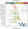 |
Fig. 7 Distribution of first-order MMRs among exoplanet systems in 3+ planet resonant chains as a function of their orbital period. The colour indicates the first-order MMR in which resonant planet pairs are. See Sect. 6 for the selection process. These resonant chains are consistent with a formation by type I migration. As discussed in Sect. 4, low-index (2:1 and 3:2) MMRs tend to belong in uniform resonant chains, while at higher indexes, the inner pair is usually in a higher-index MMR with respect to the outer pair. |
7 Conclusions
Our results provide a more comprehensive view of the capture into resonance in the context of planet formation. We generalised the results from previous numerical studies (Quillen 2006; Ketchum et al. 2011; Ogihara & Kobayashi 2013; Xu et al. 2018) and confirmed some of the trends that were already known, but we also shed light on new behaviours because the parameter space we probed is wide. We staged our experiments in a theoretical context, laid out by the analytical works of Henrard & Lemaitre (1983), Batygin (2015), and Deck & Batygin (2015). Adiabatic resonant capture is possible when the migration timescale through the resonance is assumed to be longer than the resonant libration period. We confirmed that this theoretical framework provides a good description of the mechanism leading to resonant capture, as our results are qualitatively similar to the predictions. However, we showed that the capture for planets undergoing type I migration remains a non-adiabatic mechanism such that the quantitative trends derived from the analytical criterion of Batygin (2015) are not verified. In particular, the eccentricity damping favours the MMR capture and plays a significant role, as highlighted by the results in Sect. 3.2. This, as well as the absence of a dependence of the transition surface density on the planetary masses (in the restricted type I framework), contradicts previous results, such as were obtained by Ogihara & Kobayashi (2013). We conjecture that the use of a more realistic migration prescription (Cresswell & Nelson 2008) is responsible for this discrepancy, as already hinted by Xu et al. (2018). The critical importance of the non-adiabatic mechanisms motivates further theoretical works.
We compared our simulations to the architecture of exoplanet-resonant systems. We find that most of the observed resonant pairs have a low resonant index (k ≤ 2), which is consistent with the capture criteria for planets undergoing migration in a typical protoplanetary disk. This is strong evidence that planetary systems are shaped by the migration. Furthermore, we can study the structure of longer chains as their architecture can be compared to our simulations without knowing the precise conditions during formation. Indeed, resonances within the same system formed under the same conditions. We find that planets composed of low-index resonances are typically in uniform chains, while higher-index resonances are more often in chains of the form k+2:k+1:k, in agreement with ournumerical findings.
Furthermore, as this work can be used to link current architecture and properties of a system to its formation conditions, it is of interest to further build on this study with more detailed models of migration, disk or the inner disk edge. This would take us closer to fully understanding MMR as an important part of planetary evolution.
Acknowledgements
This research has made use of the NASA Exoplanet Archive, which is operated by the California Institute of Technology, under contract with the National Aeronautics and Space Administration under the Exoplanet Exploration Program. This research was made possible by the open-source projects iPython (Perez & Granger 2007), Jupyter (Kluyver et al. 2016), matplotlib (Hunter 2007), numpy (van der Walt et al. 2011), scipy (Virtanen et al. 2020), pandas (McKinney 2010), Rebound(x) (Rein & Liu 2012; Tamayo et al. 2020), and xarray (Hoyer & Hamman 2017). A.J. and A.C.P. acknowledge funding from the European Research Foundation (ERC Consolidator Grant 724687-PLANETESYS), the Knut and Alice Wallenberg Foundation (Wallenberg Scholar Grant 2019.0442), the Swedish Research Council (Project Grant 2018-04867), the Danish National Research Foundation (DNRF Chair Grant DNRF159) and the Göran Gustafsson Foundation.
Appendix A Overstability of the MMR in the case of a more massive outer planet
Planets captured in resonances reach an equilibrium point as eccentricity damping balances the convergent migration (Papaloizou & Szuszkiewicz 2005). However, this equilibrium point can be linearly unstable such that the resonant variable can spiral out of the resonance (Papaloizou & Szuszkiewicz 2010; Xu et al. 2018) by a mechanism called overstability (Deck & Batygin 2015). After the breaking of the resonance, the outer planet continues to migrate towards an inner resonance. Deck & Batygin (2015) found that the resonant fixed point is overstable if the total ratio of the planet-to-star mass is lower than a critical value
 (A.1)
(A.1)
where ζ = m1/m2 is the planet mass ratio, and,  and
and  are related to the eccentricity damping timescales (Deck & Batygin 2015, Eqs. 9 and 14). Using the eccentricity damping expressions from type I migration, we see that
  does not depend on ζ, whereas the sign of
  is roughly proportional to 1 − ζ. It is also straightforward to see that εp,crit is independent of ∑. In particular for ζ ≥ 1 or m1 ≥ m2, εp,crit is negative and the resonance centre is always stable3. In this appendix, we highlight how our result would differ for a more massive outer planet. Similarly to Sect. 3.1, we focus on type I migration by replacing the disk surface density by the rescaled surface density ∑0,gap (Eq. 22). We still highlight the transition to the type II migration regime with a dashed line.
Appendix A.1 Fixed inner planet
We simulated the same system conditions as in Sect. 3.1 with a more massive outer planet, m2 = 2m1 = 2mp, to show how the overstability impacts the final configuration at a lower ratio of planet-to-star mass εp. Figure A.1 shows the resulting 2D grid with varied ∑0,gap and mp. We observe a regime in which the transitions between the resonances do not depend on mp at higher masses, the same as in Fig. 2. Unlike Fig. 2, we also see vertical transitions towards high k for low mp values, most likely due to the overstability of the lower-index resonances. Indeed, a more massive outer planet leads to overstable systems for small mp even for k > 1. According to Deck & Batygin (2015), the threshold value of εp = (m1 + m2)/M* for an overstability increases for all k if the outer planet is more massive, and it generally decreases with increasing k. Moreover, systems close to the boundary to overstability are not in resonance according to Eq. (19). A more detailed study of these system showed that their resonant angles librate significantly, which is consistent with previous studies such as Xu et al. (2018), who showed the continuity between the system escaping the resonance and systems with significant libration. A difference in our results to Deck’s theory is that εp,crit seems to be a decreasing function of the surface density until it reaches the transition surface density observed in the equal-mass case. This more complex pattern was also observed by Xu et al. (2018).
In the case of a more massive inner planet, the results would be qualitatively similar to the equal-mass case detailed in Sect. 3). The overstability mainly occurs for m1 ≲ m2 if the eccentricity-damping timescale is proportional to the planet masses (Deck & Batygin 2015). In the context of the 2:1 MMR, the overstability can be triggered for m1/12 ≲ m2.
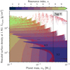 |
Fig. A.1 Final value of the continuous resonance index κ as a function of the rescaled surface density ∑0,gap and mp for systems with mp = m1m2/2. The inner planet is fixed at the inner disk edge, and the initial conditions are otherwise the same as in Fig. 2. The dashed black line is the gap-opening threshold. Except for a few systems, planets with masses below 10−4M⊙ that would otherwise be captured in 2:1 do not stay there due to overstability. |
Appendix A.2 Two migrating planets
We also investigated whether the qualitative behaviour changed when both planets in the simple two-planet system migrate towards the inner disk edge. The initial conditions of this run were the same as in Appendix A.1, but now the inner planet migrated from 0.5 AU and the outer from 0.85 AU. As capture in MMR is only possible for convergent migration, the configuration needs to be such that the outer planet is more massive and thus migrates faster than the inner planet. We used the same mass ratio, m2 = 2m1 = 2mp as in Appendix A.1. As the planet started farther away in the disk, the transition towards the type II regime occurred at a higher mass value.
Figure A.2 shows a 2D grid of final κ values as a function of ∑0,gap and mp. The behaviour of the systems is similar to the previous case. The surface density transitions as well as the over-stable region are similar. Thus, the capture into resonance is not strongly affected by whether both planets are migrating or not, and it only weakly depends on the period of the inner planet at capture, which changes the local surface density and scale height. Figure A.2 also compares well with Fig. 2 in the stable regime. These figures A.2 and A.1 show that overstability exists only for low mp values and is present for higher k MMRs if the outer planet is more massive, as predicted by Deck & Batygin (2015); Xu et al. (2018). Qualitatively, the shape of the boundary is the same as shown in figure 2 in Deck & Batygin (2015) and figure 3 in Xu et al. (2018).
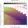 |
Fig. A.2 Same as Fig. A.1, but here, both planets migrate towards the inner disk edge from positions [0.5, 0.85] AU. |
Appendix B Comparing the inner- and outer-planet pairs in the three-planet chain with the two-planet chain
In Sect. 4 we discussed the outcome of the resonant capture in the three-planet case with respect to the two-planet case. We show in Fig. B.1 (Fig. B.2) the difference between the resonant index of the inner (outer) pair of a three-planet system and the resonant index of a two-planet system κ12 − κ2p (κ23 − κ2p) for the same planet mass and disk parameters. As we described in Sect. 4, the inner pair of the three planet system can be pushed into a tighter resonance (higher index) by the capture of the outermost planet. Before the capture of the outer planet, the inner pair behaves in the same way as a two-planet system. For the outer pair, the transitions are noisier, with pairs on both tighter and wider resonances (higher or lower indexes) than their two-planet counterparts.
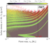 |
Fig. B.1 Difference between the resonant index κ12 of the inner-planet pair in a three-planet system with the index κ2p of a two-planet system for the same planet masses and disk properties (the resonant indexes of the two- and three-planet systems are displayed in Figs. 2 and 4a, respectively). See Fig. 2 for a full description of the setup. As in previous figures, the red dots correspond to systems far from resonance. The dashed black line indicates the threshold for gap opening, 3.3 × 10⁻⁵M⊙. |
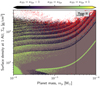 |
Fig. B.2 Same as Fig. B.1 for the difference between the outer-pair resonant index κ23, (shown in Fig. 4b) and the two-planet-system resonant index κ2p. |
References
- Agol, E., Dorn, C., Grimm, S. L., et al. 2021, Planet. Sci. J., 2, 1 [NASA ADS] [CrossRef] [Google Scholar]
- Andrews, S. M., Wilner, D. J., Hughes, A. M., Qi, C., & Dullemond, C. P. 2009, ApJ, 700, 1502 [CrossRef] [Google Scholar]
- Armitage, P. J. 2020, Astrophysics of Planet Formation, 2nd edn. (Cambridge: Cambridge University Press) [CrossRef] [Google Scholar]
- Bai, X.-N., & Stone, J. M. 2011, ApJ, 736, 144 [Google Scholar]
- Baruteau, C., & Papaloizou, J. C. B. 2013, ApJ, 778, 7 [NASA ADS] [CrossRef] [Google Scholar]
- Baruteau, C., Crida, A., Paardekooper, S. J., et al. 2014, in Protostars Planets VI (Tucson: University of Arizona Press), 667 [Google Scholar]
- Batygin, K. 2015, MNRAS, 451, 2589 [NASA ADS] [CrossRef] [Google Scholar]
- Batygin, K., & Adams, F. C. 2017, AJ, 153, 120 [NASA ADS] [CrossRef] [Google Scholar]
- Beauge, C. 1994, Celest. Mech. Dyn. Astron., 60, 225 [NASA ADS] [CrossRef] [Google Scholar]
- Benítez-Llambay, P., Masset, F., Koenigsberger, G., & Szulágyi, J. 2015, Nature, 520, 63 [Google Scholar]
- Bitsch, B., & Kley, W. 2010, A&A, 523, A30 [NASA ADS] [CrossRef] [EDP Sciences] [Google Scholar]
- Bitsch, B., Lambrechts, M., & Johansen, A. 2015, A&A, 582, A112 [NASA ADS] [CrossRef] [EDP Sciences] [Google Scholar]
- Brasser, R., Matsumura, S., Muto, T., & Ida, S. 2018, ApJ, 864, L8 [Google Scholar]
- Charalambous, C., Teyssandier, J., & Libert, A. S. 2022, MNRAS, 514, 3844 [NASA ADS] [CrossRef] [Google Scholar]
- Cresswell, R., & Nelson, R. P. 2006, A&A, 450, 833 [NASA ADS] [CrossRef] [EDP Sciences] [Google Scholar]
- Cresswell, R., & Nelson, R. P. 2008, A&A, 482, 677 [NASA ADS] [CrossRef] [EDP Sciences] [Google Scholar]
- Crida, A., & Morbidelli, A. 2007, MNRAS, 377, 1324 [Google Scholar]
- D’Angelo, G., & Lubow, S. H. 2010, ApJ, 724, 730 [Google Scholar]
- Deck, K. M., & Batygin, K. 2015, ApJ, 810, 119 [Google Scholar]
- Deck, K. M., Payne, M., & Holman, M. J. 2013, ApJ, 774, 129 [Google Scholar]
- Delisle, J.-B., & Laskar, J. 2014, A&A, 570, L7 [NASA ADS] [CrossRef] [EDP Sciences] [Google Scholar]
- Duffell, P. C., & Chiang, E. 2015, ApJ, 812, 94 [NASA ADS] [CrossRef] [Google Scholar]
- Fabrycky, D. C., Ford, E. B., Steffen, J. H., et al. 2012, ApJ, 750, 114 [Google Scholar]
- Fabrycky, D. C., Lissauer, J. J., Ragozzine, D., et al. 2014, ApJ, 790, 146 [Google Scholar]
- Fressin, F., Torres, G., Charbonneau, D., et al. 2013, ApJ, 766, 81 [NASA ADS] [CrossRef] [Google Scholar]
- Friedland, L. 2001, ApJ, 547, L75 [NASA ADS] [CrossRef] [Google Scholar]
- Gladman, B. 1993, Icarus, 106, 247 [Google Scholar]
- Goldreich, P., & Schlichting, H. E. 2014, AJ, 147, 32 [Google Scholar]
- Goldreich, P., & Sciama, D. W. 1965, MNRAS, 130, 159 [NASA ADS] [CrossRef] [Google Scholar]
- Goldreich, P., & Soter, S. 1966, Icarus, 5, 375 [Google Scholar]
- Goldreich, P., & Tremaine, S. 1980, ApJ, 241, 425 [Google Scholar]
- Hadden, S., & Lithwick, Y. 2018, AJ, 156, 95 [NASA ADS] [CrossRef] [Google Scholar]
- Hartmann, L., Calvet, N., Gullbring, E., & D’Alessio, P. 1998, ApJ, 495, 385 [Google Scholar]
- Hasegawa, Y., Okuzumi, S., Flock, M., & Turner, N. J. 2017, ApJ, 845, 31 [NASA ADS] [CrossRef] [Google Scholar]
- Hayashi, C. 1981, Prog. Theor. Phys. Suppl., 70, 35 [Google Scholar]
- Henrard, J. 1982, Celest. Mech., 27, 3 [Google Scholar]
- Henrard, J. 1993, in Dynamics Reported: Expositions in Dynamical Systems, eds. C. K. R. T. Jones, U. Kirchgraber, & H. O. Walther, (Berlin, Heidelberg: Springer), 117 [Google Scholar]
- Henrard, J., & Lemaitre, A. 1983, Celest. Mech., 30, 197 [Google Scholar]
- Hoyer, S., & Hamman, J. 2017, J. Open Res. Softw., 5, 10 [CrossRef] [Google Scholar]
- Huang, S., & Ormel, C. W. 2022, MNRAS, 511, 3814 [NASA ADS] [CrossRef] [Google Scholar]
- Hühn, L.-A., Pichierri, G., Bitsch, B., & Batygin, K. 2021, A&A, 656, A115 [NASA ADS] [CrossRef] [EDP Sciences] [Google Scholar]
- Hunter, J. D. 2007, Comput. Sci. Eng., 9, 90 [NASA ADS] [CrossRef] [Google Scholar]
- Ida, S., Guillot, T., & Morbidelli, A. 2016, A&A, 591, A72 [NASA ADS] [CrossRef] [EDP Sciences] [Google Scholar]
- Izidoro, A., Ogihara, M., Raymond, S. N., et al. 2017, MNRAS, 470, 1750 [Google Scholar]
- Izidoro, A., Bitsch, B., Raymond, S. N., et al. 2021, A&A, 650, A152 [EDP Sciences] [Google Scholar]
- Johansen, A., & Lambrechts, M. 2017, Annu. Rev. Earth Planet. Sci., 45, 359 [Google Scholar]
- Johansen, A., Klahr, H., & Mee, A. J. 2006, MNRAS, 370, L71 [NASA ADS] [Google Scholar]
- Johansen, A., Ida, S., & Brasser, R. 2019, A&A, 622, A202 [NASA ADS] [CrossRef] [EDP Sciences] [Google Scholar]
- Kanagawa, K. D., & Szuszkiewicz, E. 2020, ApJ, 894, 59 [NASA ADS] [CrossRef] [Google Scholar]
- Kanagawa, K. D., Muto, T., Tanaka, H., et al. 2015, ApJ, 806, L15 [NASA ADS] [CrossRef] [Google Scholar]
- Kanagawa, K. D., Tanaka, H., & Szuszkiewicz, E. 2018, ApJ, 861, 140 [Google Scholar]
- Ketchum, J. A., Adams, F. C., & Bloch, A. M. 2011, ApJ, 726, 53 [NASA ADS] [CrossRef] [Google Scholar]
- Kluyver, T., Ragan-Kelley, B., Pérez, F., et al. 2016, in Positioning Power Academic Publishing Play Agents Agendas, eds. F. Loizides & B. Schmidt (Amsterdam: IOS Press), 87 [Google Scholar]
- Lambrechts, M., & Johansen, A. 2012, A&A, 544, A32 [NASA ADS] [CrossRef] [EDP Sciences] [Google Scholar]
- Lambrechts, M., Morbidelli, A., Jacobson, S. A., et al. 2019, A&A, 627, A83 [NASA ADS] [CrossRef] [EDP Sciences] [Google Scholar]
- Laskar, J., & Robutel, P. 1995, Celest. Mech. Dyn. Astron., 62, 193 [Google Scholar]
- Lega, E., Nelson, R. P., Morbidelli, A., et al. 2021, A&A, 646, A166 [NASA ADS] [CrossRef] [EDP Sciences] [Google Scholar]
- Leleu, A., Alibert, Y., Hara, N. C., et al. 2021, A&A, 649, A26 [NASA ADS] [CrossRef] [EDP Sciences] [Google Scholar]
- Lemaitre, A. 1984, Celest. Mech., 32, 109 [NASA ADS] [CrossRef] [Google Scholar]
- Lin, D. N. C., & Papaloizou, J. 1979, MNRAS, 186, 799 [Google Scholar]
- Lin, D. N. C., & Papaloizou, J. C. B. 1993, in Protostars Planets III (Tucson: University of Arizona Press), 749 [Google Scholar]
- Manara, C. F., Rosotti, G., Testi, L., et al. 2016, A&A, 591, L3 [NASA ADS] [CrossRef] [EDP Sciences] [Google Scholar]
- Manara, C. F., Ansdell, M., Rosotti, G. P., et al. 2022, ArXiv eprints [arXiv:2203.09930] [Google Scholar]
- Marchal, C., & Bozis, G. 1982, Celest. Mech. Dyn. Astron., 26, 311 [NASA ADS] [CrossRef] [Google Scholar]
- Masset, F. S., Morbidelli, A., Crida, A., & Ferreira, J. 2006, ApJ, 642, 478 [Google Scholar]
- Matsumoto, Y., & Ogihara, M. 2020, ApJ, 893, 43 [Google Scholar]
- Matsumoto, Y., Nagasawa, M., & Ida, S. 2012, Icarus, 221, 624 [Google Scholar]
- McKinney, W. 2010, in Proceedings of 9th Python Science Conference, ed. S. van der Walt & Jarrod Millman, 51 [Google Scholar]
- McNally, C. P., Nelson, R. P., Paardekooper, S.-J., Benitez-Llambay, P., & Gressel, O. 2020, MNRAS, 493, 4382 [NASA ADS] [CrossRef] [Google Scholar]
- Millholland, S., & Laughlin, G. 2019, Nat. Astron., 3, 424 [Google Scholar]
- Murray, C. D., & Dermott, S. F. 1999, Solar System Dynamics (Cambridge: Cambridge University Press) [Google Scholar]
- Mustill, A. J., & Wyatt, M. C. 2011, MNRAS, 413, 554 [NASA ADS] [CrossRef] [Google Scholar]
- Ogihara, M., & Kobayashi, H. 2013, ApJ, 775, 34 [Google Scholar]
- Paardekooper, S.-J., Baruteau, C., Crida, A., & Kley, W. 2010, MNRAS, 401, 1950 [NASA ADS] [CrossRef] [Google Scholar]
- Paardekooper, S.-J., Baruteau, C., & Kley, W. 2011, MNRAS, 410, 293 [NASA ADS] [CrossRef] [Google Scholar]
- Papaloizou, J. C. B., & Szuszkiewicz, E. 2005, MNRAS, 363, 153 [Google Scholar]
- Papaloizou, J. C. B., & Szuszkiewicz, E. 2010, EAS Pub. Ser., 42, 333 [NASA ADS] [CrossRef] [EDP Sciences] [Google Scholar]
- Peale, S. J. 1976, Annu. Rev. Astron. Astrophys., 14, 215 [CrossRef] [Google Scholar]
- Perez, F., & Granger, B. E. 2007, Comput. Sci. Eng., 9, 21 [Google Scholar]
- Petigura, E. A., Marcy, G. W., Winn, J. N., et al. 2018, AJ, 155, 89 [Google Scholar]
- Petit, A. C., Laskar, J., & Boué, G. 2017, A&A, 607, A35 [NASA ADS] [CrossRef] [EDP Sciences] [Google Scholar]
- Petit, A. C., Laskar, J., & Boué, G. 2018, A&A, 617, A93 [NASA ADS] [CrossRef] [EDP Sciences] [Google Scholar]
- Petit, A. C., Petigura, E. A., Davies, M. B., & Johansen, A. 2020a, MNRAS, 496, 3101 [NASA ADS] [CrossRef] [Google Scholar]
- Petit, A. C., Pichierri, G., Davies, M. B., & Johansen, A. 2020b, A&A, 641, A176 [NASA ADS] [CrossRef] [EDP Sciences] [Google Scholar]
- Pichierri, G., & Morbidelli, A. 2020, MNRAS, 494, 4950 [Google Scholar]
- Pichierri, G., Morbidelli, A., & Crida, A. 2018, Celest. Mech. Dyn. Astron., 130, 54 [Google Scholar]
- Pichierri, G., Batygin, K., & Morbidelli, A. 2019, A&A, 625, A7 [NASA ADS] [CrossRef] [EDP Sciences] [Google Scholar]
- Quillen, A. C. 2006, MNRAS, 365, 1367 [Google Scholar]
- Raymond, S. N., Izidoro, A., Bolmont, E., et al. 2021, Nat. Astron., 6, 80 [NASA ADS] [CrossRef] [Google Scholar]
- Rein, H., & Liu, S.-F. 2012, A&A, 537, A128 [NASA ADS] [CrossRef] [EDP Sciences] [Google Scholar]
- Rein, H., & Tamayo, D. 2015, MNRAS, 452, 376 [Google Scholar]
- Rivera, E. J., Laughlin, G., Butler, R. P., et al. 2010, ApJ, 719, 890 [Google Scholar]
- Sessin, W., & Ferraz-Mello, S. 1984, Celest. Mech., 32, 307 [NASA ADS] [CrossRef] [Google Scholar]
- Shakura, N. I., & Sunyaev, R. A. 1973, A&A, 24, 337 [NASA ADS] [Google Scholar]
- Tabone, B., Rosotti, G. R., Lodato, G., et al. 2022, MNRAS, 512, L74 [NASA ADS] [CrossRef] [Google Scholar]
- Tamayo, D., Rein, H., Shi, P., & Hernandez, D. M. 2020, MNRAS, 491, 2885 [NASA ADS] [CrossRef] [Google Scholar]
- Tanaka, H., & Ward, W. R. 2004, ApJ, 602, 388 [Google Scholar]
- Tanaka, H., Takeuchi, T., & Ward, W. R. 2002, ApJ, 565, 1257 [Google Scholar]
- Tazzari, M., Testi, L., Natta, A., et al. 2017, Astron. Amp. Astrophys., 606, A88 [NASA ADS] [CrossRef] [EDP Sciences] [Google Scholar]
- Testi, L., Natta, A., Manara, C. F., et al. 2022, A&A, 663, A98 [NASA ADS] [CrossRef] [EDP Sciences] [Google Scholar]
- Teyssandier, J., & Libert, A.-S. 2020, Astron. Amp. Astrophys. 643, A11 [NASA ADS] [CrossRef] [EDP Sciences] [Google Scholar]
- van der Walt, S., Colbert, S. C., & Varoquaux, G. 2011, Comput. Sci. Eng., 13, 22 [Google Scholar]
- Virtanen, P., Gommers, R., Oliphant, T. E., et al. 2020, Nat. Methods, 17, 261 [Google Scholar]
- Ward, W. R. 1997, Icarus, 126, 261 [Google Scholar]
- Weiss, L. M., Marcy, G. W., Petigura, E. A., et al. 2018, AJ, 155, 48 [Google Scholar]
- Wisdom, J. 1980, AJ, 85, 1122 [NASA ADS] [CrossRef] [Google Scholar]
- Xu, W., Lai, D., & Morbidelli, A. 2018, MNRAS, 481, 1538 [Google Scholar]
- Yoder, C. F. 1979, Celest. Mech., 19, 3 [NASA ADS] [CrossRef] [Google Scholar]
- Zhu, W., & Dong, S. 2021, Annu. Rev. Astron. Astrophys., 59, 291 [CrossRef] [Google Scholar]
The discussion is slightly different for the 2:1 MMR; see Deck & Batygin (2015).
All Figures
|
Fig. 1 Final continuous resonance index k (Eq. (18)) of two equal-mass planets as a function of the surface density Σ0 at 1 AU and the planet mass mp. The inner planet is fixed at the inner disk edge (0.1 AU), while the outer planet migrates from 0.2 AU. Systems that do not satisfy 0 < Δ < 0.03 are considered not in resonance and are plotted in red. Hill-unstable systems are removed and are plotted in white. The dashed line indicates the transition mass (Eq. (14)) to the regime of type II migration. The accretion rate displayed on the right axis is computed from Eq. (4) assuming a viscous parameter α = 10−2. |
| In the text | |
|
Fig. 2 Final continuous resonance index κ (Eq. (18)) of two equal-mass planets as a function of the rescaled surface density Σ0,gap (Eq. (22)) and the planet mass mp. Using the rescaled surface density allows highlighting the dynamically relevant quantity for the resonant capture. |
| In the text | |
|
Fig. 3 Continuous resonance index κ for a pair of 10−5 M⊙ equal-mass planets as a function of the rescaled surface density Σ0,gap (Eq. (22)) and the disk aspect ratio h0. The green line verifies Σ0 ∝ h2, corresponding to a constant migration timescale. The yellow line is an example of the fitted |
| In the text | |
|
Fig. 4 Continuous resonant indexes κ12 (a) and κ23 (b) of the inner and outer pair of planets as a function of mp and Σ0 for three equal-mass planet systems. The innermost planet is initialised at the inner disk edge, while the other two planets migrate from 0.2 and 0.3 AU, respectively. The initial conditions are otherwise identical to the first run presented in Fig. 2. The dashed black line indicates the gap-opening threshold at 3.3 × 10⁻⁵ M⊙. |
| In the text | |
|
Fig. 5 Difference κ12 − κ23 of the inner and outer pair continuous resonant indexes as a function of the planet mass mp and the surface density Σ0. As in previous figures, the red dots correspond to systems far from resonance, and the dashed black line corresponds to the gap-opening threshold (3.3 × 10⁻⁵M⊙). |
| In the text | |
|
Fig. 6 Transition surface densities |
| In the text | |
|
Fig. 7 Distribution of first-order MMRs among exoplanet systems in 3+ planet resonant chains as a function of their orbital period. The colour indicates the first-order MMR in which resonant planet pairs are. See Sect. 6 for the selection process. These resonant chains are consistent with a formation by type I migration. As discussed in Sect. 4, low-index (2:1 and 3:2) MMRs tend to belong in uniform resonant chains, while at higher indexes, the inner pair is usually in a higher-index MMR with respect to the outer pair. |
| In the text | |
|
Fig. A.1 Final value of the continuous resonance index κ as a function of the rescaled surface density ∑0,gap and mp for systems with mp = m1m2/2. The inner planet is fixed at the inner disk edge, and the initial conditions are otherwise the same as in Fig. 2. The dashed black line is the gap-opening threshold. Except for a few systems, planets with masses below 10−4M⊙ that would otherwise be captured in 2:1 do not stay there due to overstability. |
| In the text | |
|
Fig. A.2 Same as Fig. A.1, but here, both planets migrate towards the inner disk edge from positions [0.5, 0.85] AU. |
| In the text | |
|
Fig. B.1 Difference between the resonant index κ12 of the inner-planet pair in a three-planet system with the index κ2p of a two-planet system for the same planet masses and disk properties (the resonant indexes of the two- and three-planet systems are displayed in Figs. 2 and 4a, respectively). See Fig. 2 for a full description of the setup. As in previous figures, the red dots correspond to systems far from resonance. The dashed black line indicates the threshold for gap opening, 3.3 × 10⁻⁵M⊙. |
| In the text | |
|
Fig. B.2 Same as Fig. B.1 for the difference between the outer-pair resonant index κ23, (shown in Fig. 4b) and the two-planet-system resonant index κ2p. |
| In the text | |
Current usage metrics show cumulative count of Article Views (full-text article views including HTML views, PDF and ePub downloads, according to the available data) and Abstracts Views on Vision4Press platform.
Data correspond to usage on the plateform after 2015. The current usage metrics is available 48-96 hours after online publication and is updated daily on week days.
Initial download of the metrics may take a while.