| Issue |
A&A
Volume 669, January 2023
|
|
|---|---|---|
| Article Number | A17 | |
| Number of page(s) | 9 | |
| Section | Stellar atmospheres | |
| DOI | https://doi.org/10.1051/0004-6361/202244305 | |
| Published online | 23 December 2022 | |
First r-process enhanced star confirmed as a member of the Galactic bulge
1
Lund Observatory, Department of Astronomy and Theoretical Physics, Lund University,
Box 43,
22100
Lund, Sweden
e-mail: This email address is being protected from spambots. You need JavaScript enabled to view it.
2
Department of Physics and Astronomy, ICLA,
430 Portola Plaza,
Box 951547,
Los Angeles, CA
90095-1547, USA
3
Université Côte-d’Azur, Observatoire de la Côte d'Azur, Laboratoire Lagrange, CNRS,
Blvd de l’Observatoire,
06304
Nice, France
4
Materials Science and Applied Mathematics, Malmö University,
205 06
Malmö, Sweden
5
Department of Astronomy, School of Science, The University of Tokyo,
7-3-1 Hongo, Bunkyo-ku,
Tokyo
113-0033, Japan
Received:
20
June
2022
Accepted:
10
October
2022
Abstract
Aims. Stars with strong enhancements of r-process elements are rare and tend to be metal-poor, generally with [Fe/H] < −2 dex, and located in the halo. In this work, we aim to investigate a candidate r-process enriched bulge star with a relatively high metallicity of [Fe/H] ~ − 0.65 dex and to compare it with a previously published r-rich candidate star in the bulge.
Methods. We reconsidered the abundance analysis of a high-resolution optical spectrum of the red-giant star 2MASS J18082459-2548444 and determined its europium (Eu) and molybdenum (Mo) abundance, using stellar parameters from five different previous studies. Applying 2MASS photometry, Gaia astrometry, and kinematics, we estimated the distance, orbits, and population membership of 2MASS J18082459-2548444 and a previously reported r-enriched star 2MASS J18174532-3353235.
Results. We find that 2MASS J18082459-2548444 is a relatively metal-rich, enriched r-process star that is enhanced in Eu and Mo, but not substantially enhanced in s-process elements. There is a high probability that it has a Galactic bulge membership, based on its distance and orbit. We find that both stars show r-process enhancement with elevated [Eu/Fe]-values, even though 2MASS J18174532-3353235 is 1 dex lower in metallicity. Additionally, we find that the plausible origins of 2MASS J18174532-3353235 to be either that of the halo or the thick disc.
Conclusions. We conclude that 2MASS J18082459-2548444 represents the first example of a confirmed r-process enhanced star confined to the inner bulge. We assume it is possibly a relic from a period of enrichment associated with the formation of the bar.
Key words: stars: abundances / stars: chemically peculiar / Galaxy: bulge / Galaxy: evolution
© The Authors 2022
 Open Access article, published by EDP Sciences, under the terms of the Creative Commons Attribution License (https://creativecommons.org/licenses/by/4.0), which permits unrestricted use, distribution, and reproduction in any medium, provided the original work is properly cited.
This article is published in open access under the Subscribe-to-Open model. This email address is being protected from spambots. You need JavaScript enabled to view it. to support open access publication.
1 Introduction
The composition of stars presents a record of the formation and chemical enrichment of the Milky Way. Stars form from molecular clouds and can potentially carry a chemical fingerprint of their birth cloud that may include pollution from earlier events. The Galactic interstellar medium is chemically enriched over time, through nucleosynthetic processes occurring either in stars or in explosive environment such as supernovae (SNe) and neutron star mergers.
The Galactic bulge is of great interest because of its age and high metallicity, which are consistent with early, rapid enrichment. The modern era of study gave observations of high iron abundance and α-enhancements (Rich 1988; McWilliam & Rich 1994) paired with old age (Ortolani et al. 1995) have substantiated this picture of rapid enrichment via Type II SNe (Matteucci & Brocato 1990). The actual picture may be more nuanced. Deep studies of the main sequence in fields imaged by the ESA/NASA Hubble Space Telescope largely support a predominant older age (Clarkson et al. 2008; Renzini et al. 2018), while Bensby et al. (2017) have argued for a far greater dispersion in age, based on the analysis of microlensed bulge dwarfs. A recent study by Joyce et al. (2022) confirms that the most metal-rich stars may be younger than 10 Gyr, with a 5 Gyr age dispersion.
Stars with [Fe/H] > −0.5 dex are predominantly in a bar (Ness et al. 2012, 2013) that appears to have formed via the buckling of a pre-existing disc (Shen et al. 2010; Di Matteo et al. 2014). Overall, in the present day, a tension is apparent between seemingly robust evidence for early rapid enrichment from analyses of color-magnitude diagrams and luminosity functions, with the study of the microlensed dwarfs providing a counterpoint of possibly extended formation. The progressive flattening of the metal-rich population (Johnson et al. 2020) offers some support for the extended formation scenario.
This tension between evidence of early enrichment in the bulge versus a potentially extended formation history for the most metal-rich bulge populations is an intriguing area or research where still much can be learnt. One characteristic of the ancient Galactic halo is the presence of neutron-capture (Burbidge et al. 1957) enhanced stars, especially those with high amount of r-process elements. The discovery of a bulge or inner halo candidate displaying the full r-process pattern (Johnson et al. 2013) raises the possibility that such stars also formed early in the history of the bulge or inner halo.
These types of r-enhanced stars remain rare, but are of sufficient interest that they have been catalogued and studied across Galactic populations, with more than 300 known at this time (see the R-process Alliance, Holmbeck et al. 2020).
Whilst the origins of such enhancements remain an open matter of discussion to date, and it is possible that the primary source has changed over time (Sneden et al. 2008), they are proposed to offer clear signatures of r-process events. Such events could be neutron star mergers (NSM, Matteucci et al. 2014) and/or magneto-rotational driven SNe (MRSNe, Nishimura et al. 2006; Kobayashi et al. 2020) which can provide the neutron-rich conditions that favour the nucleogenesis of these heavy elements.
In general, stars showing r-process enhancements are metal poor, with [Fe/H] < −2 dex (McWilliam et al. 1995; Sneden et al. 2003, 2008; Holmbeck et al. 2020), appearing in the Milky Way halo and in dwarf galaxies (Hirai et al. 2015; Matsuno et al. 2021; Jeon et al. 2021). These are classified into two groups, r-I and r-II, depending on the level of r-process enrichment. The discrepancy of r-I and r-II stars has been given by 0.3 < [Eu/Fe] ≤ 1.0 dex and [Eu/Fe] > 1.0 dex, respectively, with [Ba/Eu] < 0 dex for the r-II stars (Christlieb et al. 2004). In the R-process Alliance, they listed 232 r-I and 72 r-II stars, whilst proposing a new demarcation between these two groups at [Eu/Fe] = 0.7 dex (Holmbeck et al. 2020). As the astrophysical site(s) of the r-process remains a matter of vigorous debate (see e.g. Côté et al. 2019), it continues to be important to document such stars in a range of stellar populations as their presence potentially gives insight into the early enrichment history of a population.
One interesting set of spectra was first used in Zoccali et al. (2006) and later reanalysed in several subsequent studies (Lecureur et al. 2007; Ryde et al. 2010; Van der Swaelmen et al. 2016; Jönsson et al. 2017b; Lomaeva et al. 2019; Forsberg et al. 2019, 2022). A star found in the set, the K-giant 2MASS J18082459-2548444 (hereafter, the Z06-star), has recently been shown to be high in [Eu/Fe] (Van der Swaelmen et al. 2016; Forsberg et al. 2019) and [Mo/Fe] (Forsberg et al. 2022). At [Fe/H] ~ − 0.65 dex (Lecureur et al. 2007; Zoccali et al. 2008; Ryde et al. 2010; Johnson et al. 2014; Jönsson et al. 2017b), this star is remarkably high in metallicity for a potentially r-process enhanced star. Whilst at present we focus our reporting only on this star, the discovery of it makes emphatic the importance of searching for other stars with unusual enhancements of heavy elements that are also found in the Galactic bulge.
Indeed, Johnson et al. (2013) published the first r-enriched candidate in the Galactic bulge, 2MASS J18174532-3353235, located at (l, b) = (−1, −8)°. The star is reported to have a relatively high metallicity (relative the halo r-enhanced population) of [Fe/H] = −1.67 dex and an r-enrichment as traced by europium of [Eu/Fe] = 1.0 dex and molybdenum of [Mo/Fe] = 0.72 dex. It should be noted that Johnson et al. (2013) did not rule out a halo origin for 2MASS J18174532-3353235 (hereafter, the J13-star) and noted that with more precise proper motions, the kinematics of the star would be constrained with a greater certainty.
In this work, we re-analyse the optical spectrum of the Z06-star, as described in Sect. 2. We use the stellar parameters from the earlier studies (Zoccali et al. 2006; Lecureur et al. 2007; Ryde et al. 2010; Van der Swaelmen et al. 2016; Jönsson et al. 2017b) to determine the abundances of the r-process elements europium and molybdenum, as described in Sect. 3. We compare the results with studies from Forsberg et al. (2019, 2022). In Sect. 4, we investigate the bulge membership of the two r-enhanced stars, the Z06-star, 2MASS J18082459-2548444, and the J13-star, 2MASS J18174532-3353235. With the data from Gaia Early Data Release 3 (Gaia EDR3, Gaia Collaboration 2021), we now have access to a highly precise value for the proper motion of these stars, allowing us to calculate their orbits.
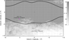 |
Fig. 1 Map of the Galactic bulge, showing the position of the Z06-star, 2MASS J18082459-2548444 (magenta), and the J13-star, 2MASS J18174532-3353235 (teal), presented in this work. The dust extinction towards the bulge is taken from Gonzalez et al. (2011, 2012) and scaled to optical extinction (Cardelli et al. 1989). The scale saturates at AV = 2, setting the upper limit. We also plot the COBE/DIRBE outlines of the Galactic bulge (Weiland et al. 1994). |
2 Observational data
The spectrum of the Z06-star is part of the Zoccali et al. (2006) data set and has been observed with the FLAMES-UVES (R ~ 47 000) at the European Southern Observatory’s Very Large Telescope (ESO’s VLT). The spectral wavelength is limited to 5800–6800 Å. The star is located at (l, b) = (5.2°, −2.8°), placing it in the line of sight within the bulge as outlined from COBE/DIRBE (Weiland et al. 1994), as seen in Fig. 1.
The stellar parameters of the Z06-star were determined in Lecureur et al. (2007); Zoccali et al. (2008); Ryde et al. (2010); Johnson et al. (2014); Jönsson et al. (2017b). We provide more details in Table 1. With an effective temperature of ~4400 K and log(g) of ~ 1.75, it is a typical red-giant star. With the combined works of Lecureur et al. (2007); Ryde et al. (2010); Johnson et al. (2014); Van der Swaelmen et al. (2016); Jönsson et al. (2017b); Lomaeva et al. (2019); Forsberg et al. (2019, 2022), the known chemical fingerprint of the Z06-star consists of 21 abundances (see Table 2).
The J13-star, placed at (l, b) = (1°, −8°), is also marked in Fig. 1 and is found within the bulge Plaut field. The spectrum of the J13-star, analysed in Johnson et al. (2013), has been observed with the Magellan Inamori Kyocera Echelle (MIKE) spectrograph on the 6.5 m Magellan Clay telescope (R ~ 30000).
3 Analysis of the spectrum
In this section, we give a brief discussion of the analysis of the spectrum of the Z06-star, where we follow the methodology as outlined in the Jönsson-series (Jönsson et al. 2017a,b; Lomaeva et al. 2019; Forsberg et al. 2019, 2022). We re-determine the Mo and Eu abundances using the stellar parameters presented in Lecureur et al. (2007); Zoccali et al. (2008); Ryde et al. (2010); Johnson et al. (2014) to confirm the high abundances determined in previous papers. We refer to these papers for a more detailed description of the stellar parameters and details of the elemental abundance determination for the other elements presented in Table 2.
The analysis of the spectra is done using the tool Spectroscopy Made Easy (SME, version 554 Valenti & Piskunov 1996; Piskunov & Valenti 2017). This tool uses a grid of MARCS models1 (Gustafsson et al. 2008), with spherical symmetry for log(g) < 3.5, which is applicable to the Z06-star and the bulge stars analysed in the Jönsson-series. The atomic data comes from the Gaia-ESO line list version 6 (Heiter et al. 2021).
In order for SME to produce a synthetic spectrum, it requires a line list, model atmospheres, and defined spectral segments, as well as spectral line and continuum masks. The masks are defined manually around the spectral line of interest, which in Jönsson et al. (2017a,b); Lomaeva et al. (2019); Forsberg et al. (2019, 2022) was shown to be crucial for obtaining the high-precision abundances they report.
Comparison of the stellar parameters (Cols. 2-5) for the Z06-star from five different spectroscopic studies (Col. 1).
Determined absolute abundances A(X) and solar- and metallicity-normalised abundances [X/Fe] of the Z06-star.
3.1 Europium
For europium (Eu, Z = 63), we used the Eu II 6645 Å spectral line for the abundance determination, with the atomic data from the Gaia-ESO (GES) line list version 6 (Heiter et al. 2021). They classified the 6645 Å line as ‘yes/uncertain’, indicating that the log(gf)-value was of high quality, however that there could be some uncertain blends in the line. They recommended the line to be used only for giant stars with high S/N spectra, which is the case for the Zoccali et al. (2006) – spectrum of the Z06-star used here. Europium has both hyperfine structure and two stable isotopes in the Sun. The hyperfine splitting is included in the GES line list, whereas the isotopic shift cannot be resolved and is not included.
This line has been used with the same analysis as described here to determine the Eu abundance for close to 300 disc K-giants in Forsberg et al. (2019). Their abundance trend is tightly correlated with [Fe/H], giving confidence in the quality of our analysis presented here. However, we do note that the [Eu/Fe] abundances seems to be systematically too high in the disc stars in Forsberg et al. (2019), which might be explained by the possible systematic uncertainty in their log(g) as reported in Jönsson et al. (2017a,b) when compared to Gaia Benchmark stars (in Jofré et al. 2014, 2015; Heiter et al. 2015). Therefore, we systematically lowered the overall disc abundances with 0.10 dex, such that the thin disc trend passes through the Solar value, as can be seen in Fig. 2. For the same reasons, the [La,Ce/Fe] values are also systematically lowered, as shown in Table 2.
Nonetheless, the [Eu/Fe] value for the Z06-starfrom their study remains high, which is confirmed by determining the abundance using the Lecureur et al. (2007); Zoccali et al. (2008); Ryde et al. (2010); Johnson et al. (2014) stellar parameters as well, which do not report any systematics in their parameters, indicating the Eu-content to indeed be high in the Z06-star.
3.2 Molybdenum
For molybdenum (Mo, Z = 42), we used the Mo I 6030 Å spectral line for the abundance determination, which is very weak in dwarf stars but usable in giant stars (Forsberg et al. 2022). In Heiter et al. (2021) the line is reported to be Yes/Yes, having well-known atomic data and being unblended. Mo does not have hyperfine structure, but it has seven stable isotopes in the Sun. Similarly to Eu, this isotopic splitting is not included in the linelist and we determine the abundance using the five sets of stellar parameters given in Table 1. The manually defined line- and continuum masks can be seen in Fig. 3. Both the spectrum of the Z06-star and the synthetic spectrum can be seen in Fig. 4, with a ±0.1 dex uncertainty.
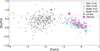 |
Fig. 2 [Eu/Fe] over [Fe/H] for the Z06-star (magenta star) and the J13-star (teal diamond). For reference, we plot the bulge (magenta circles) and disc stars (grey squares) from Forsberg et al. (2019) as well as the bulge stars from Johnson et al. (2012). The abundances of the halo stars come from the r-process alliance sample (dark grey triangles Holmbeck et al. 2020). The orange line indicates the ‘r-II’ limit as defined in the r-process alliance (Holmbeck et al. 2020). We note that the abundances from Forsberg et al. (2019) have been systematically lowered with 0.10 dex, as described in Sect. 3.1. |
4 Bulge membership
A majority of the r-process enriched stars are metal-poor, [Fe/H] ≤ −1.5 dex, and confined to the Galactic halo (Holmbeck et al. 2020). In order to investigate whether the Z06-star and the J13-star are likely to be confined to the Galactic bulge or visiting halo-stars, we estimated their line-of-sight distances and, using their proper motions (from Gaia EDR3, Gaia Collaboration 2016, 2021), we estimated their orbits using galpy (Bovy 2015). The line-of-sight positions of both stars can be seen in Fig. 1, where the Z06-star is closer to the Galactic plane, compared to the J13-star.
4.1 Distance estimates
We calculated the spectrophotometric distances for the two stars for which we incorporated the stellar properties Teff, log(g), [Fe/H], and the 2MASS JHKs photometry into the spectrophotometry method described in Rojas-Arriagada et al. (2017). For the stellar parameters, we used the Jönsson et al. (2017b) parameters for the Z06-star, and Johnson et al. (2013) parameters for the J13-star. Each parameter point in the parameter space Teff, log(g), [Fe/H] is compared to a set of theoretical isochrones for each star. We use the PARSEC isochrones (Bressan et al. 2012; Marigo et al. 2017) spanning ages from 1 to 13 Gyr in steps of 1 Gyr and metallicities from −2.2 to +0.5 in steps of 0.1 dex. We note that the PARSEC isochrones do not take α-elements into account.
A number of extra multiplicative weights are defined to account for the evolutionary speed of the points along the isochrones and for the initial mass function. Using these weights, the most likely absolute magnitudes (MJ, MH, MKs) of the observed stars can be computed as the weighted mean or median of the theoretical values of the whole set of isochrone points. The computed absolute magnitudes are then compared to the observed photometry, allowing us to estimate the line-of-sight reddening and distance modulus. These distances were extensively tested and used within the APOGEE survey (Majewski et al. 2017; see e.g. Rojas-Arriagada et al. 2020; Zasowski et al. 2019).
For the Z06-star we derive a heliocentric distance of 7.2 ± 0.3kpc and for the J13-star 11.8 ± 1.0 kpc. The uncertainties for the distances are estimated using the reported uncertainties of the photometry and stellar parameters. These distances indicate that the Z06-star belongs to the Galactic bulge, while the large distance of the J13-star suggests, together with its low metallicity of [Fe/H] = −1.69 dex, that it originates from either the Galactic halo or thick disc. This hypothesis was indeed already suggested by Johnson et al. (2013).
In addition, we calculated the distances using the Gaia DR3 photometry in the G-band (Kordopatis et al. 2022) for these two stars in order to check the consistency. A distance of 7.4 ± 1.0 kpc has been obtained for the Z06-star and of 12.2 ± 1.5 kpc for the J13-star, respectively. This strengthen our argument that indeed the J13-star is a visiting halo or inner halo or a thick disc star, while the Z06-star belongs to the Galactic bulge.
4.2 Modelling of orbits
To further investigate the bulge membership, we explored possible orbits of the stars using GalPy (Bovy 2015). We adopted the Milky Way like MWPotential2014-potential (Bovy 2015), which includes an axisymmetric disc, a halo, and a spherical bulge. To that, we added the Dehnen (2000)-bar potential (which in GalPy has been generalised to 3D following Monari et al. 2016).
We integrate the orbits up to 10 Gyr for both stars, using positions in RA+Dec; proper motions (Gaia Collaboration 2021); distances as derived above; and radial velocities determined in Johnson et al. (2013); Jönsson et al. (2017b). We also calculated the orbits using the uncertainties for distances and proper motions to check whether the orbits remain similar. The data used can be seen in Table 3. As a sanity check, we also calculated the orbits using the AGAMA code (Vasiliev 2019), where we implement a combined MWPotential2014 and Launhardt et al. (2002) – inner bulge potential. The code gives similar results as the ones presented for GalPy.
5 Results and discussion
We present the abundances of the Z06-star and compare with both the J13-star and the overall bulge sample as determined in our series of papers. We show and discuss the orbits as well as the distances, and we consider the implications for the formation history of the bulge.
5.1 Abundances
We re-analysed the spectrum of the Z06-star and determine both the [Eu/Fe] and [Mo/Fe] abundance using the stellar parameters reported in Lecureur et al. (2007); Zoccali et al. (2008); Ryde et al. (2010); Johnson et al. (2014); Jönsson et al. (2017b), which can be seen in Table 1.
From these, we find that the Z06-star has a mean [Eu/Fe] = 0.80 dex, based on the five different stellar parameter determinations, pointing at the Eu-content being high in the Z06-star, independently on the stellar parameters. All of the values are [Eu/Fe] ≥ +0.74 dex, which classifies it as a, relatively metal-rich, r-II star (following the classification in the R-process Alliance, Holmbeck et al. 2020). In Fig. 2 we show [Eu/Fe] vs. [Fe/H] for the bulge stars in Forsberg et al. (2019) and Johnson et al. (2012), which both include the Z06-star and the J13-star, respectively. We also plot the typical local disc abundances (Forsberg et al. 2019) and stars from the R-process Alliance (Holmbeck et al. 2020). We note that even though the [Eu/Fe]-abundances from Forsberg et al. (2019) has been systematically lowered with 0.10 dex, as described in Sect. 3.1, both the Z06-star and the J13-star lie above the Holmbeck et al. (2020) – classification boundary for an r-II star, and are high in [Eu/Fe] as compared to the bulge samples.
The [Mo/Fe] abundance for the Z06-star is high with 0.62 dex from the Forsberg et al. (2022) study, and an average of 0.66 dex when determined using the five different stellar parameter studies (Table 1). In Fig. 5, we show the [Mo/Fe] abundances for the local disc and the bulge (Forsberg et al. 2022), including the Z06-star. We have also added the J13-star and molybdenum abundances from disc and halo studies (Peterson 2013; Hansen et al. 2014; Roederer et al. 2014; Mishenina et al. 2013).
In order to make a comparison amongst the stars, in Fig. 6, we compared their [X/Fe] in with the overall bulge abundances as measured from the Jönsson-series (Johnson et al. 2017b; Lomaeva et al. 2019; Forsberg et al. 2019, 2022). We see that both the Z06-star and the J13-star are enhanced in [Mo/Fe] and [Eu/Fe]. Additionally, both stars are on the higher side in the s-process elements [Zr,La/Fe]. This pattern of high abundance in heavier elements is similar to that of the prototypical r-process enhanced metal-poor halo stars BD +17°3248 (Cowan et al. 2002), CS 22892-052 (Sneden et al. 2003) and HD 222925 (Roederer et al. 2022).
Europium has a close to pure r-process origin with 96% r-process contribution at solar metallicites. Molybdenum has a more complex cosmic origin, as is composed of seven stable isotopes, with either an s-, r-, and p-process origin, or a combination of them. The r-process contribution varies a bit in the literature, from 27% to 36% at solar metallicities (Prantzos et al. 2020; Bisterzo et al. 2014, respectively). Mo has a roughly 25% origin from the p-process, a process which have several suggested cosmic sites and mechanisms behind it. It is likely to take place in proton-dense and/or explosive environments, which points toward fast timescales, such as core-collapse SNe, events linked to SNe type la, or mass-accreting neutron stars (see e.g. Rauscher et al. 2013; Forsberg et al. 2022). At the low metallicites of −0.65 and −1.67 dex for the stars, the s-process, taking place in AGB-stars, is less likely to contribute to the production the Mo (Karakas & Lattanzio 2014; Cescutti et al. 2015; Cescutti & Matteucci 2022). As such, at low metallicities Mo is effectively an r-process and p-process element. The same applies to Zr and La, which at lower metallicities have a dominating production from the r-process.
To decipher if the high neutron-capture abundances have an r- or s-process origin, we considered the [s/r]-ratio. Both the Z06-star and the J13-star have rather low [La/Eu]-ratio of −0.36 and −0.44 dex, respectively. Additionally, the [Ce/Eu]-ratio2 is −0.56 and −0.62 dex, respectively, for the Z06-star and J13-star. This supports a significant contribution from the r-process in the enrichment of these two stars, and less significant contribution from the s-process (which is, indeed, the case for many bulge stars; see e.g. McWilliam 2016).
Although many stars with high r-process enhancements are known (Cowan et al. 2002; Sneden et al. 2003, 2008; Christlieb et al. 2004; Holmbeck et al. 2020), it is rare to find one at the comparatively high metallicities of the J13-star and the Z06-star. It should be noted that the metallicity distribution in the bulge varies with latitude, where the metallicity is higher towards the plane (see e.g. Johnson et al. 2020). As such, the Z06-star is metal-poor relative to its neighbouring stars. The same applies for the J13-star, where at the latitudes of b = −8°, lower metallicity stars are more common. Nonetheless, the relatively high metallicities of the stars (for being r-enriched stars) may likely be explained by a combination of iron-producing SNe driving the metallicity up, with multiple r-process events (NSM, MRSNe, Matteucci et al. 2014; Kobayashi et al. 2020) and Galactic mixing that inhibits otherwise high LY/Fe]-abundances. A more robust interpretation awaits surveys where we might answer whether the Z06-star is indeed unusual or whether more r-enhanced bulge giants are found near [Fe/H] ~ − 0.5 dex, perhaps relics of an early formation epoch in the bar.
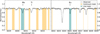 |
Fig. 3 Observed spectrum of the Z06-star in black with a SNR of 65. The line mask placements for the Mo (left) and Eu (right) line can be seen in turquoise and the continuum placements in yellow. |
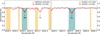 |
Fig. 4 As Fig. 3, the observed spectrum of the Z06-star can be seen in black. The line mask placements for the Mo (left) and Eu (right) line can be seen in turquoise and the continuum placements in yellow. The best fit to the synthetic spectrum is shown with a solid red line and the ±0.1 dex with a shaded red. Note that the wavelength region is zoomed in compared to Fig. 3 to better show the fit of the synthetic spectrum. |
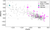 |
Fig. 5 [Mo/Fe] over [Fe/H] for the Z06-star (magenta star) and J13-star (teal diamond). We also show the bulge in [Mo/Fe] from Forsberg et al. (2022, magenta circles). The disc and halo with grey triangles are from (Peterson 2013; Hansen et al. 2014; Roederer et al. 2014; Mishenina et al. 2019; Forsberg et al. 2022). |
RA+Dec and proper motions from Gaia EDR3, (Gaia Collaboration 2016, 2021).
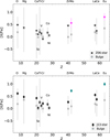 |
Fig. 6 [X/Fe] over Z for the bulge abundances (grey) presented in the Jönsson-series (Jönsson et al. 2017b; Lomaeva et al. 2019; Forsberg et al. 2019, 2022) for the Z06-star (upper plot, indicated with a star-symbol and the estimated uncertainties) and Johnson et al. (2013)-star (lower plot, indicated with a diamond). The bulge abundances are indicated by the mean (grey box) with the highest and lowest value (the Z06-star excluded) indicated by the bar, showing the spread in abundance in the bulge sample. To facilitate the reading of the plot, the element corresponding to a certain Z has been indicated. The r-process elements Mo and Eu has been indicated using magenta (Z06-star) and teal (J13-star). |
5.2 The orbits
In Fig. 7 we show the orbits for both stars. The J13-star makes clear deviations to both high |z| > 5 kpc and even passes outside of the Sun’s orbit in x–y plane. We also estimate the orbital parameters taking into account the derived uncertainties in distance and proper motion, and find that the distance is the parameter that makes the largest difference, and the proper motion is less important when the uncertainty in the distance is large. In Fig. 8, we show the orbits with the low and high distance estimates (as taken from Table 3) using the nominal proper motions. The Z06-star always remains in the bulge, given its smaller uncertainty in distance, whereas the J13-star is heavily affected by its distance. For the lower distance of the J13-star, it extends to |z| ~ 3 kpc, and seems to trace the bar potential adopted in the GalPy-setup (see Sect. 4.2).
As for the distances of the stars, we do note that both stars have distance estimates in Bailer-Jones et al. (2021), which uses a Bayesian approach and a prior model of the Galaxy. The distances are estimated to  pc and
  pc for the J13-star and the Z06-star, respectively3. We refer to Bailer-Jones et al. (2021) for more details on the distance measurements.
Similarly, the StarHorse code (SH, Queiroz et al. 2018), which also uses a Galactic prior, has distance estimates and stellar parameters to the stars using Gaia EDR3 and photometric catalogues in Anders et al. (2022). They give the distances to 6.1 kpc and 7.4 kpc, respectively, for the J13-star and the Z06-star.
These distance measurements puts the J13-star within the bulge, however, we also do note that the metallicity output from SH is very high, −0.38 dex, compared to −1.67 dex from the spectroscopic measurements (Johnson et al. 2013). Similarly, they estimated a 0.18 dex metallicity for the Z06-star, indicating large uncertainties when determining metallicities for very distant stars, which propagate to the estimated distances. Additionally, the parallax error in Gaia EDR3 for this star is as high as a quarter of the parallax (parallax_over_error of 3.9), implying that the parallax, used in Bailer-Jones et al. (2021), is unreliable. In conclusion, given the low metallicity and considering our distance- and orbital estimates of the J13-star, it seems likely that it has its origin in the Galactic halo or thick disc.
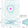 |
Fig. 7 Orbit for the J13-star (teal) and the Z06-star (magenta) plotted in x–y (top), x–z (bottom left) and R-z (bottom right) plane. The orbits are integrated over 10 Gyr and the position of the stars in their orbits are indicated, as well as the position of the Sun (yellow dot). This is the nominal case for the distances (“d”), which are indicated in the legend, and seen in Table 3. |
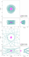 |
Fig. 8 Orbits for the J13-star (teal) and the Z06-star (magenta) plotted in x–y, x–z and R–z plane (as in Fig. 7). The position of the stars in their orbits are indicated, as well as the position of the Sun (yellow dot). The top figure show the orbits computed with the low distance estimate (“d”), and the bottom one with the high distance estimate, as indicated in the legend. Similarly as the nominal case, we integrate the orbits for 10 Gyr. |
6 Conclusions
In this work, we present an r-process enriched bulge star, 2MASS J18082459-2548444 (the Z06-star). We show that it is high in both molybdenum with [Mo/Fe] = 0.62 dex and europium with [Eu/Fe] = 0.78 dex, whilst having otherwise overall bulge-like abundances for other heavy trans-iron elements. Furthermore, the low [Ce,La/Eu] ratio suggests that the heavier trans-iron elements in the Z06-star were predominantly produced by the r-process, rather than the s-process.
We compared the star to the previously published r-enriched star in the bulge, MASS J18174532-3353235 (the J13-star), and estimated both stars’ distances and orbits. We find that the Z06-star likely is confined and has an origin in the bulge, whilst the J13-star is more probable to have a halo or thick disc origin. Nonetheless, we cannot firmly exclude that it resides in the bulge or that it has bulge origin, since distance measurements of stars at these distances in general come with large uncertainties.
It would be beneficial to measure the ruthenium (Ru, Z = 44) abundance of the Z06-star, which has a 7% p-process and 59% contribution from the r-process at solar metallicities. The J13-star is extremely high in Ru, [Ru/Fe] = 1.58 dex, which could suggests that intermediate mass elements such as Ru and Mo are produced in a distinct way (possibly the p-process in the case for Ru and Mo). However, all Ru-lines in the optical, such as the 5309 Å and 5699 Å line used in Johnson et al. (2013), lie outside of the spectrum range of 5800–6800 Å for the Z06-star, and new high-resolution spectra covering the whole optical region would be beneficial to be able to determine more trans-iron elements. The use of high-resolution, high S/N optical spectra is key in the search for these r-process enhanced stars; the r-process signatures are difficult to infer in the infrared (so far, only the r-process element ytterbium has had successful abundance determination in the infrared from high-resolution IGRINS spectra, as, for instance, in Montelius et al. 2022).
The discovery of one r-process enhanced star that is a member of the bulge does not independently provide insight into the bulge formation process. What this does is demonstrate, despite the significantly higher metallicities and implied greater rate of enrichment that it has been possible for sufficient r-process elements to be produced for a star such as the Z06-star could be discovered in the inner bulge. It is interesting to consider whether the tail of stars toward [Fe/H] ~ − 1 dex reflects an early period of enrichment in the history of the inner bulge and bar – and, as such, whether other signatures of stochastic production of elements in the early bulge might be found with subsequent studies.
We do have evidence to support that the inner halo at b = −11° (Koch et al. 2006) is interesting in this regard and that even small surveys find stars with unusual composition, including s- and p-process enhancements (Koch et al. 2016, 2019). However, it is important to emphasise that these stars, along with other recent surveys that emphasise the discovery of stars with [Fe/H] < −2 dex (e.g. EMBLA and Pristine Inner Galaxy Survey, Howes et al. 2016; Arentsen et al. 2020, respectively) explore a different potential discovery space, namely, that of the early inner halo. The importance of the Z06-star is rooted in strong evidence supporting its presence in the inner bulge and its [Fe/H] > −1 dex. The discovery of other stars similar to it, and residing in the tail toward −1 dex of the primary bulge metallicity distribution, might preserve the history of the enrichment event that gave rise to the chemical fingerprint associated with the formation of the bar. Alternatively, the low metallicity tail might preserve the record of an early merger. The discovery of additional similar stars and the detailed exploration of this population might provide new insights into the early formation history of the bulge.
Acknowledgements
We thank the anonymous referees for comments and suggestions that helped improve the manuscript. We thank Paul McMillan for discussions on Galactic potentials and distance estimates. R.F.’s research is supported by the Göran Gustafsson Foundation for Research in Natural Sciences and Medicine. R.F. and N.R. acknowledge support from the Royal Physiographic Society in Lund through the Stiftelse Walter Gyllenbergs fond and Märta och Erik Holmbergs donation. N.N. and M.S. acknowledge the funding of the BQR Lagrange. R.M.R. acknowledges the financial support and hospitality of the Observatoire de Côte d’Azur. B.T. acknowledges the financial support from the Japan Society for the Promotion of Science as a JSPS International Research Fellow. This work has made use of data from the European Southern Observatory (ESO) and the European Space Agency’s (ESA) Gaia mission (https://www.cosmos.esa.int/gaia), processed by the Gaia Data Processing and Analysis Consortium (DPAC, https://www.cosmos.esa.int/web/gaia/dpac/consortium). Funding for the DPAC has been provided by national institutions, in particular the institutions participating in the Gaia Multilateral Agreement. Software: NumPy (Harris et al. 2020), Matplotlib (Hunter 2007), GalPy (http://github.com/jobovy/galpy, Bovy 2015), AstroPy (Astropy Collaboration 2013).
References
- Anders, F., Khalatyan, A., Queiroz, A. B. A., et al. 2022, A&A, 658, A91 [NASA ADS] [CrossRef] [EDP Sciences] [Google Scholar]
- Arentsen, A., Starkenburg, E., Martin, N. F., et al. 2020, MNRAS, 496, 4964 [NASA ADS] [CrossRef] [Google Scholar]
- Astropy Collaboration (Robitaille, T. P., et al.) 2013, A&A, 558, A33 [NASA ADS] [CrossRef] [EDP Sciences] [Google Scholar]
- Bailer-Jones, C. A. L., Rybizki, J., Fouesneau, M., Demleitner, M., & Andrae, R. 2021, AJ, 161, 147 [Google Scholar]
- Bensby, T., Feltzing, S., Gould, A., et al. 2017, A&A, 605, A89 [NASA ADS] [CrossRef] [EDP Sciences] [Google Scholar]
- Bisterzo, S., Travaglio, C., Gallino, R., Wiescher, M., & Käppeler, F. 2014, ApJ, 787, 10 [NASA ADS] [CrossRef] [Google Scholar]
- Bovy, J. 2015, ApJS, 216, 29 [NASA ADS] [CrossRef] [Google Scholar]
- Bressan, A., Marigo, P., Girardi, L., et al. 2012, MNRAS, 427, 127 [NASA ADS] [CrossRef] [Google Scholar]
- Burbidge, E. M., Burbidge, G. R., Fowler, W. A., & Hoyle, F. 1957, Rev. Mod. Phys., 29, 547 [NASA ADS] [CrossRef] [Google Scholar]
- Cardelli, J. A., Clayton, G. C., & Mathis, J. S. 1989, ApJ, 345, 245 [Google Scholar]
- Cescutti, G., & Matteucci, F. 2022, Universe, 8, 173 [NASA ADS] [CrossRef] [Google Scholar]
- Cescutti, G., Romano, D., Matteucci, F., Chiappini, C., & Hirschi, R. 2015, A&A, 577, A139 [NASA ADS] [CrossRef] [EDP Sciences] [Google Scholar]
- Christlieb, N., Beers, T. C., Barklem, P. S., et al. 2004, A&A, 428, 1027 [NASA ADS] [CrossRef] [EDP Sciences] [Google Scholar]
- Clarkson, W., Sahu, K., Anderson, J., et al. 2008, ApJ, 684, 1110 [NASA ADS] [CrossRef] [Google Scholar]
- Côté, B., Eichler, M., Arcones, A., et al. 2019, ApJ, 875, 106 [Google Scholar]
- Cowan, J. J., Sneden, C., Burles, S., et al. 2002, ApJ, 572, 861 [NASA ADS] [CrossRef] [Google Scholar]
- Cutri, R. M., Skrutskie, M. F., van Dyk, S., et al. 2003, VizieR Online Data Catalog: II/246 [Google Scholar]
- Dehnen, W. 2000, AJ, 119, 800 [NASA ADS] [CrossRef] [Google Scholar]
- Di Matteo, P., Haywood, M., Gómez, A., et al. 2014, A&A, 567, A122 [NASA ADS] [CrossRef] [EDP Sciences] [Google Scholar]
- Forsberg, R., Jönsson, H., Ryde, N., & Matteucci, F. 2019, A&A, 631, A113 [NASA ADS] [CrossRef] [EDP Sciences] [Google Scholar]
- Forsberg, R., Ryde, N., Jönsson, H., Rich, R. M., & Johansen, A. 2022, A&A, 666, A125 [NASA ADS] [CrossRef] [EDP Sciences] [Google Scholar]
- Gaia Collaboration (Prusti, T., et al.) 2016, A&A, 595, A1 [NASA ADS] [CrossRef] [EDP Sciences] [Google Scholar]
- Gaia Collaboration (Brown, A. G. A., et al.) 2021, A&A, 649, A1 [NASA ADS] [CrossRef] [EDP Sciences] [Google Scholar]
- Gonzalez, O. A., Rejkuba, M., Zoccali, M., et al. 2011, A&A, 530, A54 [NASA ADS] [CrossRef] [EDP Sciences] [Google Scholar]
- Gonzalez, O. A., Rejkuba, M., Zoccali, M., et al. 2012, A&A, 543, A13 [NASA ADS] [CrossRef] [EDP Sciences] [Google Scholar]
- Grevesse, N., Scott, P., Asplund, M., & Sauval, A. J. 2015, A&A, 573, A27 [CrossRef] [EDP Sciences] [Google Scholar]
- Gustafsson, B., Edvardsson, B., Eriksson, K., et al. 2008, A&A, 486, 951 [NASA ADS] [CrossRef] [EDP Sciences] [Google Scholar]
- Hansen, C. J., Andersen, A. C., & Christlieb, N. 2014, A&A, 568, A47 [NASA ADS] [CrossRef] [EDP Sciences] [Google Scholar]
- Harris, C. R., Millman, K. J., van der Walt, S. J., et al. 2020, Nature, 585, 357 [NASA ADS] [CrossRef] [Google Scholar]
- Heiter, U., Jofré, P., Gustafsson, B., et al. 2015, A&A, 582, A49 [NASA ADS] [CrossRef] [EDP Sciences] [Google Scholar]
- Heiter, U., Lind, K., Bergemann, M., et al. 2021, A&A, 645, A106 [EDP Sciences] [Google Scholar]
- Hirai, Y., Ishimaru, Y., Saitoh, T. R., et al. 2015, ApJ, 814, 41 [NASA ADS] [CrossRef] [Google Scholar]
- Holmbeck, E. M., Hansen, T. T., Beers, T. C., et al. 2020, ApJS, 249, 30 [NASA ADS] [CrossRef] [Google Scholar]
- Howes, L. M., Asplund, M., Keller, S. C., et al. 2016, MNRAS, 460, 884 [NASA ADS] [CrossRef] [Google Scholar]
- Hunter, J. D. 2007, Comput. Sci. Eng., 9, 90 [NASA ADS] [CrossRef] [Google Scholar]
- Jeon, M., Besla, G., & Bromm, V. 2021, MNRAS, 506, 1850 [NASA ADS] [CrossRef] [Google Scholar]
- Jofré, P., Heiter, U., Soubiran, C., et al. 2014, A&A, 564, A133 [NASA ADS] [CrossRef] [EDP Sciences] [Google Scholar]
- Jofré, P., Heiter, U., Soubiran, C., et al. 2015, A&A, 582, A81 [Google Scholar]
- Johnson, C. I., Rich, R. M., Fulbright, J. P., Valenti, E., & McWilliam, A. 2011, ApJ, 732, 108 [NASA ADS] [CrossRef] [Google Scholar]
- Johnson, C. I., Rich, R. M., Kobayashi, C., & Fulbright, J. P. 2012, ApJ, 749, 175 [NASA ADS] [CrossRef] [Google Scholar]
- Johnson, C. I., McWilliam, A., & Rich, R. M. 2013, ApJ, 775, L27 [NASA ADS] [CrossRef] [Google Scholar]
- Johnson, C. I., Rich, R. M., Kobayashi, C., Kunder, A., & Koch, A. 2014, AJ, 148, 67 [Google Scholar]
- Johnson, C. I., Rich, R. M., Young, M. D., et al. 2020, MNRAS, 499, 2357 [NASA ADS] [CrossRef] [Google Scholar]
- Jönsson, H., Ryde, N., Nordlander, T., et al. 2017a, A&A, 598, A100 [NASA ADS] [CrossRef] [EDP Sciences] [Google Scholar]
- Jönsson, H., Ryde, N., Schultheis, M., & Zoccali, M. 2017b, A&A, 600, C2 [NASA ADS] [CrossRef] [EDP Sciences] [Google Scholar]
- Joyce, M., Johnson, C. I., Marchetti, T., et al. 2022, ApJ, submitted [arXiv:2205.07964] [Google Scholar]
- Karakas, A. I., & Lattanzio, J. C. 2014, PASA, 31, e030 [NASA ADS] [CrossRef] [Google Scholar]
- Kobayashi, C., Karakas, A. I., & Lugaro, M. 2020, ApJ, 900, 179 [Google Scholar]
- Koch, A., Grebel, E. K., Wyse, R. F. G., et al. 2006, AJ, 131, 895 [Google Scholar]
- Koch, A., McWilliam, A., Preston, G. W., & Thompson, I. B. 2016, A&A, 587, A124 [NASA ADS] [CrossRef] [EDP Sciences] [Google Scholar]
- Koch, A., Reichert, M., Hansen, C. J., et al. 2019, A&A, 622, A159 [NASA ADS] [CrossRef] [EDP Sciences] [Google Scholar]
- Kordopatis, G., Schultheis, M., McMillan, P. J., et al. 2022, A&A, in press, [arXiv.2206.07937] [Google Scholar]
- Launhardt, R., Zylka, R., & Mezger, P. G. 2002, A&A, 384, 112 [NASA ADS] [CrossRef] [EDP Sciences] [Google Scholar]
- Lecureur, A., Hill, V., Zoccali, M., et al. 2007, A&A, 465, 799 [NASA ADS] [CrossRef] [EDP Sciences] [Google Scholar]
- Lomaeva, M., Jönsson, H., Ryde, N., Schultheis, M., & Thorsbro, B. 2019, A&A, 625, A141 [NASA ADS] [CrossRef] [EDP Sciences] [Google Scholar]
- Majewski, S. R., Schiavon, R. P., Frinchaboy, P. M., et al. 2017, AJ, 154, 94 [NASA ADS] [CrossRef] [Google Scholar]
- Marigo, P., Girardi, L., Bressan, A., et al. 2017, ApJ, 835, 77 [Google Scholar]
- Matsuno, T., Hirai, Y., Tarumi, Y., et al. 2021, A&A, 650, A110 [NASA ADS] [CrossRef] [EDP Sciences] [Google Scholar]
- Matteucci, F., & Brocato, E. 1990, ApJ, 365, 539 [CrossRef] [Google Scholar]
- Matteucci, F., Romano, D., Arcones, A., Korobkin, O., & Rosswog, S. 2014, MNRAS, 438, 2177 [Google Scholar]
- McWilliam, A. 2016, PASA, 33, e040 [NASA ADS] [CrossRef] [Google Scholar]
- McWilliam, A., & Rich, R. M. 1994, ApJS, 91, 749 [NASA ADS] [CrossRef] [Google Scholar]
- McWilliam, A., Preston, G. W., Sneden, C., & Searle, L. 1995, AJ, 109, 2757 [Google Scholar]
- Mishenina, T. V., Pignatari, M., Korotin, S. A., et al. 2013, A&A, 552, A128 [NASA ADS] [CrossRef] [EDP Sciences] [Google Scholar]
- Mishenina, T., Pignatari, M., Gorbaneva, T., et al. 2019, MNRAS, 489, 1697 [NASA ADS] [CrossRef] [Google Scholar]
- Monari, G., Famaey, B., Siebert, A., et al. 2016, MNRAS, 461, 3835 [Google Scholar]
- Montelius, M., Forsberg, R., Ryde, N., et al. 2022, A&A, 665, A135 [NASA ADS] [CrossRef] [EDP Sciences] [Google Scholar]
- Ness, M., Freeman, K., Athanassoula, E., et al. 2012, ApJ, 756, 22 [NASA ADS] [CrossRef] [Google Scholar]
- Ness, M., Freeman, K., Athanassoula, E., et al. 2013, MNRAS, 430, 836 [NASA ADS] [CrossRef] [Google Scholar]
- Nishimura, S., Kotake, K., Hashimoto, M.-A., et al. 2006, ApJ, 642, 410 [Google Scholar]
- Ortolani, S., Renzini, A., Gilmozzi, R., et al. 1995, Nature, 377, 701 [CrossRef] [Google Scholar]
- Peterson, R. C. 2013, ApJ, 768, L13 [NASA ADS] [CrossRef] [Google Scholar]
- Piskunov, N., & Valenti, J. A., 2017, A&A, 597, A16 [NASA ADS] [CrossRef] [EDP Sciences] [Google Scholar]
- Prantzos, N., Abia, C., Cristallo, S., Limongi, M., & Chieffi, A. 2020, MNRAS, 491, 1832 [Google Scholar]
- Queiroz, A. B. A., Anders, F., Santiago, B. X., et al. 2018, MNRAS, 476, 2556 [Google Scholar]
- Rauscher, T., Dauphas, N., Dillmann, I., et al. 2013, Rep. Progr. Phys., 76, 066201 [CrossRef] [Google Scholar]
- Renzini, A., Gennaro, M., Zoccali, M., et al. 2018, ApJ, 863, 16 [NASA ADS] [CrossRef] [Google Scholar]
- Rich, R. M. 1988, AJ, 95, 828 [NASA ADS] [CrossRef] [Google Scholar]
- Roederer, I. U., Preston, G. W., Thompson, I. B., et al. 2014, AJ, 147, 136 [Google Scholar]
- Roederer, I. U., Lawler, J. E., Den Hartog, E. A., et al. 2022, ApJS, 260, 27 [NASA ADS] [CrossRef] [Google Scholar]
- Rojas-Arriagada, A., Recio-Blanco, A., de Laverny, P., et al. 2017, A&A, 601, A140 [NASA ADS] [CrossRef] [EDP Sciences] [Google Scholar]
- Rojas-Arriagada, A., Zasowski, G., Schultheis, M., et al. 2020, MNRAS, 499, 1037 [Google Scholar]
- Ryde, N., Gustafsson, B., Edvardsson, B., et al. 2010, A&A, 509, A20 [CrossRef] [EDP Sciences] [Google Scholar]
- Scott, P., Asplund, M., Grevesse, N., Bergemann, M., & Sauval, A. J. 2015a, A&A, 573, A26 [NASA ADS] [CrossRef] [EDP Sciences] [Google Scholar]
- Scott, P., Grevesse, N., Asplund, M., et al. 2015b, A&A, 573, A25 [NASA ADS] [CrossRef] [EDP Sciences] [Google Scholar]
- Shen, J., Rich, R. M., Kormendy, J., et al. 2010, ApJ, 720, L72 [NASA ADS] [CrossRef] [Google Scholar]
- Sneden, C., Cowan, J. J., Lawler, J. E., et al. 2003, ApJ, 591, 936 [NASA ADS] [CrossRef] [Google Scholar]
- Sneden, C., Cowan, J. J., & Gallino, R. 2008, ARA&A, 46, 241 [Google Scholar]
- Valenti, J. A. & Piskunov, N. 1996, A&AS, 118, 595 [NASA ADS] [CrossRef] [EDP Sciences] [Google Scholar]
- Van der Swaelmen, M., Barbuy, B., Hill, V., et al. 2016, A&A, 586, A1 [NASA ADS] [CrossRef] [EDP Sciences] [Google Scholar]
- Vasiliev, E. 2019, MNRAS, 482, 1525 [Google Scholar]
- Weiland, J. L., Arendt, R. G., Berriman, G. B., et al. 1994, ApJ, 425, L81 [NASA ADS] [CrossRef] [Google Scholar]
- Zasowski, G., Schultheis, M., Hasselquist, S., et al. 2019, ApJ, 870, 138 [NASA ADS] [CrossRef] [Google Scholar]
- Zoccali, M., Lecureur, A., Barbuy, B., et al. 2006, A&A, 457, L1 [NASA ADS] [CrossRef] [EDP Sciences] [Google Scholar]
- Zoccali, M., Hill, V., Lecureur, A., et al. 2008, A&A, 486, 177 [NASA ADS] [CrossRef] [EDP Sciences] [Google Scholar]
Available at https://marcs.astro.uu.se.
La and Ce has a roughly 75% and 85% origin from the s-process at solar metallicities, respectively (Bisterzo et al. 2014; Prantzos et al. 2020).
Note: this is the geometric distance as measured by Bailer-Jones et al. (2021), the photogeometric, which combines the geometric with G-magnitude and BP-RP colours, gives  pc and
  pc respectively, for J13-star and Z06-star. In general, the photogeometric distance extend to larger distances and tend to have smaller uncertainties.
All Tables
Comparison of the stellar parameters (Cols. 2-5) for the Z06-star from five different spectroscopic studies (Col. 1).
Determined absolute abundances A(X) and solar- and metallicity-normalised abundances [X/Fe] of the Z06-star.
All Figures
|
Fig. 1 Map of the Galactic bulge, showing the position of the Z06-star, 2MASS J18082459-2548444 (magenta), and the J13-star, 2MASS J18174532-3353235 (teal), presented in this work. The dust extinction towards the bulge is taken from Gonzalez et al. (2011, 2012) and scaled to optical extinction (Cardelli et al. 1989). The scale saturates at AV = 2, setting the upper limit. We also plot the COBE/DIRBE outlines of the Galactic bulge (Weiland et al. 1994). |
| In the text | |
|
Fig. 2 [Eu/Fe] over [Fe/H] for the Z06-star (magenta star) and the J13-star (teal diamond). For reference, we plot the bulge (magenta circles) and disc stars (grey squares) from Forsberg et al. (2019) as well as the bulge stars from Johnson et al. (2012). The abundances of the halo stars come from the r-process alliance sample (dark grey triangles Holmbeck et al. 2020). The orange line indicates the ‘r-II’ limit as defined in the r-process alliance (Holmbeck et al. 2020). We note that the abundances from Forsberg et al. (2019) have been systematically lowered with 0.10 dex, as described in Sect. 3.1. |
| In the text | |
|
Fig. 3 Observed spectrum of the Z06-star in black with a SNR of 65. The line mask placements for the Mo (left) and Eu (right) line can be seen in turquoise and the continuum placements in yellow. |
| In the text | |
|
Fig. 4 As Fig. 3, the observed spectrum of the Z06-star can be seen in black. The line mask placements for the Mo (left) and Eu (right) line can be seen in turquoise and the continuum placements in yellow. The best fit to the synthetic spectrum is shown with a solid red line and the ±0.1 dex with a shaded red. Note that the wavelength region is zoomed in compared to Fig. 3 to better show the fit of the synthetic spectrum. |
| In the text | |
|
Fig. 5 [Mo/Fe] over [Fe/H] for the Z06-star (magenta star) and J13-star (teal diamond). We also show the bulge in [Mo/Fe] from Forsberg et al. (2022, magenta circles). The disc and halo with grey triangles are from (Peterson 2013; Hansen et al. 2014; Roederer et al. 2014; Mishenina et al. 2019; Forsberg et al. 2022). |
| In the text | |
|
Fig. 6 [X/Fe] over Z for the bulge abundances (grey) presented in the Jönsson-series (Jönsson et al. 2017b; Lomaeva et al. 2019; Forsberg et al. 2019, 2022) for the Z06-star (upper plot, indicated with a star-symbol and the estimated uncertainties) and Johnson et al. (2013)-star (lower plot, indicated with a diamond). The bulge abundances are indicated by the mean (grey box) with the highest and lowest value (the Z06-star excluded) indicated by the bar, showing the spread in abundance in the bulge sample. To facilitate the reading of the plot, the element corresponding to a certain Z has been indicated. The r-process elements Mo and Eu has been indicated using magenta (Z06-star) and teal (J13-star). |
| In the text | |
|
Fig. 7 Orbit for the J13-star (teal) and the Z06-star (magenta) plotted in x–y (top), x–z (bottom left) and R-z (bottom right) plane. The orbits are integrated over 10 Gyr and the position of the stars in their orbits are indicated, as well as the position of the Sun (yellow dot). This is the nominal case for the distances (“d”), which are indicated in the legend, and seen in Table 3. |
| In the text | |
|
Fig. 8 Orbits for the J13-star (teal) and the Z06-star (magenta) plotted in x–y, x–z and R–z plane (as in Fig. 7). The position of the stars in their orbits are indicated, as well as the position of the Sun (yellow dot). The top figure show the orbits computed with the low distance estimate (“d”), and the bottom one with the high distance estimate, as indicated in the legend. Similarly as the nominal case, we integrate the orbits for 10 Gyr. |
| In the text | |
Current usage metrics show cumulative count of Article Views (full-text article views including HTML views, PDF and ePub downloads, according to the available data) and Abstracts Views on Vision4Press platform.
Data correspond to usage on the plateform after 2015. The current usage metrics is available 48-96 hours after online publication and is updated daily on week days.
Initial download of the metrics may take a while.