| Issue |
A&A
Volume 666, October 2022
|
|
|---|---|---|
| Article Number | A125 | |
| Number of page(s) | 12 | |
| Section | Stellar atmospheres | |
| DOI | https://doi.org/10.1051/0004-6361/202244013 | |
| Published online | 18 October 2022 | |
Abundances of disk and bulge giants from high-resolution optical spectra
V. Molybdenum: The p-process element★,★★
1
Lund Observatory, Department of Astronomy and Theoretical Physics, Lund University,
Box 43,
22100
Lund, Sweden
e-mail: rebecca@astro.lu.se
2
Materials Science and Applied Mathematics, Malmö University,
205 06
Malmö, Sweden
3
Department of Physics and Astronomy, ICLA,
430 Portola Plaza,
Box 951547,
Los Angeles, CA
90095-1547, USA
4
Center for Star and Planet Formation, GLOBE Institute University of Copenhagen,
Øster Voldgade 5-7,
1350
Copenhagen, Denmark
Received:
10
May
2022
Accepted:
27
June
2022
Aims. In this work, we aim to make a differential comparison of the neutron-capture and p-process element molybdenum (Mo) in the stellar populations in the local disk(s) and the bulge, focusing on minimising possible systematic effects in the analysis.
Methods. The stellar sample consists of 45 bulge and 291 local disk K-giants observed with high-resolution optical spectra. The abundances are determined by fitting synthetic spectra using the Spectroscopy Made Easy (SME) code. The disk sample is separated into thin and thick disk components using a combination of abundances and kinematics. The cosmic origin of Mo is investigated and discussed by comparing with published abundances of Mo and the neutron-capture elements cerium (Ce) and europium (Eu).
Results. We determine reliable Mo abundances for 35 bulge and 282 disk giants with a typical uncertainty of [Mo/Fe] ~ 0.2 and ~0.1 dex for the bulge and disk, respectively.
Conclusions. We find that the bulge is possibly enhanced in [Mo/Fe] compared to the thick disk, which we do not observe in either [Ce/Fe] or [Eu/Fe]. This might suggest a higher past star-formation rate in the bulge; however, as we do not observe the bulge to be enhanced in [Eu/Fe], the origin of the molybdenum enhancement is yet to be constrained. Although the scatter is large, we may be observing evidence of the p-process contributing to the heavy element production in the chemical evolution of the bulge.
Key words: stars: abundances / Galaxy: abundances / Galaxy: bulge / Galaxy: disk / Galaxy: evolution / solar neighborhood
Full Tables A.1–A.4 are only available at the CDS via anonymous ftp to cdsarc.u-strasbg.fr (130.79.128.5) or via http://cdsarc.u-strasbg.fr/viz-bin/cat/J/A+A/666/A125
Based on observations made with the Nordic Optical Telescope (programs 51-018 and 53-002) operated by the Nordic Optical Telescope Scientific Association at the Observatorio del Roque de los Muchachos, La Palma, Spain, of the Instituto de Astrofisica de Canarias, spectral data retrieved from PolarBase at Observatoire Midi Pyrénées, and observations collected at the European Southern Observatory, Chile (ESO programs 71.B-0617(A), 073.B-0074(A), and 085.B-0552(A)).
© R. Forsberg et al. 2022
 Open Access article, published by EDP Sciences, under the terms of the Creative Commons Attribution License (https://creativecommons.org/licenses/by/4.0), which permits unrestricted use, distribution, and reproduction in any medium, provided the original work is properly cited.
This article is published in open access under the Subscribe-to-Open model. Subscribe to A&A to support open access publication.
1 Introduction
Elemental abundances of stars have proven to be key both in tracing the chemical evolution of the Milky Way and to our understanding of the origin of the elements themselves. Stars carry a chemical fingerprint from the molecular cloud from which they formed, which can be measured in their photospheres. The Galaxy is enriched with elements over time, where they are formed in various processes, either internally in stars or in more explosive environments such as type Ia and II supernovae (SNe) and neutron star mergers (NSM).
By measuring the chemical abundances in stars of a range of metallicities, [Fe/H], we can trace the evolution of elements and, in turn, the stellar populations that make up the Milky Way. In this work, we focus on the disk components (thin and thick) and the bulge. The origin and evolution of the bulge have attracted much attention, and the bulge has been re-defined from a classical, spherical bulge to now being primarily classified as a pseudo-bulge with a box/peanut bar (e.g. Ness et al. 2012; Di Matteo et al. 2014; Shen & Zheng 2020). The connection of the bulge or bar to the disk structure remains central, and careful, detailed abundance studies reveal surprisingly small differences between the composition of the bulge and the thick disk (Jönsson et al. 2017b; Lomaeva et al. 2019; Forsberg et al. 2019). While it is agreed that the bulge metallicities reach values higher than those of the thick disk (Matteucci & Brocato 1990; McWilliam 2016), there remains no convincing difference in abundance trends (see e.g. Barbuy et al. 2018, and references therein). A careful differential comparison between the bulge and the disk is needed, and while many such studies are published, ours employs newly reduced and analysed high-quality data sets.
In this series of articles, (Jönsson et al. 2017a,b; Lomaeva et al. 2019; Forsberg et al. 2019, hereafter referred to as Paper I, Paper II, Paper III, Paper IV), the bulge chemistry is investigated by a differential comparison to a disk sample. The two stellar populations have been analysed with the same method, atomic data, and set of spectral lines from high-resolution spectra of 291 disk giants and 45 bulge giants in order to minimise the systematic uncertainties in the analysis. In particular, using the same type of star removes the possible systematic difference in abundance between dwarf and giant stars (see e.g. Meléndez et al. 2008; Gonzalez & Gadotti 2016). In the previous papers of this series we present findings supporting that the bulge has a similar evolutionary history to the thick disk, although we cannot exclude possible relative enrichment in some elements, such as vanadium (V), cobalt (Co) (Paper III), and lanthanum (La) (Paper IV) in the bulge.
In Paper IV, we investigated the neutron-capture elements Zr, La, Ce, and Eu. These are produced through neutron-capture processes (Cameron 1957; Burbidge et al. 1957), which is the process responsible for creating more than two-thirds of the periodic table of elements. These can add an additional piece to the puzzle in Galactic archaeology, because these neutron-capture elements are different from both the α- and iron-peak elements which have primarily SNe type II and SNe type Ia origin.
The neutron-capture process involves two physical processes. The capture of a neutron onto a seed atom, creating a heavier isotope, and the possible subsequent β− – decay, n → p + e− + ve, creating a heavier element. As a consequence, the neutron-capture and β− –decay outline two sub-processes, the slow s-process, and the rapid r-process.
While it is usual to refer to elements as primarily being either s- or r-process elements, in virtually all cases, both r- and s-processes contribute. An r-process element is an element with a dominant origin from the r-process in the Sun, and vice versa for s-process elements. However, it can be more informative to examine the origin of the (stable) isotopes that make up the element. For instance, europium (Eu, Z = 63) has two stable isotopes that each contribute roughly 50% to the solar Eu, 151Eu, and 153Eu (Bisterzo et al. 2014; Prantzos et al. 2020), where both of them have a dominating origin from the r-process, making Eu an r-process element. There are 35 stable isotopes that cannot be reached through either the s- or r-process and are instead formed in the so-called p-process (Cameron 1957; Burbidge et al. 1957); we discuss these in Sect. 5.
The element molybdenum1 (Mo, Z = 42) has seven stable isotopes, namely 92,94,95,96,97,98,100Mo and is an intriguing element because some of these isotopes are purely from the s-, r-, or p-processes. Both of the lightest ones, 92Mo and 94Mo, are p-isotopes, whereas 96Mo is a pure s-isotope and 100Mo is a pure r-isotope. Combined, the p-isotopes contribute roughly 20–25% of the solar Mo abundance, which is the highest contribution from the p-process seen in any element (as measured in the Sun, Prantzos et al. 2020). The second-highest contributing p-element is ruthenium (Ru, Z = 44) with roughly 7% of the solar ruthenium abundance (Prantzos et al. 2020). As such, Mo and its isotopes provide excellent benchmark examples for nuclear physics and astrophysics. Studying Mo from the perspective of Galactic chemical evolution can help to put constraints on the origin of this element, the origin of the p-process, and to constrain the evolution of the Galaxy itself.
The remaining contributions from the s- and r-process to Mo have varying values, where Bisterzo et al. (2014) report 39% of Mo production coming from the s-process, whereas Prantzos et al. (2020) instead give a 50% s-process and 27% r-process origin to Mo, at solar metallicities. However, it should be noted that the solar composition of molybdenum might not be representative of the Galactic composition often presented in Galactochemical evolution models. Measurements of meteorites show that the inner Solar System, especially the Earth, is relatively enriched in the s-process by high 96Mo values compared to 92,94Mo (p-process) and 95Mo (r-process dominated; Burkhardt et al. 2011; Budde et al. 2016, 2019). This means that the Mo isotopic composition of Earth can be used to put constraints on the types of meteoric material that contributed to the formation of our planet. The meteoric isotopic composition has been suggested to be affected by the origin of the dust that makes up the meteorites (Lugaro et al. 2016; Ek et al. 2020). This makes Mo a particularly interesting target for study and means that putting further constraints on its cosmic origin could be of significant value.
Larger published samples of Mo abundances for stars in the disk and bulge are sparse. Mishenina et al. (2019) determined Mo abundances for roughly 200 dwarf disk stars, which complements previous abundances at metallicities of [Fe/H] < −1.2 dex (Peterson 2013; Roederer et al. 2014a; Hansen et al. 2014; Spite et al. 2018). However, in Galactic chemical evolution models, Mo has been consequently underestimated compared to observations (Mishenina et al. 2019). On the other hand, the models in Kobayashi et al. (2020), where v-winds are included (which is a suggested production channel for p-isotopes), overproduce Mo, indicating that constraining this element is problematic without proper knowledge and modelling of the p-process. By presenting abundances for Mo in both giants in the local disk and in the bulge, we aim to put further constraints on both the Galactochemical evolution of the bulge and the origin of Mo.
This paper is structured as follows: in Sect. 2 we present the spectroscopic data used. In Sect. 3, we present the methodology for the analysis of the data, which follows closely that of previous papers in this series. In Sect. 4, we present the abundances, the estimated uncertainties and a comparison with previous studies. Finally, in Sects. 5 and 6 we discuss our results and outline our conclusions.
2 Data
In this section, we introduce the data used in this work, where we aim to have high-resolution and high-signal-to-noise (S/N) spectra for our bulge- and disk giants.
2.1 Bulge
Optical high-resolution spectra of bulge giants are fairly rare, because of the long integration times needed for observing these stars. Additionally, observing bulge giants in the optical wavelength regime is a challenge in itself, given the high amount of dust causing extinction. The spectra used here were therefore collected from low-extinction regions in the bulge, or its vicinity, which can be seen in Fig. 1.
The spectra for stars in the B3, BW, B6, and BL fields (using the naming convention in Lecureur et al. 2007) were obtained in 2003–2004 whilst the SW field was obtained in 2011 (ESO program 085.B-0552(A)). All spectra were obtained with the UVES/FLAMES spectrograph (R ~ 47 000) mounted on the VLT and are limited to the wavelength regime of 5800–6800 Å. The S/N (see Paper I, for details of the S/N estimation) are generally around 50; see Table A.3 for details of all the bulge giants and their spectra.
The spectra from the B3, BW, B6, and BL fields were first used in Zoccali et al. (2006) and were reanalysed in several subsequent articles, such as Lecureur et al. (2007); Van der Swaelmen et al. (2016). In Papers II; III; IV, we reanalyse 27 of these bulge stars, plus the additional 18 stars in the low-extinction SW field, which brings the total number of bulge stars analysed in this paper to 45. The reader is referred to Paper II for further details of the bulge sample.
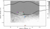 |
Fig. 1 Map of the Galactic bulge showing the five analysed fields, B3, BW, B6, BL (using the naming convention in Lecureur et al. 2007), and SW. The dust extinction towards the bulge is taken from Gonzalez et al. (2011, 2012) and scaled to optical extinction (Cardelli et al. 1989). The scale saturates at AV = 2, which is the upper limit in the figure. The COBE/DIRBE contours of the Galactic bulge, in black, are from Weiland et al. (1994). |
2.2 Disk
The disk sample consists of 291 giant local disk stars, 272 of which were observed by us using the FIbre-fed Echelle Spectrograph (FIES; Telting et al. 2014) mounted on the Nordic Optical Telescope, Roque de Los Muchachos, La Palma, and 19 spectra are downloaded from the PolarBase data base (Petit et al. 2014), in turn coming from the ESPaDOnS and NARVAL spectrographs (mounted on Canada–France–Hawaii Telescope and Telescope Bernard Lyot, respectively). The FIES and Polar-Base spectrographs have similar resolutions of R ~ 67 000 and R ~ 65 000, respectively, and wavelength coverage of 3700–8300 Å and 3700–10 500 Å, respectively. However, we note that we only use the 5800–6800 Å wavelength regime, to match that of the bulge spectra and to only use the same spectral lines in the analysis. The FIES spectra have a S/N of around 80–120, whereas that of the PolarBase is lower, at around 30–50. All spectra are reduced using the standard automatic pipelines. See Table A.1 for details of all the disk giants and their spectra.
We plotted a telluric spectrum over the observed stellar spectra, namely the one in the Arcturus atlas (Hinkle et al. 1995), such that regions affected by telluric lines could be avoided on a star-by-star basis. Further details of the FIES observational programs and the disk spectra are found in Paper I.
3 Methodology
The methodology of the analysis in this work closely follows the methodology set out in the previous papers in this series: Paper I; Paper II; Paper III; Paper IV. In those previous papers, we obtain very tight abundance trends with metallicity, and we can see that a carefully chosen set of spectral lines is key to achieving these high-quality abundances. In this section, we go through the basic details of the analysis of the giant stars, especially focusing on the 6030 Å Mo I line.
3.1 Spectral analysis
The spectral analysis to obtain the stellar parameters and elemental abundances was carried out using the tool Spectroscopy Made Easy (Valenti & Piskunov 1996; Piskunov & Valenti 2017, SME, version 554). SME produces a synthetic spectrum using a χ2-minimisation to fit the observed spectrum. To produce a synthetic spectrum, SME requires:
A line list containing atomic- and/or molecular data. We use the Gaia-ESO line list version 6 as published in Heiter et al. (2021).
Model atmospheres; in this work use the grid of MARCS models2 (Gustafsson et al. 2008). As our stellar sample consists of giant stars, we use the MARCS models with spherical symmetry for log(g) < 3.5.
Stellar parameters; the ones used in this work were derived by Papers I; II, where more details can be found. Briefly, we use a combination of iron (Fe) and calcium (Ca) lines, namely Fe I and Fe II, Ca I, and log g sensitive Ca I line wings. The Fe I lines suffers from deviations from Local Thermodynamic Equilibrium (LTE) and we adopt non-LTE (NLTE) corrections from Lind et al. (2012). In Papers I; II, we also estimate typical uncertainties and compare with Gaia benchmark stars (Heiter et al. 2015; Jofré et al. 2014, 2015). In general, the stellar parameters compare well with the benchmark parameters. However, the surface gravities are likely systematically high from the benchmark comparison with +0.10 dex. Furthermore, comparing with StarHorse (Queiroz et al. 2018) surface gravities derived from Gaia EDR3 (Gaia Collaboration 2016, 2021; Anders et al. 2022), the Paper I surface gravities are also systematically +0.10 dex too high. This could cause some overestimation of the abundances, but the main scope of this work is to make a differential comparison between the disk and bulge sample, which will be equally systematically affected.
A defined spectral segment, within which the line of interest and local continuum is marked with a line mask, or continuum masks, respectively. By the manual placement of local continuum masks, the continuum is renormalised3 more carefully to the local segment around the spectral line of interest. SME uses the continuum masks to fit a straight line in between, creating the local continua.
The line mask around the line of interest, the Mo 16030 Åline in this case, is also defined manually. This manual placement of both line- and continuum masks has been shown to be crucial in order to get high-precision abundances (Paper I; Paper II; Paper III; Paper IV). The line mask and continuum masks can be seen in Fig. 2. We go into more details of the abundance determination below.
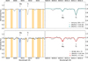 |
Fig. 2 Observed spectrum (black) for a disk star (top, Arcturus) and bulge star (bottom, B3–B8). Left: line mask placements for the Mo line marked in blue and the continuum placements in yellow. Right: synthetic spectra, either in teal (top, disk star Arcturus) or red (bottom, bulge star B3–B8). The estimated S/N of both spectra, 117 and 72 respectively, are indicated in the legend. We note that the wavelength region of the rightmost figures is zoomed in with respect to the leftmost figures. |
3.2 Abundance determination of Mo
In the abundance determination, we use the Mo I spectral line located at 6030 Å. The atomic data we use for this line come from the Gaia-ESO line list version 6 (Heiter et al. 2021); see Table 1. The spectral line is classified as a Yes/Yes line in the Gaia-ESO list, meaning that it has a high-quality log(gf)-value and is unblended. Furthermore, Heiter et al. (2021) report that this line should be avoided in abundance analyses of dwarf stars. As such, this line is a great example of a line that can only be reached in giant stars, where the lower surface gravities increase the line strength sufficiently for reliable abundances to be estimated.
Molybdenum does not have any hyperfine splitting (HFS) but has, as mentioned above, seven stable isotopes in the Sun. However, these are not included in the line list because the isotopic shift (IS) cannot be resolved, partly because of the Mo I lines being very weak. This means that we cannot measure the individual isotopic abundances, but rather the molybdenum abundance as a whole.
The observed and synthetic spectra close to the 6030 Å line can be seen in Fig. 2 for both a typical bright red giant disk star (Arcturus/α-Boo/HIP69673, in the top row) and one of the bulge stars (B3–B8, in the bottom row). Here, we also plot the line-and continuum segments used to produce the synthetic spectra. The same masks are used for all stars in the analysis for optimal coherence.
All synthetic spectra are examined by eye and the masks edited to return the best possible fit of the synthetic spectra to the observed spectrum. We were able to determine reliable synthetic spectra and, in turn, abundances for all stars where a line is detectable and above the noise. In instances where the spectral line is weaker than the noise, the line cannot be used to determine a reliable abundance. Nonetheless, using giant stars we are able to determine abundances for stars with a low molybdenum abundance because the line strengths typically increase with decreasing surface gravity. It should be noted that we determined all Mo abundances under the assumption of LTE. The 6030 Å line is a rather weak line, and forms in the deeper parts of the stellar atmosphere where collisions dominate, establishing LTE. As such, NLTE corrections for Mo should be small or negligible, which has been noted previously with smaller samples of stars (see e.g. Peterson 2011; Roederer et al. 2014b, 2022).
Atomic data for the Mo I atomic line.
3.3 Population separation
The separation of the disk components has been done using chemical and kinematical properties. As described in more detail in Paper III, we use [Ti/Fe] and [Fe/H] (determined in Paper I) as a proxy for the chemical separation typically observed in α-abundances. Additionally, we use Galactic space velocities as calculated with galpy (Bovy 2015) using radial velocities (see Table A.1), distances (McMillan 2018), and proper motions (Gaia Collaboration 2016, 2018) as input and calculate the total velocities,  . As Gaia has a limit on brightness, some of our brightest stars are not observed with Gaia, and kinematic data were available for a total of 268 of the disk stars. We then use the clustering method called Gaussian Mixture Model (GMM) – found in the scikit-learn module in Python (Pedregosa et al. 2011) – to cluster the disk data into the two components. As we use a combination of chemistry and kinematics, we refer to the components as thin and thick disk, where the thick disk is typically more α-rich and kinematically hotter than the thin disk.
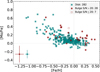 |
Fig. 3 [Mo/Fe] vs [Fe/H] for the disk (teal) and the bulge (red) in this study. The typical uncertainties, as described in Sect. 4.3 are indicated in the lower right corner. The grey dashed lines that go through [0, 0] indicate the solar value, which we have normalised to A (Fe) = 7.45 (Grevesse et al. 2007) and A(Mo) = 1.88 (Grevesse et al. 2015). |
4 Results
In this section, we introduce the abundances that we determined in this study, show a comparative plot with abundances from previous studies, as well as introduce the uncertainty estimates for the abundances from this study.
4.1 Abundances from this study
After manual inspection of the synthetic spectra, we end up with 282 stars in the local disk and 35 in the bulge with reliably determined Mo abundances. The detailed abundances for the disk and bulge giants can be found in Tables A.2 and A.4, respectively. The abundance ratio [Mo/Fe] plotted against the metallicity [Fe/H] for the stellar samples can be seen in Fig. 3. For consistency with the previous papers in this series, we make a distinction between bulge spectra with S/Ns of above and below 20. Nonetheless, as can be seen in Fig. 3, the bulge stars with S/N ≤ 20 are within the scatter of the overall bulge trend. The typical uncertainties are noted in the lower left corner of the plot. Our method of estimation of the uncertainties is described further in Sect. 4.3.
4.2 Abundances from previous studies
The separation of the disk components can be seen in Fig. 4, where we also compare with a disk sample from Mishenina et al. (2019). They published the first extended sample of Mo-abundances for stars in the Milky Way disk, which, together with halo observations (as described below), help to extend our knowledge of molybdenum. With our additional sample, we now extend the study of Mo even further, and provide a comparison giant sample to the disk abundances. The Mishenina et al. (2019) sample consists of 183 disk stars, where they identify 163 as thin and 20 as thick disk dwarf stars (determined using kinematics, Mishenina et al. 2013, 2019), whereas we identify 191 and 68 thin and thick disk giant stars. As such, we more than double and triple the thin and thick disk sample of Mo-abundances, respectively.
Mishenina et al. (2019) also have high-resolution spectra of R > 42 000 and S/N > 100. In the abundance analysis of Mo I of their dwarf sample, they use the spectral lines at 5506 and 5533 Å. These two lines have relatively strong blends, which can make abundance determination difficult (Heiter et al. 2021). As these two lines are outside of the spectral range for our bulge stars, we have not included these in our analysis. Additionally, the 6030 Å line that is used in our study is not accessible in dwarf stars, where it is very weak (see Sect. 3.2).
In Fig. 5, we plot some additional previous work in the more metal-poor regime of [Fe/H] < −1.2, which consists mainly of halo stars. Roederer et al. (2014a) uses the 3864 Å Mo I line to determine the Mo-abundances in both horizontal branch, main sequence, red giant, and subgiant stars. Altogether, they determine Mo in 279 low-metallicity stars (we note that the two metal-poor stars in Roederer et al. 2014b, are not included in Fig. 5). It is worth noting that even though the 3864 Å is not reachable in our sample, which is limited to 5800–6800 Å, the bluer wavelength regime would be very crowded with lines in giant stars at the metallicities of our stellar sample, making continuum placement extremely difficult.
In the work from Hansen et al. (2014) and Peterson (2013), the authors primarily also use the 3864 Å Mo I line to determine Mo abundances. While Peterson (2013) focuses on turnoff stars, Hansen et al. (2014) sample consists of dwarfs and giant stars, a total of 52. These latter authors have high-quality data with spectral resolution of R ~ 40 000 and S/N > 100. We note that in Fig. 5, we only plot the 40 stars that have abundances marked as high quality, which are not affected by large uncertainties due to blends and continuum placement (see Table 4 in Hansen et al. 2014). Finally, we also plot the Mo abundances of the 11 stars in Spite et al. (2018), who also use the bluer 3864 Å line. It should be noted that the star identified at [Fe/H] −3.06 with [Mo/Fe] of −0.38 is a r-poor star, BD–18 5550, explaining the low abundance.
There are also published Mo abundances for barium stars (Ba-stars). These are stars enriched in s-process elements, as well as in carbon, but otherwise have nominal abundances. These stars have been enriched due to accretion of s-process elements from a companion AGB-star, resulting in these peculiar abundances (Allen & Barbuy 2006; Roriz et al. 2021). As such, we do not include Ba-stars in the comparison plot with previous Mo abundances. Furthermore, Mo has been measured in the globular clusters M22 (Roederer et al. 2011) and 47 Tucanae (Thygesen et al. 2014), in open clusters (see e.g. Overbeek et al. 2016; Mishenina et al. 2020, among others), and in the r-process enhanced bulge star 2MASS J18174532–3353235 in Johnson et al. (2013). We note that these are not included in Fig. 5, where we look at the overall disk (and halo) trend in molybdenum.
Lastly, in Figs. 6 and 7, we compare the Mo abundance with the abundances of Ce (s-process) and Eu (r-process) from Paper IV. We discuss these figures further in Sect. 5 below.
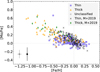 |
Fig. 4 Comparison of the [Mo/Fe] thin (blue squares) and thick (orange triangles) disk abundances determined in this work with the thin (black crosses) and thick (green diamonds) disk in Mishenina et al. (2019). It should be noted that the 23 stars that we do not have kinematical data for have not been classified as either thin or thick disk, and can be seen as grey circles. The typical uncertainties are indicated in the lower left corner (this work in grey, Mishenina et al. 2019 in black). The grey dashed lines that go through [0, 0] indicate the solar value, which we have normalised to A(Fe) = 7.45 (Grevesse et al. 2007) and A(Mo) = 1.88 (Grevesse et al. 2015). The thin disk star at [Fe/H] = −0.55 with high molybdenum abundance of [Mo/Fe] = 0.68, HIP65028, is discussed at the end of Sect. 5. |
4.3 Uncertainties
The random uncertainties that arise because of line- and continuum placements are hard to estimate, which is also true for the possible uncertainties in the atomic data and the model atmosphere assumptions used for the spectral line synthesis. As such, the uncertainties for the abundances determined in this work are deemed to be mostly affected by the possible uncertainties in the stellar parameters.
The typical uncertainties for a local disk giant of the median S/N ~ 100 are estimated by Paper I to be on the order of Teff ± 50 K, log g ± 0.15 dex, [Fe/H] ± 0.05 dex, and lastly ± 0.1 km s−1 for ξmicro. As the bulge stars have a generally lower S/N, the uncertainties are estimated to be twice that of the disk stars (Paper II). These values can be seen in the leftmost column of Table 2, and are subsequently used to estimate the uncertainties for the Mo abundances.
To estimate the Mo abundances, we add the uncertainties from Paper I to two typical giant stars, Arcturus (also known as α–Boo or HIP69673) and Rasalas (µ–Leo or HIP48455). We do this step-wise, and determine the abundance with that new set of stellar parameters, for both stars.
The total abundance uncertainties coming from the uncertainties in the stellar parameters are then calculated as
![$ \sigma \left[ {{\rm{Mo/Fe}}} \right] = \sqrt {{{\left| {\delta {A_{{T_{{\rm{eff}}}}}}} \right|}^2} + {{\left| {\delta {A_{\log \left( g \right)}}} \right|}^2} + {{\left| {\delta {A_{\left[ {{\rm{Fe/H}}} \right]}}} \right|}^2} + {{\left| {\delta {A_{{v_{{\rm{micro}}}}}}} \right|}^2}} , $](/articles/aa/full_html/2022/10/aa44013-22/aa44013-22-eq3.png) (1)
(1)
where for possible non-symmetrical abundance changes, the mean value is used in the squared sums. Taking the average of the δA(Mo)α–Boo and δA(Mo)µ–Leo as calculated from Eq. (1) we get a typical abundance uncertainty of 0.1 dex in the disk and 0.2 dex in the bulge. We list the total uncertainties in Table 2.
Stellar parameters in reality are coupled and change as a function of one another, and the method of determining the uncertainties used here is a simplified approach. From Monte Carlo estimations of the uncertainties (Paper III; Paper IV), we find the uncertainties determined in this simplified way to yield very similar values. Additionally, considering the tight abundance trends we produce, the uncertainties can in general be considered to be upper limits.
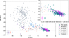 |
Fig. 5 Comparing the [Mo/Fe] disk abundances determined in this work (teal squares, as in Fig. 3) to those in previous studies in the disk (Mishenina et al. 2019, magenta downward pointing triangles) and the halo (Peterson 2013; Roederer et al. 2014a; Hansen et al. 2014; Spite et al. 2018, blue pluses, grey diamonds, coral triangles, purple crosses, respectively). This is also indicated in the lower right legend. The smaller upper rightmost plot shows a zoomed in portion of the higher metallicity region in the larger leftmost plot. The typical uncertainties reported in the studies are indicated in the lower left corner of both plots. The grey dashed lines that go through [0, 0] indicate the solar value, which we have normalised to A(Fe) = 7.45 (Grevesse et al. 2007) and A(Mo) =1.88 (Grevesse et al. 2015). |
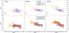 |
Fig. 6 [Mo/Fe] over [Fe/H] for the thick disk (yellow), thin disk (blue), and bulge (red) stars seen in the middle panels. The number of stars in each population is marked in the legend of the scatter plot (upper). The running mean (lower) is calculated using a box size of 10 (thick), 20 (thin), and 7 (bulge) stars and plotted with a 1σ deviation. We note that for the bulge, we only use stars with a spectra of >20 S/N to produce the running mean. We compare this to the s-process element Ce (left) and r-process element Eu (right) from Forsberg et al. (2019). The typical uncertainties are indicated in the lower right corner of the plots (red for bulge, grey for disk). The grey dashed lines that go through [0, 0] indicate the solar value, which we have normalised to A(Fe) = 7.45, A(Ce) = 1.70 (Grevesse et al. 2007), A(Mo) = 1.88, A(Eu) = 0.52 (Grevesse et al. 2015). The [Eu/Fe] values in Forsberg et al. (2019) are reported to likely be systematically too high, possibly originating from the systematic uncertainties in log(g) as reported in Paper I. Due to this, we lower the [Eu/Fe] abundances by 0.10 dex in this figure, such that the thin disk in [Eu/Fe] goes through the solar value. |
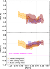 |
Fig. 7 Comparison of Mo with the s-process element Ce (top) and the r-process element Eu (bottom), for the running means of the populations, similarly to Fig. 6. We also plot the pure r-process line using the values in Prantzos et al. (2020; magenta). |
5 Discussion
Here, we first discuss the astrophysical sites for the s-, r-, and p-processes. We then compare with previous data of molybdenum, and end with a discussion of molybdenum as compared with other neutron-capture elements. Lastly, we briefly comment on the star HIP65028.
5.1 The neutron-capture and p-processes
As mentioned in Sect. 1, the origins of Mo are diverse, with stable isotopes originating from the s-, r-, and p-processes, or a combination of these. As for the two neutron-capture processes, the sites where these take place are constrained via the required neutron flux.
The s-process can be divided into two subprocesses, the main s-process and the weak s-process. The main s-process takes place in the interior of low- and intermediate asymptotic giant branch (AGB) stars in a 13C-pocket during the third dredge-up (see Karakas & Lattanzio 2014; Bisterzo et al. 2017, and references therein). This process is the main s-process producer of elements with A ≳ 90, such as cerium, which we compare our Mo abundances to. We refer the reader to Paper IV for a more in-depth description of the main s-process and its components.
The weak s-process requires higher temperatures and has the 22Ne(α, n)25Mg-reaction as a neutron source. As such, it takes place in the interior of massive stars with mass ≳8 M⊙. The weak s-process can produce trans-iron elements of 60 ≲ A ≲ 90, making its affect on the production of molybdenum-isotopes likely very small and close to negligible (Johnson & Bolte 2002; Pignatari et al. 2010; Prantzos et al. 2020).
However, some studies (e.g. Travaglio et al. 2004; Bisterzo et al. 2014, 2017) find that an additional process, Light Element Primary Process (LEPP), which is different from both the main s-process and the weak s-process, would be necessary to explain the abundances of Sr, Y, and Zr, as well as the s-only isotopes 96Mo and 130Xe. Nonetheless, the s-process has proven difficult to model, because of its dependence on a wide range of physical parameters, and the uncertainties on the yields (Cescutti & Matteucci 2022). The necessity for LEPP has also been questioned (see e.g. Cristallo et al. 2011, 2015; Trippella et al. 2016; Prantzos et al. 2020; Kobayashi et al. 2020); indeed it was deemed unnecessary when modifying parameters of Galactic chemical evolution models, such as the star formation rate, stellar yields, and varying the size of the 13C-pocket. Additionally, the rotation of massive stars has also been shown to have an affect on the amounts of s-process elements of A ≲ 90 being produced at low metallicities (Cescutti et al. 2013; Frischknecht et al. 2016; Limongi & Chieffi 2018). Therefore, the s-process contribution to molybdenum is believed to mainly come from the main s-process in AGB stars.
Given the AGB origin of main s-process elements, we expect these to have a trailing end at lower metallicities in abundance plots caused by the natural delay-time of AGB-stars. As AGB stars start to enrich the interstellar medium (ISM) with s-process elements, the abundance of these elements increases in newly formed stars, resulting in an increase in [s/Fe] before SNe type Ia start to enrich the ISM with iron, bringing the abundance trend down again (see e.g. observations in Mishenina et al. 2013; Battistini & Bensby 2016; Delgado Mena et al. 2017; Forsberg et al. 2019).
The r-process produces elements such as Eu, which we also compare with Mo. Given the high neutron flux required for the r-process, this is a production channel that works on very short timescales. The proposed production sites for the r-process are various SNe such as core-collapse, magneto-rotational, electron capture (CC, MR, EC, Woosley et al. 1994; Nishimura et al. 2006; Kobayashi et al. 2020; Wanajo et al. 2011) and neutron star mergers (NSMs; Freiburghaus et al. 1999; Matteucci et al. 2014). R-process ejecta was detected in observations of the electromagnetic signature from the NSM GW170817 (Abbott et al. 2017a,b; Kasen et al. 2017). However, Kobayashi et al. (2020) uses Galactochemical evolution models to show that NSMs are more or less negligible in the production of r-process elements, and point to MRSNe as the major contributor. Côté et al. (2019) and Skúladóttir & Salvadori (2020) point out the necessity for a combination of two sources with different delay-times in order to reproduce observed abundance trends – which is very similar to that of α-elements – in the Milky Way and some of the dwarf galaxies. In conclusion, there are still uncertainties as to the relative contributions from different sources. To determine the contribution from the suggested production sites is an active area of research, and having high-quality observational data for comparison with models is key in this continued effort.
The site of the p-process is even less well understood. Cameron (1957); Burbidge et al. (1957) suggested that it may take place in hydrogen-rich layers of SNe type II. The name ‘p-process’ refers to proton capture, but this is not necessarily always the case and there are several mechanisms and sites suggested as the cosmic origin for the p-isotopes, which we outline here (see also the review of Rauscher et al. 2013).
The γ-process is the photo-disintegration of heavy, neutron-rich isotopes that have already been created by means of neutron-capture processes, caused by highly energetic gamma-photons. (Woosley & Howard 1978; Arnould & Goriely 2003; Hayakawa et al. 2004; Pignatari et al. 2016). It has been proposed that the γ-process takes place in the explosive O/Ne-shell-burning stages of core-collapse SNe (Hoffman et al. 1994; Rayet et al. 1995; Pignatari et al. 2016; Nishimura et al. 2018; Travaglio et al. 2018), in pre-SNe stages (Ritter et al. 2018), or in type Ia SNe (Howard et al. 1991; Travaglio et al. 2011, 2015). As such, we expect the signature from these processes to be similar to the signatures for α- and iron-peak elements, which also originate from core-collapse SNe and type Ia SNe, respectively.
The v-process, which takes place during core-collapse SNe, could also be responsible for the production of p-isotopes. This process has been favoured among those put forward as giving rise to some of the lightest p-isotopes, including 92,94Mo (Woosley et al. 1990; Fröhlich et al. 2006).
The rapid proton-capture processes can be divided into three different processes, the rp-, pn-, and vp-process. The rapid proton capture takes place in proton-rich environments through (p,γ)-reactions (Schatz et al. 1998).
The rp-process is usually halted at isotopes with a combination of long half-lives and small proton-capture cross sections, causing ‘waiting points’ (Schatz et al. 2001). The rp-process has been suggested to be linked to the explosive hydrogen- and helium-burning on the surface of mass-accreting neutron stars (Schatz et al. 1998; Koike et al. 2004). These waiting points that halt the rp-process can be crossed either by the pn- or the vp-process. If there is a high density of neutrons, (n,p)-reactions can cross the waiting points, which is the pn-process. Otherwise, neutrons can be created through anti-neutrino interactions with protons, in  , which is the vp-process (Fröhlich et al. 2006).
The pn-process has been suggested to take place in a subclass of type Ia SNe which is the result of disruption of a sub-Chandrasekhar CO-white dwarf (WD) due to a thermonuclear runaway in He-rich accretion layers (Goriely et al. 2002). The site for the vp-process is thought to be either core-collapse SNe explosions or at accretion disks around compact objects (Fröhlich et al. 2006, 2017; Eichler et al. 2018).
In conclusion, there is a plethora of different mechanisms and sites that could produce the p-isotopes. By comparing to neutron-capture elements that dominate in the s- and r-process, the p-process might be disentangled from these.
Estimated uncertainties for Mo using the typical giant stars α–Boo and µ–Leo.
5.2 Comparison with previous work on molybdenum
As noted earlier, the disk [Mo/Fe]-trend in Mishenina et al. (2019) decreases at higher metallicities, whereas our disk trend decreases to a lesser degree. Furthermore, considering the separation of the thin and thick disk in Fig. 4, we see that the solar–[Mo/Fe] found at around [Fe/H]~ −0.4 in our data, corresponds to the thin disk, which is not observed in Mishenina et al. (2019). As such, our [Mo/Fe] trend with metallicity for the thin disk shows more of a trailing end at lower metallicities, which is typical for an s-process element that has a dominating enrichment from AGB stars at [Fe/H] ≳ −0.5, as discussed above.
As can be seen in Fig. 5, the cosmic scatter at [Fe/H] < −1.5 is extremely large, mostly based on the data from Roederer et al. (2014a). A similarly large spread at low metallicities is also seen for other neutron-capture elements, such as Eu (François et al. 2007; Frebel 2010; Cescutti et al. 2015) and ytterbium (Yb, Z = 70, also as published in Roederer et al. 2014a), whereas tighter trends are observed at higher metallicities (see e.g. Montelius et al. 2022, for Yb). The stochastic Galactochemical evolution models from Cescutti et al. (2015) can reproduce these observations and show that neutron-capture elements indeed have a large spread at lower metallicities. This is explained by the fact that at low metallicities, all neutron-capture elements in fact have an r-process origin, because the onset of s-process production of AGB has not yet taken place. The spread could be a signature of local r-process production, such as NSM, as discussed in Cescutti et al. (2015). This, in combination with the Galaxy not being well mixed, and indeed very low in Fe, could give rise to locally high [r-process/Fe], which is observed for [Mo/Fe].
It should be noted that the scatter at the lower metallicities, spanning the range [Mo/Fe] ~ 0–3.3 dex, mostly originates from the data of Roederer et al. (2014a), whereas the abundances of Peterson (2013); Hansen et al. (2014); Spite et al. (2018) are found within [Mo/Fe] ~ 0–1 dex. More abundances for these low-metallicity stars would be needed to further constrain the physical origin of this scatter for the r-process.
5.3 Comparison with other neutron-capture elements
We investigate the origin of Mo by comparing it to Ce which has a roughly 85% contribution from the s-process (Bisterzo et al. 2014; Prantzos et al. 2020) and to Eu which has a roughly 95% contribution from the r-process (Bisterzo et al. 2014; Prantzos et al. 2020), making these elements key representatives of these processes in the Galactic stellar populations. The abundance data for Ce and Eu in the disk and bulge come from Paper IV, and can be seen in Fig. 6, which reveals that the down-turning trailing end at lower metallicities is more prominent in [Ce/Fe] than in [Mo/Fe], which is expected from the theoretical origins of these elements. Moreover, both the thick disk and the bulge show decreasing [Mo/Fe]-trends with increasing metallicity – which is typical for an r-process element – due to the fast enrichment (see the models in Matteucci et al. 2014; Grisoni et al. 2020).
In [Eu/Fe], we observe a ‘knee’ or plateau in the thick disk at [Fe/H] ≤ −0.5, which is not observed for [Mo/Fe]. Indeed, [Mo/Fe] does not seem to plateau at all. However, more abundances at these metallicites are needed to further constrain this. With the combined data from Peterson (2013); Hansen et al. (2014); Roederer et al. (2014a) it does seem like [Mo/Fe] has a knee around [Fe/H] ~ −0.75 before the previously discussed increased scatter at low metallicities.
As previously stated in Paper IV, the general similarity between the thick disk and the bulge is high in [Ce, Eu/Fe], as seen in the running means of the abundances in the second row of Fig. 6, pointing to a similar star formation history of the populations. The [Ce,Eu/Fe] abundances in the running means are at some metallicities ~0.1 dex higher in the bulge than in the thick disk, however as the scatter is large in the bulge, we are unable to draw any robust conclusions.
It seems like the bulge is possibly enriched in [Mo/Fe] compared to the thick disk, especially at −0.5 < [Fe/H] < 0. However, we do note that the scatter is large for the bulge, and the following discussion is speculative based on the possible enrichment. As we do not see any difference between the stellar populations in either [Ce/Fe] or [Eu/Fe], the high [Mo/Fe] in the bulge could be linked to the p-process. In our previous studies, we found a possible enrichment in [V, Co, La/Fe] for the bulge, but these differences are not consistent with a single nucleosynthetic origin, meaning that, all elements considered, we cannot with confidence say that the bulge is distinguishable from the thick disk in the amount and rate of SNe type I and II. In turn, this means that the p-process sites linked to SNe type II and WD sources likely cannot produce the possible difference in the thick disk and bulge [Mo/Fe]. Of the suggested p-process sites, the one remaining is the rp-process, which is linked to burning on mass-accreting neutron stars (as discussed above, Schatz et al. 1998; Koike et al. 2004). However, there is no obvious reason why such events would be more common in the bulge, because either a high star formation rate or top-heavy initial mass function would make the bulge stand out in α-elements.
In order to further investigate the s- and r-process contribution to the origin of molybdenum, we also consider the abundance ratios of [Mo/Ce] and [Mo/Eu] over metallicity in Fig. 7. Here we only plot the running means so as to help with the interpretation of the trends. We also plot the so-called pure r-process line in the [Mo/Eu]-plot, which is calculated using the solar r-process contributions of the elements. The pure r-process is then the value of the r-process contribution in both elements, [r-process(Mo)/r-process(Eu)]. The closer the ratio is to the purer-process line, the more of the elements have a joint origin from the r-process (or rather are enriched by a source with similar time- and enrichment rate).
As all neutron-capture elements are produced by the r-process at lower metallicities, we can see that a greater proportion of Mo is produced by the r-process compared to Ce at low metallicities ≤−0.5. At [Fe/H] = −0.5, AGB stars (originating from low- to intermediate-mass stars) start to enrich the Galactic ISM with s-process elements, producing a higher fraction of Mo and Ce than the r-process. As a result, the [Mo/Ce] trend flattens out. Considering [Mo/Eu] in Fig. 7, we see an increase with increasing metallicities – again at [Fe/H] = −0.5 – due to the AGB enrichment, pointing at the s-process contribution to Mo. Below those metallicities, we observe a relative increase in Mo over Eu, which is linked to the lack of knee or plateau in Mo at these metallicities.
5.4 Comment on HIP65028
The star HIP65028 stands out as a Mo-enriched star in the thin disk, with [Mo/Fe] =0.68. Considering the values for other neutron-capture elements, [La/Fe] = 1.04, [Ce/Fe] = 0.96, [Eu/Fe] = 0.37 (Paper IV), we can conclude that this is a star enriched in s-process elements rather than r-process elements. This makes it a candidate Barium star, which could be investigated further by determining its C-abundance (which is usually high in Ba-stars) or by determining whether or not it has a strong variance in radial velocity measurements, which would indicate a binary companion. Usually these companions are WDs and stripped AGB-stars from where the carbon and s-process elements originate, and are too faint to be directly observed. Nonetheless, this also shows the high contribution from the s-process in creating Mo (~40 to 50% in Bisterzo et al. 2014; Prantzos et al. 2020, respectively) even at the low metallicities of [Fe/H] ~ −0.5 dex.
6 Conclusions
With this study, we continue our series of papers, determining high-quality abundances of bulge and disk stars using highresolution optical spectra with the aim of making a differential comparison between the stellar populations. We use the same type of stars (K-giants), the same spectral lines and atomic data, and the same method for analysing and determining the Mo abundances. By using the same set of spectral lines for all stars, we minimise the possible systematic uncertainties in the comparison of the bulge and the disk.
We determine Mo abundances for 35 bulge stars, which to the best of our knowledge is the largest sample of Mo abundances in bulge stars. We also determine Mo for 282 disk stars. With the previous sample of 183 disk stars from Mishenina et al. (2019), our sample significantly increases the Mo abundances determined at [Fe/H] ≳ −1.2. This allows us to both compare the bulge and disk stellar populations and investigate the cosmic origin of Mo.
Molybdenum has an interesting cosmic origin, being composed of a combination of seven stable isotopes, all with s-, r-, or p-process origin or a combination of these. We cannot determine the abundance of specific isotopes, but simply the overall abundance of Mo in our stellar populations. In comparison with other neutron-capture elements, such as Ce and Eu, we cannot exclude that Mo stands out in the bulge as compared to the thick disk. This could possibly be explained by the roughly 25% p-process origin of Mo (at solar metallicities). As such, the explanation to this possible difference between the bulge and thick disk could lie in understanding how and where these p-isotopes, namely 92,94Mo, form. The production site of p-isotopes is yet to be fully constrained, and although the scatter in our bulge sample is large, we speculate that an origin through mass-accreting neutron stars could possibly explain the seemingly high bulge abundances.
Acknowledgements
We thank Ross Church for insightful discussions about neutron-capture elements. We thank Lennart Lindegren for his expertise help in statistics. We also thank the anonymous referee for insightful comments that helped to improve this paper. R. F. and N. R. acknowledge support from the Royal Physiographic Society in Lund through the Stiftelse Walter Gyllenbergs fond and Märta och Erik Holmbergs donation. R. F.’s and A. J.’s research is supported by the Göran Gustafsson Foundation for Research in Natural Sciences and Medicine. A. J. acknowledges funding from the European Research Foundation (ERC Consolidator Grant 724687-PLANETESYS), the Knut and Alice Wallenberg Foundation (Wallenberg Academy Fellow Grant 2017.0287) and the Swedish Research Council (Project Grant 2018-04867). This work has made use of data from the European Space Agency (ESA) mission Gaia (https://www.cosmos.esa.int/gaia), processed by the Gaia Data Processing and Analysis Consortium (DPAC, https://www.cosmos.esa.int/web/gaia/dpac/consortium). Funding for the DPAC has been provided by national institutions, in particular the institutions participating in the Gaia Multilateral Agreement. Software: matplotlib (Hunter 2007), galpy (http://github.com/jobovy/galpy, Bovy 2015), astropy (Astropy Collaboration 2013).
Appendix A Supplementary data
Basic data for the observed solar neighbourhood giants. Coordinates and magnitudes are taken from the SIMBAD database, while the radial velocities are measured from the spectra.
Stellar parameters and determined abundances for observed solar neighbourhood giants.
Basic data for the observed bulge giants.
Stellar parameters and determined abundances for observed bulge giants.
References
- Abbott, B.P., Abbott, R., Abbott, T.D., et al. 2017a, Phys. Rev. Lett., 119, 161101 [CrossRef] [Google Scholar]
- Abbott, B.P., Abbott, R., Abbott, T.D., et al. 2017b, ApJ, 848, L12 [NASA ADS] [CrossRef] [Google Scholar]
- Allen, D.M., & Barbuy, B. 2006, A&A, 454, 917 [NASA ADS] [CrossRef] [EDP Sciences] [Google Scholar]
- Anders, F., Khalatyan, A., Queiroz, A.B.A., et al. 2022, A&A, 658, A91 [NASA ADS] [CrossRef] [EDP Sciences] [Google Scholar]
- Arnould, M., & Goriely, S. 2003, Phys. Rep., 384, 1 [Google Scholar]
- Astropy Collaboration (Robitaille, T.P., et al.) 2013, A&A, 558, A33 [NASA ADS] [CrossRef] [EDP Sciences] [Google Scholar]
- Barbuy, B., Chiappini, C., & Gerhard, O. 2018, ARA&A, 56, 223 [Google Scholar]
- Battistini, C., & Bensby, T. 2016, A&A, 586, A49 [NASA ADS] [CrossRef] [EDP Sciences] [Google Scholar]
- Bisterzo, S., Travaglio, C., Gallino, R., Wiescher, M., & Käppeler, F. 2014, ApJ, 787, 10 [NASA ADS] [CrossRef] [Google Scholar]
- Bisterzo, S., Travaglio, C., Wiescher, M., Käppeler, F., & Gallino, R. 2017, ApJ, 835, 97 [Google Scholar]
- Bovy, J. 2015, ApJS, 216, 29 [NASA ADS] [CrossRef] [Google Scholar]
- Budde, G., Burkhardt, C., Brennecka, G.A., et al. 2016, Earth Planet. Sci. Lett., 454, 293 [CrossRef] [Google Scholar]
- Budde, G., Burkhardt, C., & Kleine, T. 2019, Nat. Astron., 3, 736 [NASA ADS] [CrossRef] [Google Scholar]
- Burbidge, E.M., Burbidge, G.R., Fowler, W.A., & Hoyle, F. 1957, Rev. Mod. Phys., 29, 547 [CrossRef] [Google Scholar]
- Burkhardt, C., Kleine, T., Oberli, F., et al. 2011, Earth Planet. Sci. Lett., 312, 390 [CrossRef] [Google Scholar]
- Cameron, A.G.W. 1957, PASP, 69, 201 [NASA ADS] [CrossRef] [Google Scholar]
- Cardelli, J.A., Clayton, G.C., & Mathis, J.S. 1989, ApJ, 345, 245 [CrossRef] [Google Scholar]
- Cescutti, G., & Matteucci, F. 2022, Universe, 8, 173 [NASA ADS] [CrossRef] [Google Scholar]
- Cescutti, G., Chiappini, C., Hirschi, R., Meynet, G., & Frischknecht, U. 2013, A&A, 553, A51 [NASA ADS] [CrossRef] [EDP Sciences] [Google Scholar]
- Cescutti, G., Romano, D., Matteucci, F., Chiappini, C., & Hirschi, R. 2015, A&A, 577, A139 [NASA ADS] [CrossRef] [EDP Sciences] [Google Scholar]
- Côté, B., Eichler, M., Arcones, A., et al. 2019, ApJ, 875, 106 [Google Scholar]
- Cristallo, S., Piersanti, L., Straniero, O., et al. 2011, ApJS, 197, 17 [NASA ADS] [CrossRef] [Google Scholar]
- Cristallo, S., Straniero, O., Piersanti, L., & Gobrecht, D. 2015, ApJS, 219, 40 [Google Scholar]
- Delgado Mena, E., Tsantaki, M., Adibekyan, V.Z., et al. 2017, A&A, 606, A94 [NASA ADS] [CrossRef] [EDP Sciences] [Google Scholar]
- Di Matteo, P., Haywood, M., Gomez, A., et al. 2014, A&A, 567, A122 [NASA ADS] [CrossRef] [EDP Sciences] [Google Scholar]
- Eichler, M., Nakamura, K., Takiwaki, T., et al. 2018, J. Phys. G Nucl. Phys., 45, 014001 [NASA ADS] [CrossRef] [Google Scholar]
- Ek, M., Hunt, A.C., Lugaro, M., & Schönbächler, M. 2020, Nat. Astron., 4, 273 [NASA ADS] [CrossRef] [Google Scholar]
- Forsberg, R., Jönsson, H., Ryde, N., & Matteucci, F. 2019, A&A, 631, A113 [NASA ADS] [CrossRef] [EDP Sciences] [Google Scholar]
- François, P., Depagne, E., Hill, V., et al. 2007, A&A, 476, 935 [Google Scholar]
- Frebel, A. 2010, Astron. Nachr., 331, 474 [NASA ADS] [CrossRef] [Google Scholar]
- Freiburghaus, C., Rosswog, S., & Thielemann, F.K. 1999, ApJ, 525, L121 [NASA ADS] [CrossRef] [Google Scholar]
- Frischknecht, U., Hirschi, R., Pignatari, M., et al. 2016, MNRAS, 456, 1803 [Google Scholar]
- Fröhlich, C., Marünez-Pinedo, G., Liebendörfer, M., et al. 2006, Phys. Rev. Lett., 96, 142502 [CrossRef] [Google Scholar]
- Fröhlich, C., Hatcher, D., Perdikakis, G., & Nikas, S. 2017, in 14th International Symposium on Nuclei in the Cosmos (NIC2016), eds. S. Kubono, T. Kajino, S. Nishimura, T. Isobe, S. Nagataki, T. Shima, & Y. Takeda, 010505 [Google Scholar]
- Gaia Collaboration (Prusti, T., et al.) 2016, A&A, 595, A1 [NASA ADS] [CrossRef] [EDP Sciences] [Google Scholar]
- Gaia Collaboration (Brown, A.G.A., et al.) 2018, A&A, 616, A1 [NASA ADS] [CrossRef] [EDP Sciences] [Google Scholar]
- Gaia Collaboration (Brown, A.G.A., et al.) 2021, A&A, 649, A1 [NASA ADS] [CrossRef] [EDP Sciences] [Google Scholar]
- Gonzalez, O.A., & Gadotti, D. 2016, in Astrophysics and Space Science Library, Galactic Bulges, eds. E. Laurikainen, R. Peletier, & D. Gadotti, 418, 199 [NASA ADS] [CrossRef] [Google Scholar]
- Gonzalez, O.A., Rejkuba, M., Zoccali, M., et al. 2011, A&A, 530, A54 [NASA ADS] [CrossRef] [EDP Sciences] [Google Scholar]
- Gonzalez, O.A., Rejkuba, M., Zoccali, M., et al. 2012, A&A, 543, A13 [NASA ADS] [CrossRef] [EDP Sciences] [Google Scholar]
- Goriely, S., José, J., Hernanz, M., Rayet, M., & Arnould, M. 2002, A&A, 383, L27 [NASA ADS] [CrossRef] [EDP Sciences] [Google Scholar]
- Grevesse, N., Asplund, M., & Sauval, A.J. 2007, Space Sci. Rev., 130, 105 [NASA ADS] [CrossRef] [Google Scholar]
- Grevesse, N., Scott, P., Asplund, M., & Sauval, A.J. 2015, A&A, 573, A27 [NASA ADS] [CrossRef] [EDP Sciences] [Google Scholar]
- Grisoni, V., Cescutti, G., Matteucci, F., et al. 2020, MNRAS, 492, 2828 [Google Scholar]
- Gustafsson, B., Edvardsson, B., Eriksson, K., et al. 2008, A&A, 486, 951 [NASA ADS] [CrossRef] [EDP Sciences] [Google Scholar]
- Hansen, C.J., Andersen, A.C., & Christlieb, N. 2014, A&A, 568, A47 [NASA ADS] [CrossRef] [EDP Sciences] [Google Scholar]
- Hayakawa, T., Iwamoto, N., Shizuma, T., et al. 2004, Phys. Rev. Lett., 93, 161102 [NASA ADS] [CrossRef] [Google Scholar]
- Heiter, U., Jofré, P., Gustafsson, B., et al. 2015, A&A, 582, A49 [NASA ADS] [CrossRef] [EDP Sciences] [Google Scholar]
- Heiter, U., Lind, K., Bergemann, M., et al. 2021, A&A, 645, A106 [EDP Sciences] [Google Scholar]
- Hinkle, K., Wallace, L., & Livingston, W. 1995, PASP, 107, 1042 [Google Scholar]
- Hoffman, R.D., Woosley, S.E., Fuller, G.M., & Meyer, B.S. 1994, in American Astronomical Society Meeting Abstracts, 185, 33.09 [Google Scholar]
- Howard, W.M., Meyer, B.S., & Woosley, S.E. 1991, ApJ, 373, L5 [NASA ADS] [CrossRef] [Google Scholar]
- Hunter, J.D. 2007, Comput. Sci. Eng., 9, 90 [Google Scholar]
- Jofré, P., Heiter, U., Soubiran, C., et al. 2014, A&A, 564, A133 [NASA ADS] [CrossRef] [EDP Sciences] [Google Scholar]
- Jofré, P., Heiter, U., Soubiran, C., et al. 2015, A&A, 582, A81 [Google Scholar]
- Johnson, J.A., & Bolte, M. 2002, ApJ, 579, 616 [NASA ADS] [CrossRef] [Google Scholar]
- Johnson, C.I., McWilliam, A., & Rich, R.M. 2013, ApJ, 775, L27 [NASA ADS] [CrossRef] [Google Scholar]
- Jönsson, H., Ryde, N., Nordlander, T., et al. 2017a, A&A, 598, A100 [NASA ADS] [CrossRef] [EDP Sciences] [Google Scholar]
- Jönsson, H., Ryde, N., Schultheis, M., & Zoccali, M. 2017b, A&A, 600, A2 [NASA ADS] [CrossRef] [EDP Sciences] [Google Scholar]
- Karakas, A.I., & Lattanzio, J.C. 2014, PASA, 31, e030 [NASA ADS] [CrossRef] [Google Scholar]
- Kasen, D., Metzger, B., Barnes, J., Quataert, E., & Ramirez-Ruiz, E. 2017, Nature, 551, 80 [Google Scholar]
- Kobayashi, C., Karakas, A.I., & Lugaro, M. 2020, ApJ, 900, 179 [NASA ADS] [CrossRef] [Google Scholar]
- Koike, O., Hashimoto, M.-a., Kuromizu, R., & Fujimoto, S.-I. 2004, ApJ, 603, 242 [NASA ADS] [CrossRef] [Google Scholar]
- Lecureur, A., Hill, V., Zoccali, M., et al. 2007, A&A, 465, 799 [NASA ADS] [CrossRef] [EDP Sciences] [Google Scholar]
- Limongi, M., & Chieffi, A. 2018, ApJS, 237, 13 [NASA ADS] [CrossRef] [Google Scholar]
- Lind, K., Bergemann, M., & Asplund, M. 2012, MNRAS, 427, 50 [Google Scholar]
- Lomaeva, M., Jönsson, H., Ryde, N., Schultheis, M., & Thorsbro, B. 2019, A&A, 625, A141 [NASA ADS] [CrossRef] [EDP Sciences] [Google Scholar]
- Lugaro, M., Pignatari, M., Ott, U., et al. 2016, Proc. Natl. Acad. Sci. U.S.A., 113, 907 [NASA ADS] [CrossRef] [Google Scholar]
- Matteucci, F., & Brocato, E. 1990, ApJ, 365, 539 [CrossRef] [Google Scholar]
- Matteucci, F., Romano, D., Arcones, A., Korobkin, O., & Rosswog, S. 2014, MNRAS, 438, 2177 [Google Scholar]
- McMillan, P.J. 2018, RNAAS, 2, 51 [NASA ADS] [Google Scholar]
- McWilliam, A. 2016, PASA, 33, e040 [NASA ADS] [CrossRef] [Google Scholar]
- Meléndez, J., Asplund, M., Alves-Brito, A., et al. 2008, A&A, 484, L21 [NASA ADS] [CrossRef] [EDP Sciences] [Google Scholar]
- Mishenina, T.V., Pignatari, M., Korotin, S.A., et al. 2013, A&A, 552, A128 [NASA ADS] [CrossRef] [EDP Sciences] [Google Scholar]
- Mishenina, T., Pignatari, M., Gorbaneva, T., et al. 2019, MNRAS, 489, 1697 [NASA ADS] [CrossRef] [Google Scholar]
- Mishenina, T., Shereta, E., Pignatari, M et al. 2020, J. Phys. Stud., 24, N3 [CrossRef] [Google Scholar]
- Montelius, M., Forsberg, R., Ryde, N., et al. 2022, A&A, 665, A135 [NASA ADS] [CrossRef] [EDP Sciences] [Google Scholar]
- Ness, M., Freeman, K., Athanassoula, E., et al. 2012, ApJ, 756, 22 [NASA ADS] [CrossRef] [Google Scholar]
- Nishimura, S., Kotake, K., Hashimoto, M.-A., et al. 2006, ApJ, 642, 410 [Google Scholar]
- Nishimura, N., Rauscher, T., Hirschi, R., et al. 2018, MNRAS, 474, 3133 [NASA ADS] [CrossRef] [Google Scholar]
- Overbeek, J.C., Friel, E.D., & Jacobson, H.R. 2016, ApJ, 824, 75 [NASA ADS] [CrossRef] [Google Scholar]
- Pedregosa, F., Varoquaux, G., Gramfort, A., et al. 2011, J. Mach. Learn. Res., 12, 2825 [Google Scholar]
- Peterson, R.C. 2011, ApJ, 742, 21 [NASA ADS] [CrossRef] [Google Scholar]
- Peterson, R.C. 2013, ApJ, 768, L13 [NASA ADS] [CrossRef] [Google Scholar]
- Petit, P., Louge, T., Théado, S., et al. 2014, PASP, 126, 469 [NASA ADS] [CrossRef] [Google Scholar]
- Pignatari, M., Gallino, R., Heil, M., et al. 2010, ApJ, 710, 1557 [Google Scholar]
- Pignatari, M., Göbel, K., Reifarth, R., & Travaglio, C. 2016, Int. J. Mod. Phys. E, 25, 1630003 [NASA ADS] [CrossRef] [Google Scholar]
- Piskunov, N., & Valenti, J.A. 2017, A&A, 597, A16 [NASA ADS] [CrossRef] [EDP Sciences] [Google Scholar]
- Prantzos, N., Abia, C., Cristallo, S., Limongi, M., & Chieffi, A. 2020, MNRAS, 491, 1832 [Google Scholar]
- Queiroz, A.B.A., Anders, F., Santiago, B.X., et al. 2018, MNRAS, 476, 2556 [NASA ADS] [CrossRef] [Google Scholar]
- Rauscher, T., Dauphas, N., Dillmann, I., et al. 2013, Rep. Progr. Phys., 76, 066201 [CrossRef] [Google Scholar]
- Rayet, M., Arnould, M., Hashimoto, M., Prantzos, N., & Nomoto, K. 1995, A&A, 298, 517 [Google Scholar]
- Ritter, C., Andrassy, R., Côté, B., et al. 2018, MNRAS, 474, L1 [NASA ADS] [CrossRef] [Google Scholar]
- Roederer, I.U., Marino, A.F., & Sneden, C. 2011, ApJ, 742, 37 [NASA ADS] [CrossRef] [Google Scholar]
- Roederer, I.U., Preston, G.W., Thompson, I.B., et al. 2014a, AJ, 147, 136 [NASA ADS] [CrossRef] [Google Scholar]
- Roederer, I.U., Schatz, H., Lawler, J.E., et al. 2014b, ApJ, 791, 32 [NASA ADS] [CrossRef] [Google Scholar]
- Roederer, I.U., Lawler, J.E., Den Hartog, E.A., et al. 2022, ApJS, 260, 27 [NASA ADS] [CrossRef] [Google Scholar]
- Roriz, M.P., Lugaro, M., Pereira, C.B., et al. 2021, MNRAS, 507, 1956 [NASA ADS] [CrossRef] [Google Scholar]
- Schatz, H., Aprahamian, A., Goerres, J., et al. 1998, Phys. Rep., 294, 167 [CrossRef] [Google Scholar]
- Schatz, H., Aprahamian, A., Barnard, V., et al. 2001, Phys. Rev. Lett., 86, 3471 [CrossRef] [PubMed] [Google Scholar]
- Shen, J., & Zheng, X.-W. 2020, Res. Astron. Astrophys., 20, 159 [CrossRef] [Google Scholar]
- Skuladottir, Ä., & Salvadori, S. 2020, A&A, 634, A2 [Google Scholar]
- Spite, F., Spite, M., Barbuy, B., et al. 2018, A&A, 611, A30 [NASA ADS] [CrossRef] [EDP Sciences] [Google Scholar]
- Telting, J.H., Avila, G., Buchhave, L., et al. 2014, Astron. Nachr., 335, 41 [NASA ADS] [CrossRef] [Google Scholar]
- Thygesen, A.O., Sbordone, L., Andrievsky, S., et al. 2014, A&A, 572, A108 [NASA ADS] [CrossRef] [EDP Sciences] [Google Scholar]
- Travaglio, C., Gallino, R., Arnone, E., et al. 2004, ApJ, 601, 864 [Google Scholar]
- Travaglio, C., Röpke, F.K., Gallino, R., & Hillebrandt, W. 2011, ApJ, 739, 93 [NASA ADS] [CrossRef] [Google Scholar]
- Travaglio, C., Gallino, R., Rauscher, T., Röpke, F.K., & Hillebrandt, W. 2015, ApJ, 799, 54 [CrossRef] [Google Scholar]
- Travaglio, C., Rauscher, T., Heger, A., Pignatari, M., & West, C. 2018, ApJ, 854, 18 [NASA ADS] [CrossRef] [Google Scholar]
- Trippella, O., Busso, M., Palmerini, S., Maiorca, E., & Nucci, M.C. 2016, ApJ, 818, 125 [NASA ADS] [CrossRef] [Google Scholar]
- Valenti, J.A., & Piskunov, N. 1996, A&AS, 118, 595 [NASA ADS] [CrossRef] [EDP Sciences] [Google Scholar]
- Van der Swaelmen, M., Barbuy, B., Hill, V., et al. 2016, A&A, 586, A1 [NASA ADS] [CrossRef] [EDP Sciences] [Google Scholar]
- Wanajo, S., Janka, H.-T., & Müller, B. 2011, ApJ, 726, L15 [NASA ADS] [CrossRef] [Google Scholar]
- Weiland, J.L., Arendt, R.G., Berriman, G.B., et al. 1994, ApJ, 425, L81 [NASA ADS] [CrossRef] [Google Scholar]
- Whaling, W., & Brault, J.W. 1988, Phys. Scr, 38, 707 [CrossRef] [Google Scholar]
- Woosley, S.E., & Howard, W.M. 1978, ApJS, 36, 285 [NASA ADS] [CrossRef] [Google Scholar]
- Woosley, S.E., Hartmann, D.H., Hoffman, R.D., & Haxton, W.C. 1990, ApJ, 356, 272 [NASA ADS] [CrossRef] [Google Scholar]
- Woosley, S.E., Wilson, J.R., Mathews, G.J., Hoffman, R.D., & Meyer, B.S. 1994, ApJ, 433, 229 [NASA ADS] [CrossRef] [Google Scholar]
- Zoccali, M., Lecureur, A., Barbuy, B., et al. 2006, A&A, 457, L1 [NASA ADS] [CrossRef] [EDP Sciences] [Google Scholar]
Available at marcs.astro.uu.se
All Tables
Basic data for the observed solar neighbourhood giants. Coordinates and magnitudes are taken from the SIMBAD database, while the radial velocities are measured from the spectra.
Stellar parameters and determined abundances for observed solar neighbourhood giants.
All Figures
|
Fig. 1 Map of the Galactic bulge showing the five analysed fields, B3, BW, B6, BL (using the naming convention in Lecureur et al. 2007), and SW. The dust extinction towards the bulge is taken from Gonzalez et al. (2011, 2012) and scaled to optical extinction (Cardelli et al. 1989). The scale saturates at AV = 2, which is the upper limit in the figure. The COBE/DIRBE contours of the Galactic bulge, in black, are from Weiland et al. (1994). |
| In the text | |
|
Fig. 2 Observed spectrum (black) for a disk star (top, Arcturus) and bulge star (bottom, B3–B8). Left: line mask placements for the Mo line marked in blue and the continuum placements in yellow. Right: synthetic spectra, either in teal (top, disk star Arcturus) or red (bottom, bulge star B3–B8). The estimated S/N of both spectra, 117 and 72 respectively, are indicated in the legend. We note that the wavelength region of the rightmost figures is zoomed in with respect to the leftmost figures. |
| In the text | |
|
Fig. 3 [Mo/Fe] vs [Fe/H] for the disk (teal) and the bulge (red) in this study. The typical uncertainties, as described in Sect. 4.3 are indicated in the lower right corner. The grey dashed lines that go through [0, 0] indicate the solar value, which we have normalised to A (Fe) = 7.45 (Grevesse et al. 2007) and A(Mo) = 1.88 (Grevesse et al. 2015). |
| In the text | |
|
Fig. 4 Comparison of the [Mo/Fe] thin (blue squares) and thick (orange triangles) disk abundances determined in this work with the thin (black crosses) and thick (green diamonds) disk in Mishenina et al. (2019). It should be noted that the 23 stars that we do not have kinematical data for have not been classified as either thin or thick disk, and can be seen as grey circles. The typical uncertainties are indicated in the lower left corner (this work in grey, Mishenina et al. 2019 in black). The grey dashed lines that go through [0, 0] indicate the solar value, which we have normalised to A(Fe) = 7.45 (Grevesse et al. 2007) and A(Mo) = 1.88 (Grevesse et al. 2015). The thin disk star at [Fe/H] = −0.55 with high molybdenum abundance of [Mo/Fe] = 0.68, HIP65028, is discussed at the end of Sect. 5. |
| In the text | |
|
Fig. 5 Comparing the [Mo/Fe] disk abundances determined in this work (teal squares, as in Fig. 3) to those in previous studies in the disk (Mishenina et al. 2019, magenta downward pointing triangles) and the halo (Peterson 2013; Roederer et al. 2014a; Hansen et al. 2014; Spite et al. 2018, blue pluses, grey diamonds, coral triangles, purple crosses, respectively). This is also indicated in the lower right legend. The smaller upper rightmost plot shows a zoomed in portion of the higher metallicity region in the larger leftmost plot. The typical uncertainties reported in the studies are indicated in the lower left corner of both plots. The grey dashed lines that go through [0, 0] indicate the solar value, which we have normalised to A(Fe) = 7.45 (Grevesse et al. 2007) and A(Mo) =1.88 (Grevesse et al. 2015). |
| In the text | |
|
Fig. 6 [Mo/Fe] over [Fe/H] for the thick disk (yellow), thin disk (blue), and bulge (red) stars seen in the middle panels. The number of stars in each population is marked in the legend of the scatter plot (upper). The running mean (lower) is calculated using a box size of 10 (thick), 20 (thin), and 7 (bulge) stars and plotted with a 1σ deviation. We note that for the bulge, we only use stars with a spectra of >20 S/N to produce the running mean. We compare this to the s-process element Ce (left) and r-process element Eu (right) from Forsberg et al. (2019). The typical uncertainties are indicated in the lower right corner of the plots (red for bulge, grey for disk). The grey dashed lines that go through [0, 0] indicate the solar value, which we have normalised to A(Fe) = 7.45, A(Ce) = 1.70 (Grevesse et al. 2007), A(Mo) = 1.88, A(Eu) = 0.52 (Grevesse et al. 2015). The [Eu/Fe] values in Forsberg et al. (2019) are reported to likely be systematically too high, possibly originating from the systematic uncertainties in log(g) as reported in Paper I. Due to this, we lower the [Eu/Fe] abundances by 0.10 dex in this figure, such that the thin disk in [Eu/Fe] goes through the solar value. |
| In the text | |
|
Fig. 7 Comparison of Mo with the s-process element Ce (top) and the r-process element Eu (bottom), for the running means of the populations, similarly to Fig. 6. We also plot the pure r-process line using the values in Prantzos et al. (2020; magenta). |
| In the text | |
Current usage metrics show cumulative count of Article Views (full-text article views including HTML views, PDF and ePub downloads, according to the available data) and Abstracts Views on Vision4Press platform.
Data correspond to usage on the plateform after 2015. The current usage metrics is available 48-96 hours after online publication and is updated daily on week days.
Initial download of the metrics may take a while.