| Issue |
A&A
Volume 668, December 2022
|
|
|---|---|---|
| Article Number | A167 | |
| Number of page(s) | 17 | |
| Section | Catalogs and data | |
| DOI | https://doi.org/10.1051/0004-6361/202244422 | |
| Published online | 19 December 2022 | |
Superflares on solar-like stars
A new method for identifying the true flare sources in photometric surveys★
1
Max-Planck-Institut für Sonnensystemforschung,
Justus-von-Liebig-Weg 3,
37077
Göttingen, Germany
e-mail: This email address is being protected from spambots. You need JavaScript enabled to view it.
2
Sodankylä Geophysical Observatory and Space Physics and Astronomy Research unit, University of Oulu,
90014
Oulu, Finland
3
School of Physics, University of New South Wales,
Sydney, NSW
2052, Australia
4
UNSW Data Science Hub, University of New South Wales,
Sydney, NSW
2052, Australia
5
Institut für Astrophysik, Georg-August-Universität Göttingen,
Göttingen, Germany
6
Center for Space Science, NYUAD Institute, New York University Abu Dhabi,
Abu Dhabi, UAE
Received:
5
July
2022
Accepted:
26
September
2022
Abstract
Context. Over the past years, thousands of stellar flares have been detected by harvesting data from large photometric surveys. These detections, however, do not account for potential sources of contamination such as background stars or small Solar System objects appearing in the same aperture as the primary target.
Aims. We present a new method for identifying the true flare sources in large photometric surveys using data from the Kepler mission as an illustrative example. The new method considers not only the brightness excess in the stellar light curves, but also the location of this excess in the pixel-level data.
Methods. Potential flares are identified in two steps. First, we search the light curves for at least two subsequent data points exceeding a 5σ threshold above the running mean. For these two cadences, we subtract the “quiet” stellar flux from the Kepler pixel data to obtain new images where the potential flare is the main light source. In the second step, we use a Bayesian approach to fit the point spread function of the instrument to determine the most likely location of the flux excess on the detector. We match this location with the position of the primary target and other stars from the Gaia DR2 catalog within a radius of 10 arcsec around the primary Kepler target. When the location of the flux excess and the target star coincide, we associate the event with a flare on the target star.
Results. We applied our method to 5862 main-sequence stars with near-solar effective temperatures. From the first step we found 2274 events exceeding the 5σ level in at least two consecutive points in the light curves. Applying the second step reduced this number to 342 superflares. Of these, 283 flares occurred on 178 target stars and 47 events are associated with fainter background stars; in 10 cases the flare location could not be distinguished between the target and a background star. We also present cases where flares were reported previously but our technique could not attribute them to the target star.
Conclusions. We conclude that identifying outliers in the light curves alone is insufficient to attribute them to stellar flares and that flares can only be uniquely attributed to a certain star when the instrument pixel-level data together with the point spread function are taken into account. As a consequence, previous flare statistics are likely contaminated by instrumental effects and unresolved astrophysical sources.
Key words: methods: data analysis / stars: solar-type / stars: flare / stars: activity
Full Table 2 is only available at the CDS via anonymous ftp to cdsarc.cds.unistra.fr (130.79.128.5) or via https://cdsarc.cds.unistra.fr/viz-bin/cat/J/A+A/668/A167
© V. Vasilyev et al. 2022
 Open Access article, published by EDP Sciences, under the terms of the Creative Commons Attribution License (https://creativecommons.org/licenses/by/4.0), which permits unrestricted use, distribution, and reproduction in any medium, provided the original work is properly cited.
This article is published in open access under the Subscribe-to-Open model.
Open access funding provided by Max Planck Society.
1 Introduction
Flares are highly energetic outbursts in the stellar atmosphere caused by the reconnection of magnetic field lines. These events can be detected over a broad wavelength range from radio waves to gamma rays (Benz & Güdel 2010). On the Sun, flares have been observed in gamma rays and X-rays (Ackermann et al. 2014; Lysenko et al. 2020), in the UV and in white light (see, e.g., Haisch et al. 1991; Benz & Güdel 2010; Hudson 2011; Kretzschmar 2011), and in the radio band (Bastian et al. 1998).
Before the era of space telescopes, stellar flares had been detected only for a few G-type stars (Schaefer et al. 2000). With the advent of large photometric surveys, in particular the Kepler mission, it became clear that flares are common on cool stars (Walkowicz et al. 2011; Maehara et al. 2012; Shibayama et al. 2013; Davenport 2016; Van Doorsselaere et al. 2017; Yang & Liu 2019; Günther et al. 2020; Ilin et al. 2021). In particular, it was shown that G-dwarfs can experience very energetic flares (termed superflares) with radiative energies up to 1036 erg (Maehara et al. 2012). This energy is several orders of magnitude higher than the radiative energies of solar flares, which are usually well below 1032 erg (Hudson 2011). The highest solar flare energy ever detected was ~4 × 1032 erg (Emslie et al. 2012).
The question of whether the Sun can also unleash a super-flare is of crucial importance since it might lead to devastating consequences for humanity. The solar record alone is not sufficient to answer this question. At present, the only way to understand whether the Sun has experienced superflares is to search for extreme solar energetic particle (SEP) events in the cosmogenic-isotope data (e.g., Usoskin 2017; Miyake et al. 2020). These events are thought to be associated with very energetic flares. Currently there are eight known extreme SEP events (five confirmed, three pending) that occurred during the 12 millennia of the Holocene geological epoch (Usoskin & Kovaltsov 2021; Brehm et al. 2021, 2022). However, the relation between superflares and extreme solar particle events is still highly controversial, given that they are based on different physical manifestations (visible electromagnetic emission vs. fluence of energetic particles, respectively; see, e.g., Usoskin 2017).
Another way to understand whether the Sun is capable of unleashing superflares is provided by the solar-stellar comparison. Studies of stellar superflares have been progressively focusing on stars similar to the Sun (i.e., stars with near-solar effective temperatures and rotation periods). Constraining these two parameters is important because they define the action of stellar dynamos, and consequently stellar magnetic activity (see, e.g., the review by Reiners 2012).
In one of the first studies based on Kepler data, Maehara et al. (2012) found 14 superflares on stars with near-solar effective temperatures Teff = 5600-6000 K and rotation periods, Prot, longer than 10 days; for comparison, the solar sidereal Carrington rotation period is 25.4 days. Maehara et al. (2012) concluded that these stars unleash superflares with energies higher than 1034 erg (X1000-class flare in solar terminology) once every 800 yr. However, most of the flaring stars studied by Maehara et al. (2012) rotate significantly faster than the Sun, so their results are not directly applicable to the Sun. Consequently, more recent studies have focused on slower rotators. For example, Notsu et al. (2019) used measurements of stellar rotational periods by McQuillan et al. (2014) to conclude that stars with near-solar Teff and Prot ~ 25 days should unleash superflares every 2000-3000 yr. A more recent analysis by Okamoto et al. (2021) concluded that the Sun can unleash X1000-class superflares once every 6000 yr.
Crucially, all previous estimates of flare occurrence rates on solar-like stars have been based on the analysis of stars with known rotation periods. At the same time it has been shown that if the Sun were observed by Kepler, it would most probably be classified as an inactive star with an unknown rotation period (Aigrain et al. 2015; Reinhold et al. 2020, 2021; Shapiro et al. 2020; Amazo-Gómez et al. 2020). As a result, studies focused on stars with known rotation periods exclude most of the stars truly similar to the Sun, which might bias the statistics of superflares toward more active stars (Reinhold et al. 2020).
In this context, we take a different data-based approach for correcting the bias introduced by stars with unknown rotation periods. Specifically, we consider a larger sample of stars, mostly following the approach of Reinhold et al. (2020). These authors studied the variability of main-sequence stars with near-solar effective temperatures and metallicities. The majority of these stars had unknown rotation periods, but showed photometric variabilities very similar to the Sun’s. This sample of solar-like stars is analyzed for flares here.
When comparing solar and stellar flare statistics, it is important to keep in mind that highly energetic events are extremely rare on truly solar-type stars. Thus, every single flare detection will have a big impact on the statistics. This calls for accurate and stable methods of flare identification in large stellar samples.
In stellar light curves flares are seen as sudden brightness increases, followed by an exponential decay that typically lasts for several hours. Thus, previous flare studies were based on searching for outliers in the photometric time series. This approach, however, does not account for the possibility of flares occurring on background stars or other sources of brightness variations in the telescope’s field of view. Here we present a new method that is based on a combined analysis of the Kepler stellar light curves, Kepler target pixel files, and the high-precision astrometric data from the Gaia mission. This combination of data allows us to determine the most probable location of the brightness increase on the detector, and thus to distinguish between flares on the target star and background stars unresolved by the survey telescope. The aim of this paper is to present this new approach and apply it to a large sample of solar-like stars to gain better statistics on their flare frequencies. A statistical analysis of the results and its implication for the Sun will be the subject of a follow-up paper.
2 Data
In our analysis, we use two different data products of the Kepler telescope: the target pixel file (TPF) and the resulting light curves. The TPF contains a series of images centered at the target star. The size (in pixels) of each image depends on the target star (with an image scale of 3.98 arcsec per pixel).
Owing to the optical system of the telescope, the target flux is distributed over several pixels. To extract the flux of the target star, different aperture masks have been tested to sum up the flux of individual pixels. Before this step, the TPF underwent procedures of cosmic-ray removal and background corrections to maximize the flux of the target star. For each exposure, the sum of the pixels in the aperture equals the simple aperture photometry (SAP) flux.
The Kepler light curves are one-dimensional time series with flux measurements of the target stars. These have been subject to various corrections for instrumental systematics (Stumpe et al. 2012, 2014; Smith et al. 2012). In this study we used the pre-search data conditioning (PDC-SAP) flux from the latest data release (DR25), for which most instrumental effects have been removed. We only used the Kepler long-cadence (LC) data products1 with a cadence of ∆t ≈ 29.4 min. Kepler data were released in 18 quarters (Q0-Q17), most of which cover ~90 days each (with the exception of Q0, Q1, and Q17, which span a shorter time). We analyzed all available light curves and target pixel files (TPF) from quarters 0–17 for the entire observing period from May 2009 to May 2013.
The target list that we test our method on is based on the sample of stars with near-solar effective temperatures studied by Reinhold et al. (2020). These authors selected Kepler stars brighter than 15th magnitude with effective temperatures in the range 5500 < Teff < 6000 K, surface gravities log g > 4.2, and metallicities in the range −2.0 < [Fe/H] < 0.5 dex, using the catalog of Mathur et al. (2017). Additionally, we use the Gaia-DR2 catalog2 (Gaia Collaboration 2018) to retrieve astrometric data such as target positions (right ascension and declination), and G-band magnitudes of all stars within a radius of 10 arcsec around each Kepler target. Furthermore, we computed Gaia absolute magnitudes to select only main-sequence stars confined between two isochrones in the Hertzsprung-Russell diagram (for details, see Fig. 1 in Reinhold et al. 2020). By cross-matching the selected targets in the Kepler and Gaia archives, we found 5862 Kepler stars matching the selection criteria.
3 Methods
To identify flares on the selected stars, we employed a two-step algorithm. First, we collected potential flare events by searching the stellar light curves for data points exceeding a certain threshold. This approach is similar to the methods applied in earlier studies, although with some modifications (Sect. 3.1). Second, we localized the position of each event on the detector by fitting the instrument’s point spread function (PSF). If the positions of the target star and the event coincide, we concluded that the flare is associated with the target star (Sect. 3.2). These two steps are described in detail below.
3.1 Searching for flares in the light curves
Our first goal is to find potential flare events in the light curves of the target stars and identify their time of occurrence. Several flare detection methods have been reported (e.g., Shibayama et al. 2013; Johnson et al. 2017; Ilin et al. 2021). Generally, these methods are based on removing any variability on rotational and longer timescales from the light curves and searching for outliers in the detrended time series. More recent methods often use a Bayesian approach (Pitkin et al. 2014; Günther et al. 2020) or a machine-learning approach (Vida & Roettenbacher 2018; Feinstein et al. 2020).
Here, we used a simple moving average filter with the width of M = 15 data points (i.e., ~7.5 h) to detrend the time series. This approach reaches its limits when the width of the window becomes comparable to the stellar rotation period. In this study, however, we analyze solar-like stars that either have rotation periods > 20 days, as measured previously (McQuillan et al. 2014), or do not yet have periods reported. This makes it unlikely that the target star has a very short period (≲ 1 day) because short periods are detected more easily, and would likely have been measured before. The choice of the optimal flare detection filter is beyond the scope of this study.
The running mean filter is sensitive to discontinuities that are often found in the Kepler light curves. To reduce their impact, we excluded M cadences on either side of all data gaps longer than ΔtM/4 ≈ 2 h. Next, we applied the running mean filter, subtracted the smoothed light curve from the original one, and obtained a detrended time series. We excluded the first and the last M cadences from the detrended light curve due to the edge effects of the running mean. The fraction of rejected data points is around 3.2%. However, we found that the detrended light curves contain bumps due to individual outliers in the original light curve. Their impact can be reduced by either excluding or replacing them in the original light curves before applying the running mean filter. First, we excluded 1% of points with the lowest and highest flux in the detrended time series and computed the standard deviation σ for the remaining time series. Second, we found outliers that are above the chosen threshold of 2.5σ, replaced them in the non-detrended light curves, and repeated the procedure described above.
We identified potential flare events in the detrended light curves using the following criteria: (i) the event consists of at least two consecutive data points above the threshold set to 5σ, and (ii) there are no data gaps within 1.5 h before and after these points. The first criterion is set to detect the most energetic flares with high statistical confidence. The second criterion reduces the risk that some outliers might be related to instrumental effects (e.g., an increased noise level around the gap and statistical uncertainties caused by missing data. The moment in time of the first data point above 5σ is considered the time when the flare starts, and we denote it tflare. Typically, after reaching the maximum, the flare flux exponentially decays and, in the end, the light curve reaches a level similar to that before the flare. In the descending phase, we define the endpoint of the flare as the time when the flare flux crosses the 1σ level again. This point is defined by linear interpolation between the last data point above and the following one below the 1 σ level. Consequently, the interval between the flare start and endpoints is defined as the flare duration, denoted δtflare.
Figure 1 shows an example of the flare search in the light curve for the star KIC 10011070. We found a potential flare at tflare = 415.62 days satisfying our criteria described above.
3.2 Localization of flares in the target pixel files
After identifying all the potential flare candidates in the light curves, we used the series of images around each potential event (i.e., the target pixel files) to localize the source of the brightness excess in the sky. As described in Sect. 2, the Kepler pipeline generates the light curves using photometric aperture masks. These masks define the pixels on the CCD over which the flux of a given target is summed for each cadence. Potentially, a much fainter background star (below the sensitivity of Kepler) may fall in the same aperture as the target star. A flare on such a background star might be detectable in the final light curve, but would be misinterpreted as a flare on the target star. To address this, we localize the observed flux excess on the detector and match this location with the positions of the target and potential background stars from the Gaia DR2 catalog.
When starlight passes the optical system of a telescope, it is spread over the detector by the point spread function (PSF). The PSF is often wider than the pixel size of the detector, and therefore the starlight is distributed over several pixels. The image of a target recorded on the detector, known as the pixel response function (PRF), is a combination of the true image of the object produced by the optical system and the detector sensitivity. Thus, a reconstruction of the position of a star on the image requires knowledge of the shape of the PRF for a given instrument. The PRF of the Kepler instrument is a combination of the optical PSF, the spacecraft pointing jitter, the module defocus, the CCD response function, and the electronic impulse response (for details, see Bryson et al. 2010 and Van Cleve & Caldwell 2016). Extraction of the photometry by fitting the PSF and PRF is called PSF fitting.
The flare localization is based on the following key points. For each potential flare event, we select a series of images (target pixel files) before and after tflare. These time intervals represent the quiet stellar flux in the absence of the flare. The flare creates an additional flux excess in addition to the quiet stellar flux in the pixels close to the center of the target star during tflare and the following cadences. Our aim is to remove the quiet stellar flux to obtain a new series of images where the flare is the main light source. Then we model the flare at each cadence as a point source with a given position and flux convolved with the Kepler PRF and use a Bayesian approach to find the most likely flare location. We describe each of these steps in detail below.
We denote the image of the target star taken at the time tk as F(tk) = {Fp(tk)}, where k is the cadence, p is the pixel index, and Fp(tk) is flux [e−s−1] in the pixel p. Let Nx and Ny be the number of columns and rows in the image, where x (column number) and y (raw number) are the coordinates of a pixel on the two-dimensional image. Let Npix = NxNy be the total number of pixels in the image and 1 ≤ p ≤ Npix. For a given flare, we select images within a time interval ∆T = 0.6 days centered at íflare for this analysis.
As described above, the image of the target star might also contain contaminant stars. We denote the total stellar flux of all stars in a given pixel p during the absence of flares (i.e., quiet stellar flux) as  . A flare with the flux f(tk) and coordinates (x(tk), y(tk)) at a certain cadence tk introduces an additional flux in the image pixels because its light is distributed by the PSF. The flux excess from the flare in each pixel ∆Fp(tk) is given by the expression
 (1)
(1)
where Sp is the PRF of the pixel p on the detector and δtflare is the duration of the flare. For solar-like stars, δtflare is typically on the order of a few hours (Schrijver et al. 2012). Thus, the model of an image with a flare can be written as
 (2)
(2)
where np (t) is the photon noise.
The first step is to estimate the quiet stellar flux  in each pixel during the flare. To this end, we select images in time windows t ∈ [tflare − ∆T/2, tflare) and t ∈ (tflare + δtflare, tflare + δtflare + ∆T/2], when the flare contribution is zero (i.e., ∆Fp(t) = 0). In these time intervals we model the stellar flux
  by a smooth function. Since the brightness does not change significantly on such small timescales, we chose a cubic polynomial to fit the pixel fluxes at the cadences before and after the flare. In Fig. 2, we show the individual pixel fluxes Fp(t) from a series of images of the target star KIC 10011070 around tflare = 415.62 days and the fitted model
  representing the quiet stellar flux.
To obtain a series of images containing only the flux excess from the flare, we subtracted the estimated quiet flux from the images. In addition, to avoid negative flux values in the image pixels, we added an artificial offset c(tk) to each image and also took it into account in the analysis
 (3)
(3)
The new set of flare images is given by the expression
 (4)
(4)
where  is a vector representing the new image and in each pixel p the flux [e−s−1] is
 (5)
(5)
In Fig. 3 we show a series of six images D(tk) around tflare for the target star KIC 10011070.
We introduce a model representing the data:
 (6)
(6)
Here b(t) is a parameter characterizing the offset that we have introduced in Eq. (3), and ∆Fp(t, x(t), y(t), f(t)) is the flux excess due to the flare given by Eq. (1). For a given cadence k, we define a vector of the model parameters Θk = {xk, yk, fk, bk}. We estimate them using a Bayesian formalism. The posterior probability distribution P(Θk|Dk) is the conditional probability of the parameter set Θk given the data Dk
 (7)
(7)
where P(Θk) is the prior probability ascribed to the set of parameters, P(Dk|Θk) is the likelihood function, and P(Θk|Dk) is the posterior probability; P(Dk) is a normalizing factor that can be ignored for our purposes.
We assume that photons and electron counts in pixels obey Poisson statistics. Therefore, we use the likelihood function in the form of the Poisson distribution:
 (8)
(8)
where λp(Θk) is the expected flux for the pth pixel given by the model:
 (9)
(9)
Taking into account the parameter independence, we can write the prior probability as the product
 (10)
(10)
where NΘ = 4 is the number of the fitted parameters. For the flare flux fk, we take the uniformly distributed prior
 (11)
(11)
where  , and u denotes the uniform distribution. For the flare location, we take the uniformly distributed priors
 (12)
(12)
and
 (13)
(13)
where xk,min and yk,min are the pixel coordinates of the bottom left corner of the image, and Ncol and Nrow are the number of columns and rows of the image.
For the offset, we take the Gaussian prior
 (14)
(14)
with the width ![Mathematical equation: $\tilde \sigma _{k,b}^2 = {\rm{Var}}\left[ {D\left( {{t_k}} \right)} \right]$](/articles/aa/full_html/2022/12/aa44422-22/aa44422-22-eq23.png) and the mean
and the mean
 (15)
(15)
Since we are analyzing the Kepler data, we use the PRF of the Kepler telescope, but we note that the proposed method can be adapted for any photometric survey with known PRF. We use the LIGHTKURVE package (Lightkurve Collaboration 2018) to compute theoretical pixel fluxes λp(xk,yk,fk) on an image assuming a point source with a given position (xk, yk) and flux fk.
We separately analyze two images D(tflare) and D(tflare + Δt). According to the given threshold, there is a flux excess above 5σ in the light curve for these two cadences. We use the Goodman & Weare affine invariant Markov chain Monte Carlo (MCMC) ensemble sampler EMCEE (Goodman & Weare 2010; Foreman-Mackey et al. 2013) to compute the marginalized probability functions. A vector with initial parameters we denote as  . The center of brightness of the image D(tk) we use as the initial flare position is
 (16)
(16)
and
 (17)
(17)
where (Xp, Yp) is the pth pixel center coordinates. The sum of the pixel fluxes is taken as an initial guess of the flare flux:
 (18)
(18)
The mean of the pixel fluxes is taken as an initial guess of the offset:
 (19)
(19)
From the MCMC fitting, we obtain the final marginalized probability distribution functions (PDFs) of the model parameters.
The implementation of the method performing the steps described above is available in PYTHON. We provide an open source package LOCALIZATION OF SUPERFLARE EVENTS (LOSE) on GitHub3.
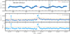 |
Fig. 1 Flare candidate detection in the light curve of star KIC 10011070 observed in quarter Q = 4. Top panel: original light curve (blue dots) and running mean (red line) calculated with a boxcar function averaging over 15 cadences. The vertical dashed lines indicate a period around a potential flare. Middle panel: zoom-in on the period around the flare candidate indicated in the top panel. The running mean is shown as a solid red line and the running 5σ threshold as a dash-dotted orange line. Bottom panel: detrended time series obtained by subtracting the running mean and normalizing by the standard deviation σ. The three consecutive data points in the middle clearly exceed the 5σ threshold. |
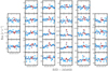 |
Fig. 2 Example of flux detrending in individual pixels for the star KIC 10011070 around the flare at tflare = 415.62 days. The blue dots are data points Fp(tk) used for the model of the flux variation in the absence of the flare |


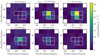 |
Fig. 3 Series of six D(tk) images with the flare at tflare = 415.62 days for the star KIC 10011070. The images of the subsequent cadences tflare = 415.62 and tflare = 415.64 days were used in the PSF fitting to localize the flare. Squares with white borders show the pixels of the aperture mask used to extract the light curve. |
3.3 Flare energies
For flares occurring on the target star, we measure the flare energy Eflare. We assume that the flare radiates as a blackbody with an effective temperature Tflare = 10 000 K (Hawley & Fisher 1992; Shibayama et al. 2013; Günther et al. 2020). The energy emitted by the flare each second is its bolometric luminosity
 (20)
(20)
where Aflare(t) is the area of the flare and Bλ(Tflare) the black-body spectrum integrated over all wavelengths. The total energy emitted by a flare is the integral of the luminosity over the flare duration
 (21)
(21)
The signal in each pixel of the CCD detector with a known transmission function ϕ(λ) is proportional to the number of photons falling onto the pixel during the exposure time Δt. Therefore, to obtain an estimate of the bolometric flare energy we have to convert the photon luminosity of the flare, denoted as Nflare, into the flare bolometric luminosity. The number of photons emitted by the flare at each time t in the passband ϕ(λ) is
 (22)
(22)
where c is the speed of light, and h is the Planck constant. Then the conversion factor α(Tflare) is given by the time-independent ratio
 (23)
(23)
Using Eqs. (20) and (22), we rewrite the ratio as
 (24)
(24)
In a similar way, we define a conversion factor α(T*) between the total number of emitted photons and the total emitted energy for the star as a whole
 (25)
(25)
where T* is the effective temperature and N* is the number of emitted photons of the star.
In the light curve the flare appears as a flux excess
 (26)
(26)
over the quiet stellar flux
 (27)
(27)
where r* is the distance from the observer to the star. Then, by combining Eqs. (24)-(27), we obtain the relationship between the bolometric luminosity of the flare and the observed light curve
 (28)
(28)
which we use with Eq. (21) to estimate the flare energy.
4 Results
4.1 Light curve analysis
From the flare search in the light curves (see Sect. 3.1), we obtained a list of flare candidates. In total, we found 2274 cases where at least two consecutive data points lie above the 5σ level in the detrended light curves. It is important to note that this number most likely also contains events not associated with the target star (e.g., cosmic rays, minor planets, residual instrumental effects). For each event that was detected in the light curve, we performed the PSF fitting (see Sect. 3.2).
4.2 PSF fitting of the flare
With the MCMC fitting, we obtained the 1D marginalized PDFs of the fit parameters. In Fig. 4 we show the marginalized 1D and 2D PDFs for the flare position (x(tk), y(tk)), the flare flux f(tk), and the offset b(tk) for the two subsequent cadences tk = tflare and tk = tflare + ∆t of the star KIC 10011070.
The position of the flare is constrained by drawing 2D confidence regions on the image. To do this we took into account that the sum of squares of two normally distributed random variables, x and y, have a chi-squared distribution with two degrees of freedom. Based on this, we drew 68%, 95%, and 99.9% confidence ellipses.
The PSF fitting returns the distributions of the most likely positions of the flare candidate for the two cadences. To match the location of the target (or any other star) and the confidence regions, we used the Gaia DR2 catalog (Gaia Collaboration 2018). We extracted the sky coordinates (α, δ) of all stars (including the target star) within a radius of 10 arcsec around the target star, and converted them into the pixel coordinates using the World Coordinate System (WCS) transformation. For both cadences, we checked whether a background or the target star lies within the 99.9% confidence level ellipse. To associate the potential flare with the star (target or background) we required that the star position is within the 99.9% confidence ellipse for both cadences.
In Fig. 5 we show the 2D confidence regions of the flare position for the target star KIC 10011070 as well as stars from the Gaia DR2 catalog on the two images D(tflare) and D(tflare + ∆t). In the regions of interest, we found three stars in the Gaia DR2 catalog: the target star and two fainter background stars. For both cadences, only the target star is located inside the 99.9% confidence region, whereas the two contaminant stars are far away from the estimated flare location. This leads us to conclude that the flare most likely happened on the target star.
It is important to note that we found cases where the confidence ellipse with the possible flare position is much bigger than the pixel size. These cases indicate that a proper solution in the MCMC runs cannot be found and that the observed signal is not associated with a flare. This is the case for the transits of minor planets, for example. Therefore, we retained only flare candidates when the possible flare position derived from the MCMC fit satisfied the following condition (for both cadences):
 (29)
(29)
Here a(tk) and g(tk) are the semi-axes of the 99.9% confidence level ellipse for tk = tflare and tk = tflare + ∆t. The threshold of two pixels is taken to reduce the number of cases when the ellipse size becomes comparable with the typical size of the photometric mask used to extract the light curve.
These two criteria, the location of a star within the 99.9% confidence region for both cadences and the sizes of the confidence ellipses given by Eq. (29), reduced the number of potential flares to 374. Next, for these events, we visually inspected the flare profiles in the light curves. Typically, the flare profile shows a steep increase of the flux followed by an exponential decay. However, we found several cases where the flare profile has a symmetrical shape with four or more points above the 1σ level. We associate these events with minor Solar System objects (see Sect. 4.5). In addition, we found several cases when the flare profile in the light curve has a long rising phase (≥ 1.5 h above the 1σ level) and a short descending phase (~30 min). We discarded such events from further analysis. The visual inspection further reduced the number of potential flares to 361.
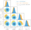 |
Fig. 4 Marginalized 1D and 2D PDFs of the model parameters used to fit the flare to the images D(tflare) and D(tflare + ∆t). The distributions derived by separately fitting the two cadences are shown in blue and orange (see inset). In the 2D plots, the different shades of blue and orange (dark to light) represent the 68%, 95%, and 99.9% confidence contours. The black dashed lines represent the pixel coordinates of the target star KIC 10011070 obtained by the coordinate transformation of the Gaia DR2 coordinates (α, δ). |
4.3 Distribution of events in time
A flare observed on a certain star happens independently from flares occurring on other stars. Thus, we would expect a uniform distribution of events in time. However, the presence of residual instrumental effects (i.e., an increase in the instrumental noise level in a short time interval) can produce outliers erroneously interpreted as flares. Therefore, we checked the temporal distribution of events detected in the light curve analysis (2274 events) and those after the flare localization using the PSF fitting method (361 events). These distributions are shown in Fig. 6. The distribution of events from the light curve analysis appears non-uniform. Around the times t = 1231 days and t = 1561 days, an anomalously large number of flare candidates have been detected. After the PSF fitting procedure and further analysis the peak at t = 1561 days vanished, but the peak at t = 1231 days persisted in the distribution. The inspection of the individual pixel fluxes showed that there was a systematic increase in the noise at that time. This increased noise level can be seen in the light curve and in the target pixel files. During the period t = 1231–1233 days we found 19 events, which were excluded from further analysis. Thus, our final list of flares associated with the target (or the background) star consists of 342 events.
4.4 Classification of events
Based on the results of the PSF fitting, we classified all events into the following groups: (i) flare on the target star, (ii) flare on a background star, (iii) flare that cannot be distinguished between the target and a background star, and (iv) (likely) not flares. In Table 1, we show the summary with the number of events detected in each step, and the number of flares in each group. The groups are described in detail below.
In Table 2, we list all detected flares and provide the Kepler ID of the target star (KIC), the Gaia DR2 ID, the time tflare of the first cadence above the 5σ threshold, the flare duration δtflare, and the stellar rotational period from McQuillan et al. (2014), if available. Additionally, we introduced a flag to distinguish between the three groups of flares. We set flag = 1 for flares detected on the target star, flag = 2 for flares detected on a background star, and flag = 3 if the flare cannot be distinguished between the target and background star. For the first group, we also provide the flare energy Eflare. For the last two cases, we provide the Gaia DR2 ID for the background star. A machine-readable version of the table is available at the CDS.
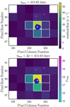 |
Fig. 5 Example of flare localization in the target pixel files for two subsequent cadences tflare (top) and tflare + ∆t (bottom). The star symbols are color-coded according to their apparent Gaia magnitude Gmag. The blue dots represent 1000 realizations of the flare position obtained from the MCMC fitting, and the red ellipses show the 68%, 95%, and 99.9% confidence regions. The squares with white borders show the pixels of the aperture mask used to extract the light curve. |
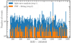 |
Fig. 6 Distribution of possible flare events in time after the analysis of the light curves (blue) and the PSF fitting of the flare images (orange). The bin width is 10 days. |
4.4.1 Flares on the target star
This group contains all events for which the target star lies within the 99.9% confidence ellipse for both cadences. In Fig. A.1, we show several examples with flares in the light curve and the images. Here we also include cases where both the target and a background star are contained within the ellipse at one cadence, but only the target star lies in the ellipse at the other cadence (see the top panel in Fig. A.1). In total, this group includes 283 flares on 178 solar-like stars; for 22 of these stars rotation periods were measured by McQuillan et al. (2014). For all 283 flares, we estimated the flare energy and its duration. In Table 2, we set flag = 1 for these events. Figures with light curves and results of the flare localization for these events can be found on the GitHub page of the project4.
Summary of detected events in the light curves and confirmed or rejected by the PSF fitting.
Catalog of detected flares.
4.4.2 Flares on background stars
This group consists of the events for which at least one background star lies within the 99.9% confidence ellipse and the target star is not located in the confidence ellipse for both cadences tflare and tflare + ∆t (see examples in Fig. B.1). In this group the largest number of flares (seven in total) is detected in the light curve data of KIC 7189661. However, according to the PSF fitting, these flares occurred on a faint background star (mG = 20.3) with the catalog number Gaia DR2 2102905052858466816. In total, we found 47 flares on 29 background stars in this group. In Table 2, we set flag = 2.
4.4.3 Flares indistinguishable between the target and a background star
This group refers to cases where the target star and the same background star are within the confidence ellipse for both cadences, tflare and tflare + ∆t. Thus, there is no possibility of uniquely assigning the flare to the target or the background star. We show several examples in Fig. C.1. In this group, we found 10 events on four stars. In Table 2, we set flag = 3.
4.5 Rejected cases
This group encompasses events that have at least two points above the 5σ threshold in the light curve and that belong to one of the following cases: (i) they do not satisfy the condition constraining the size of the confidence ellipse given by Eq. (29) for both cadences, (ii) the star (either target or background) within the confidence ellipse is not the same for both cadences, or (iii) the flare profiles with more than three points above the 5σ threshold in the light curve are symmetrical or have a longer rising phase compared to the descending phase. In Fig. D.1 we present several examples of such events.
Different physical processes can cause these types of events. Potentially, it can be a transit of a Solar System object across the image (see top panel Fig. D.1). Typically, such transits show a symmetrical shape in the light curve (i.e., the rising and declining phases look very similar). Owing to the fast proper motion of such objects relative to the stars, their reflected light is generally distributed over more pixels than the light from a single star (even during a single exposure). This effectively increases the size of the 2D confidence region (i.e., the size of the ellipse constraining the location of the event).
In addition, we found events that consist of two points above the 5σ threshold in the light curve but the confidence ellipses for the two subsequent cadences are located in two different pixels and the center of one ellipse lies outside of the other (see the middle panel in Fig. D.1). Possible sources of such events are subsequent cosmic ray hits. Cases were also found for which the location of the confidence ellipse does not change from one point in time to the other, but it does not overlap with any star (see the bottom panel in Fig. D.1). Such events might be caused by other astrophysical sources too faint to be detected by Gaia.
4.6 Comparison to Okamoto et al. (2021)
In this section, we compare our flare detections to those reported in the literature. Here, we focus on the latest flare catalog of solar-like stars provided by Okamoto et al. (2021; hereafter O2021), who conducted a statistical analysis of superflares on solar-like main-sequence stars. From the Kepler light curves, these authors detected 2344 flares on 256 stars with rotational periods in the range 1–40 days. Among these stars, there is a subsample of 16 solar-like stars with Teff = 5600–6000 K and Prot > 20 days (see Table 2 in O2021). To these stars, we applied our two-step algorithm described in Sect. 3 and found 38 flares. Interestingly, O2021 identified 29 flares. From our 38 flares, 22 flares coincide with those from O2021, and we identified 16 flares not listed by O2021. In addition, we applied our PSF fitting method to localize the 29 flares reported by O2021 using our PSF fitting method. As a result, seven events were rejected by the PSF fitting because the target star was not within the 99.9% confidence ellipse. In Fig. E.1 we show the light curves and images for these seven rejected cases.
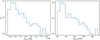 |
Fig. 7 Distribution of energies Eflare (left) and duration δtflare (right) of flares associated with the target star. |
4.7 Flare energies
Figure 7 shows the distribution of flare energies and durations for all events that we found to be associated with a target star. The flare energies are comparable with the estimates presented in the literature (Shibayama et al. 2013; Maehara et al. 2012; Okamoto et al. 2021). The highest flare energy measured in our sample is around Eflare ≈ 2 × 1035, which is roughly twice the maximum flare energy reported by O2021. The difference can potentially be due to the photon number to energy conversion factors, which has not been used in the literature. For stars from our sample with effective temperatures T, = 5500–6000 K, we estimate α(Tflare)/α(T*) ~ 1.5.
The proposed method for searching flares in the light curves, that is, the condition of having at least two subsequent data points above the 5σ threshold, sets the lower limit on the flare duration at δtmin > 30 min. Together with the assumption on the flare temperature, it also sets the lower limit of the flare energy, to which the method is sensitive.
5 Conclusions
In this work, we presented a new method for identifying the flare location in the target pixel files using the PSF fitting procedure. Previous flare detection methods were mostly based on the analysis of the light curves only. Our light curve analysis detected 2274 cases that could potentially be interpreted as a flare on the target star. However, the PSF fitting of the pixel data revealed that for more than 1900 of these cases the target star was not enclosed in the ellipses for both cadences tflare and tflare + ∆t. Thus, the flux excess detected in the light curve might arise from some other source of contamination, and cannot be uniquely attributed to the target star.
Even after the PSF fitting of the pixel data, not all detected flares can be associated with the target star. Of the 342 detected flares, only 283 actually happened on the 178 target stars, while the remaining cases either happened on a fainter background star or could not be uniquely attributed. Out of these 283 events, 45 flares happened on 22 stars for which rotational periods were measured by McQuillan et al. (2014), and 238 flares occurred on 156 solar-like stars with unknown rotation periods. However, we cannot completely exclude the possibility that some of these 156 stars were fast to medium rotation period stars (e.g., Prot < 20 days) that had been missed in the automated survey of McQuillan et al. (2014). This would, in turn, explain some of the flare detections. To test this hypothesis, further spectroscopic observations of all 178 flare stars are needed because previous spectroscopic characterizations of Sun-like superflare stars (e.g., Notsu et al. 2019) are scarce (see Appendix A in Okamoto et al. 2021).
To avoid false detections of flares on neighboring background stars, previous studies selected isolated stars (e.g., Okamoto et al. 2021). This criterion, however, often removes more than half of the stars from the initial target list (e.g., Shibayama et al. 2013 removed 70% from the initial sample). Our method does not require any sample reduction and allows us to detect flares on stars originally rejected in previous studies. That might help to improve statistics and provide a better estimate of the superflare occurrence frequency on Sun-like stars.
The results of our analysis lead us to conclude that the analysis of light curves alone is insufficient to associate outliers in the time series with flares on the target star. Thus, the flare statistics of previous studies might be contaminated by instrumental effects or unresolved background stars.
We emphasize that the method can, in principle, be applied to any photometric survey with known PSF. Thus, we expect the method to be useful for the analysis of the data from the TESS (Ricker et al. 2015) and upcoming PLATO missions (Rauer et al. 2016).
Acknowledgements
VV acknowledges support from the Max Planck Society under the grant “PLATO Science” and from the German Aerospace Center under “PLATO Data Center” grant 50OO1501. Part of this work was supported by the German Deutsche Forschungsgemeinschaft, DFG project number Ts 17/2-1. Part of this work has received funding from the European Research Council (ERC) under the European Union’s Horizon 2020 research and innovation program (grant agreement No. 715947). IU acknowledges support by the Academy of Finland (grant no. 321882 ESPERA), and inspiring discussions in the framework of the ISSI International team #510 SEESUP. L.G. acknowledges support from ERC Synergy Grant WHOLE SUN 810218. We also gratefully acknowledge use of the open-source codes MATPLOTLIB (Hunter 2007), NUMPY (van der Walt et al. 2011), SCIPY (Virtanen et al. 2020), and PYGTC (Bocquet & Carter 2016).
Appendix A Flare on the target star
 |
Fig. A.1 Two examples of flares associated with the target star. The symbols and colors are the same as in Fig. 5. |
Appendix B Flare on the background star
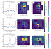 |
Fig. B.1 Three examples of flares occurring on background stars. The symbols and colors are the same as in Fig. 5. |
Appendix C Flares on target or background stars
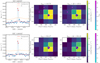 |
Fig. C.1 Two examples of events where the flare cannot be distinguished between the target and a background star. The symbols and colors are the same as in Fig. 5. |
Appendix D Rejected cases
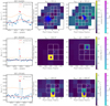 |
Fig. D.1 Rejected events. Top panels: Transit of a Solar System object across the image. Middle panels: Confidence ellipses of the two cadences (tflare and tflare + ∆t) are located in different pixels. Bottom panels: Confidence ellipses are at the same location for both cadences, but are not associated with any star in the Gaia DR2 catalog. |
Appendix E Rejected case from Okamoto et al. (2021)
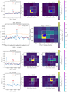 |
Fig. E.1 Seven Sun-like stars with flare detections reported by Okamoto et al. (2021) rejected by our method. Left panel: Light curve with the running mean (red line) and 5σ level (dash-dotted orange line) used to find flare candidates. The red dots show the cadences (tflare and tflare + Δt) for which the PSF fitting was performed. Middle and right panels: Residual images with the flare location and the 68%, 95%, and 99.9% confidence ellipses. For events that have only one data point above the 5σ level on the light curve, we performed the PSF fitting of the flare image only for that cadence. |
References
- Ackermann, M., Ajello, M., Albert, A., et al. 2014, ApJ, 787, 15 [NASA ADS] [CrossRef] [Google Scholar]
- Aigrain, S., Llama, J., Ceillier, T., et al. 2015, MNRAS, 450, 3211 [Google Scholar]
- Amazo-Gómez, E. M., Shapiro, A. I., Solanki, S. K., et al. 2020, A&A, 636, A69 [NASA ADS] [CrossRef] [EDP Sciences] [Google Scholar]
- Bastian, T. S., Benz, A. O., & Gary, D. E. 1998, ARA&A, 36, 131 [Google Scholar]
- Benz, A. O., & Güdel, M. 2010, ARA&A, 48, 241 [NASA ADS] [CrossRef] [Google Scholar]
- Bocquet, S., & Carter, F. W. 2016, J. Open Source Softw., 1, 46 [NASA ADS] [CrossRef] [Google Scholar]
- Brehm, N., Bayliss, A., Christl, M., et al. 2021, Nat. Geosc., 14, 10 [Google Scholar]
- Brehm, N., Christl, M., Knowles, T. D. J., et al. 2022, Nat. Commun., 13, 1196 [NASA ADS] [CrossRef] [Google Scholar]
- Bryson, S. T., Tenenbaum, P., Jenkins, J. M., et al. 2010, ApJ, 713, L97 [NASA ADS] [CrossRef] [Google Scholar]
- Davenport, J. R. A. 2016, ApJ, 829, 23 [Google Scholar]
- Emslie, A. G., Dennis, B. R., Shih, A. Y., et al. 2012, ApJ, 759, 71 [Google Scholar]
- Feinstein, A., Montet, B., & Ansdell, M. 2020, J. Open Source Softw., 5, 2347 [Google Scholar]
- Foreman-Mackey, D., Hogg, D. W., Lang, D., & Goodman, J. 2013, PASP, 125, 306 [Google Scholar]
- Gaia Collaboration 2018, VizieR Online Data Catalog: I/345 [Google Scholar]
- Gaia Collaboration (Brown, A. G. A., et al.) 2018, A&A, 616, A1 [NASA ADS] [CrossRef] [EDP Sciences] [Google Scholar]
- Goodman, J., & Weare, J. 2010, Commun. Appl. Math. Comput. Sci., 5, 65 [Google Scholar]
- Günther, M. N., Zhan, Z., Seager, S., et al. 2020, AJ, 159, 60 [Google Scholar]
- Haisch, B., Strong, K. T., & Rodono, M. 1991, ARA&A, 29, 275 [Google Scholar]
- Hawley, S. L., & Fisher, G. H. 1992, ApJS, 78, 565 [NASA ADS] [CrossRef] [Google Scholar]
- Hudson, H. S. 2011, Space Sci. Rev., 158, 5 [NASA ADS] [CrossRef] [Google Scholar]
- Hunter, J. D. 2007, Comput. Sci. Eng., 9, 90 [NASA ADS] [CrossRef] [Google Scholar]
- Ilin, E., Schmidt, S. J., Poppenhäger, K., et al. 2021, A&A, 645, A42 [NASA ADS] [CrossRef] [EDP Sciences] [Google Scholar]
- Johnson, E., Davenport, J. R. A., & Hawley, S. L. 2017, FBEYE: Analyzing Kepler light curves and validating flares, Astrophysics Source Code Library [record ascl:1712.011] [Google Scholar]
- Kretzschmar, M. 2011, A&A, 530, A84 [NASA ADS] [CrossRef] [EDP Sciences] [Google Scholar]
- Lightkurve Collaboration (Cardoso, J. V. D. M., et al.) 2018, Lightkurve: Kepler and TESS time series analysis in Python, Astrophysics Source Code Library [record ascl:1812.013] [Google Scholar]
- Lysenko, A. L., Frederiks, D. D., Fleishman, G. D., et al. 2020, Phys. Usp., 63, 818 [CrossRef] [Google Scholar]
- Maehara, H., Shibayama, T., Notsu, S., et al. 2012, Nature, 485, 478 [NASA ADS] [Google Scholar]
- Mathur, S., Huber, D., Batalha, N. M., et al. 2017, ApJS, 229, 30 [NASA ADS] [CrossRef] [Google Scholar]
- McQuillan, A., Mazeh, T., & Aigrain, S. 2014, ApJS, 211, 24 [Google Scholar]
- Miyake, F., Usoskin, I., & Poluianov, S., eds. 2020, Extreme Solar Particle Storms: The Hostile Sun (Bristol, UK: IOP Publishing) [Google Scholar]
- Notsu, Y., Maehara, H., Honda, S., et al. 2019, ApJ, 876, 58 [Google Scholar]
- Okamoto, S., Notsu, Y., Maehara, H., et al. 2021, ApJ, 906, 72 [NASA ADS] [CrossRef] [Google Scholar]
- Pitkin, M., Williams, D., Fletcher, L., & Grant, S. D. T. 2014, MNRAS, 445, 2268 [NASA ADS] [CrossRef] [Google Scholar]
- Rauer, H., Aerts, C., Cabrera, J., & PLATO Team. 2016, Astron. Nachr., 337, 961 [Google Scholar]
- Reiners, A. 2012, Living Rev. Sol. Phys., 9, 1 [Google Scholar]
- Reinhold, T., Shapiro, A. I., Solanki, S. K., et al. 2020, Science, 368, 518 [Google Scholar]
- Reinhold, T., Shapiro, A. I., Witzke, V., et al. 2021, ApJ, 908, L21 [NASA ADS] [CrossRef] [Google Scholar]
- Ricker, G. R., Winn, J. N., Vanderspek, R., et al. 2015, J. Astron. Telescopes Instrum. Syst., 1, 014003 [Google Scholar]
- Schaefer, B. E., King, J. R., & Deliyannis, C. P. 2000, ApJ, 529, 1026 [NASA ADS] [CrossRef] [Google Scholar]
- Schrijver, C. J., Beer, J., Baltensperger, U., et al. 2012, J. Geophys. Res. (Space Phys.), 117, A08103 [Google Scholar]
- Shapiro, A. I., Amazo-Gómez, E. M., Krivova, N. A., & Solanki, S. K. 2020, A&A, 633, A32 [NASA ADS] [CrossRef] [EDP Sciences] [Google Scholar]
- Shibayama, T., Maehara, H., Notsu, S., et al. 2013, ApJS, 209, 5 [Google Scholar]
- Smith, J. C., Stumpe, M. C., Van Cleve, J. E., et al. 2012, PASP, 124, 1000 [Google Scholar]
- Stumpe, M. C., Smith, J. C., Van Cleve, J. E., et al. 2012, PASP, 124, 985 [Google Scholar]
- Stumpe, M. C., Smith, J. C., Catanzarite, J. H., et al. 2014, PASP, 126, 100 [Google Scholar]
- Usoskin, I. G. 2017, Living Rev. Sol. Phys., 14, 3 [CrossRef] [Google Scholar]
- Usoskin, I., & Kovaltsov, G. 2021, Geophys. Res. Lett., 48, e94848 [NASA ADS] [CrossRef] [Google Scholar]
- Van Cleve, J. E., & Caldwell, D. A. 2016, Kepler Instrument Handbook, Kepler Science Document KSCI-19033-002 [Google Scholar]
- van der Walt, S., Colbert, S. C., & Varoquaux, G. 2011, Comput. Sci. Eng., 13, 22 [Google Scholar]
- Van Doorsselaere, T., Shariati, H., & Debosscher, J. 2017, ApJS, 232, 26 [NASA ADS] [CrossRef] [Google Scholar]
- Vida, K., & Roettenbacher, R. M. 2018, A&A, 616, A163 [NASA ADS] [CrossRef] [EDP Sciences] [Google Scholar]
- Virtanen, P., Gommers, R., Oliphant, T. E., et al. 2020, Nat. Methods, 17, 261 [Google Scholar]
- Walkowicz, L. M., Basri, G., Batalha, N., et al. 2011, AJ, 141, 50 [NASA ADS] [CrossRef] [Google Scholar]
- Yang, H., & Liu, J. 2019, ApJS, 241, 29 [NASA ADS] [CrossRef] [Google Scholar]
Kepler data products are available at https://archive.stsci.edu/missions-and-data/kepler
Data available at https://vizier.u-strasbg.fr/viz-bin/VizieR-3?-source=I/345/gaia2
All Tables
Summary of detected events in the light curves and confirmed or rejected by the PSF fitting.
All Figures
|
Fig. 1 Flare candidate detection in the light curve of star KIC 10011070 observed in quarter Q = 4. Top panel: original light curve (blue dots) and running mean (red line) calculated with a boxcar function averaging over 15 cadences. The vertical dashed lines indicate a period around a potential flare. Middle panel: zoom-in on the period around the flare candidate indicated in the top panel. The running mean is shown as a solid red line and the running 5σ threshold as a dash-dotted orange line. Bottom panel: detrended time series obtained by subtracting the running mean and normalizing by the standard deviation σ. The three consecutive data points in the middle clearly exceed the 5σ threshold. |
| In the text | |
|
Fig. 2 Example of flux detrending in individual pixels for the star KIC 10011070 around the flare at tflare = 415.62 days. The blue dots are data points Fp(tk) used for the model of the flux variation in the absence of the flare |
| In the text | |
|
Fig. 3 Series of six D(tk) images with the flare at tflare = 415.62 days for the star KIC 10011070. The images of the subsequent cadences tflare = 415.62 and tflare = 415.64 days were used in the PSF fitting to localize the flare. Squares with white borders show the pixels of the aperture mask used to extract the light curve. |
| In the text | |
|
Fig. 4 Marginalized 1D and 2D PDFs of the model parameters used to fit the flare to the images D(tflare) and D(tflare + ∆t). The distributions derived by separately fitting the two cadences are shown in blue and orange (see inset). In the 2D plots, the different shades of blue and orange (dark to light) represent the 68%, 95%, and 99.9% confidence contours. The black dashed lines represent the pixel coordinates of the target star KIC 10011070 obtained by the coordinate transformation of the Gaia DR2 coordinates (α, δ). |
| In the text | |
|
Fig. 5 Example of flare localization in the target pixel files for two subsequent cadences tflare (top) and tflare + ∆t (bottom). The star symbols are color-coded according to their apparent Gaia magnitude Gmag. The blue dots represent 1000 realizations of the flare position obtained from the MCMC fitting, and the red ellipses show the 68%, 95%, and 99.9% confidence regions. The squares with white borders show the pixels of the aperture mask used to extract the light curve. |
| In the text | |
|
Fig. 6 Distribution of possible flare events in time after the analysis of the light curves (blue) and the PSF fitting of the flare images (orange). The bin width is 10 days. |
| In the text | |
|
Fig. 7 Distribution of energies Eflare (left) and duration δtflare (right) of flares associated with the target star. |
| In the text | |
|
Fig. A.1 Two examples of flares associated with the target star. The symbols and colors are the same as in Fig. 5. |
| In the text | |
|
Fig. B.1 Three examples of flares occurring on background stars. The symbols and colors are the same as in Fig. 5. |
| In the text | |
|
Fig. C.1 Two examples of events where the flare cannot be distinguished between the target and a background star. The symbols and colors are the same as in Fig. 5. |
| In the text | |
|
Fig. D.1 Rejected events. Top panels: Transit of a Solar System object across the image. Middle panels: Confidence ellipses of the two cadences (tflare and tflare + ∆t) are located in different pixels. Bottom panels: Confidence ellipses are at the same location for both cadences, but are not associated with any star in the Gaia DR2 catalog. |
| In the text | |
|
Fig. E.1 Seven Sun-like stars with flare detections reported by Okamoto et al. (2021) rejected by our method. Left panel: Light curve with the running mean (red line) and 5σ level (dash-dotted orange line) used to find flare candidates. The red dots show the cadences (tflare and tflare + Δt) for which the PSF fitting was performed. Middle and right panels: Residual images with the flare location and the 68%, 95%, and 99.9% confidence ellipses. For events that have only one data point above the 5σ level on the light curve, we performed the PSF fitting of the flare image only for that cadence. |
| In the text | |
Current usage metrics show cumulative count of Article Views (full-text article views including HTML views, PDF and ePub downloads, according to the available data) and Abstracts Views on Vision4Press platform.
Data correspond to usage on the plateform after 2015. The current usage metrics is available 48-96 hours after online publication and is updated daily on week days.
Initial download of the metrics may take a while.