| Issue |
A&A
Volume 699, July 2025
|
|
|---|---|---|
| Article Number | A90 | |
| Number of page(s) | 13 | |
| Section | Stellar atmospheres | |
| DOI | https://doi.org/10.1051/0004-6361/202452867 | |
| Published online | 01 July 2025 | |
Observational signs of limited flare area variation and peak flare temperature estimations in main-sequence flaring stars
1
Astronomical Institute, University of Wrocław,
Kopernika 11,
51-622
Wrocław,
Poland
2
University of Wrocław, Centre of Scientific Excellence – Solar and Stellar Activity,
Kopernika 11,
51-622
Wrocław,
Poland
3
Astronomical Institute, Academy of Sciences of the Czech Republic,
25165
Ondřejov,
Czech Republic
4
Department of Physics and Astronomy, Shumen University “Episkop Konstantin Preslavski”,
115 Universitetska Str.,
9700
Shumen,
Bulgaria
★ Corresponding author: This email address is being protected from spambots. You need JavaScript enabled to view it.
Received:
4
November
2024
Accepted:
14
May
2025
Abstract
In the study of stellar flares, traditional method of calculating total energy emitted in the continuum assumes the emission originating from a narrow chromospheric condensation region with a constant temperature of 10 000 K and variable flare area. However, based on multicolor data from seven new flares observed in Białków and Shumen observatory and eight previously published flares observed on ten main-sequence stars (spectral types M5.5V to K5V – nine M-dwarfs and one K-dwarf) we show that flare areas had a relative change in the range of 10–61% (for more than half of the flares this value did not exceed 30%) throughout the events except for the impulsive phase, and had values starting from 50 ± 30 ppm to 300 ± 150 ppm for our new flares and from 380 ± 200 ppm to 7600 ± 3000 ppm from previously published flare data, while their temperature increased on average by the factor 2.5. The peak flare temperatures for our seven observed flares ranged from 5700 ± 450 K to 17 500 ± 10 050 K. Five of these flares had their temperatures estimated using the Johnson-Kron-Cousins B filter alongside TESS (Transiting Exoplanet Survey Satellite) data, one flare was analyzed using the SLOAN g′ and r′ bandpasses, and another was evaluated using both the SLOAN g′ and r′ bandpasses and TESS data. Using flare temperature and area data, along with the physical parameters of stars where the flares occurred, we developed a semiempirical grid that correlates a star’s effective temperature and flare amplitude in TESS data with the flare’s peak temperature. This allows interpolation of a flare’s peak temperature based on the star’s effective temperature (ranging from 2700 K to 4600 K) and flare amplitude from TESS observations. Applying this grid to 42 257 flares from TESS survey, we estimated peak flare temperatures between 5700 K and 38 300 K, with most flares showing peak blackbody temperatures around 11 100 ± 2400 K.
Key words: stars: activity / stars: flare / stars: late-type / stars: low-mass
© The Authors 2025
 Open Access article, published by EDP Sciences, under the terms of the Creative Commons Attribution License (https://creativecommons.org/licenses/by/4.0), which permits unrestricted use, distribution, and reproduction in any medium, provided the original work is properly cited.
This article is published in open access under the Subscribe to Open model. This email address is being protected from spambots. You need JavaScript enabled to view it. to support open access publication.
1 Introduction
Flares are random and unpredictable events on the surfaces of stars, characterized by the intense release of magnetic energy in the outer stellar atmosphere. These flares produce a range of observable effects across various wavelengths, emitting energy in both emission lines and the continuum. The continuum, especially from the far-ultraviolet (FUV) to the optical range, dominates the energy output. During the peak of most flares, a few percent of the total energy is in the emission lines, which can rise to 20% during the gradual decay phase (Kowalski et al. 2013). In certain cases, line emission can contribute up to 50% of the total flare energy (Hawley et al. 2007).
On the Sun, our ability to see the detailed surface observations allows us to study flares frequently and in great detail, providing significant insights into flare processes and their consequences. The total energy emitted by solar nanoflares and microflares, observed in X-ray on very short timescales, can be as low as 1021–1024 erg (impulsive events occur at a frequency of ∼ 25 events per minute with a typicalpp lifetime of ∼ ten minutes) (Preś et al. 2005; Upendran et al. 2022). However, this energy can reach levels typical of a solar flares visible in white light, ranging from 1029 erg to approximately 1032–1033 erg (Shibata & Yokoyama 2002; Cliver & Dietrich 2013), with durations spanning from several minutes to several hours. To date, no solar flare having energy exceeding 1033 erg, have been observed. For other active stars, although it is not possible to observe flares with the same level of detail, we are still able, under favorable conditions, to estimate their location on the surface of the star (Ilin et al. 2021; Bicz et al. 2024). Stellar flares can be over a thousand times more intense than solar flares, with durations ranging from minutes to several hours (Pietras et al. 2022). In extraordinary cases, a flare can last over a day (Bicz et al. 2024).
The continuum emission of stellar flares is often modeled as blackbody radiation with a fixed temperature of 10 000 K, while the flare’s area changes over time (Shibayama et al. 2013; Namekata et al. 2017; Günther et al. 2020; Bicz et al. 2022; Pietras et al. 2022). In this model, the flare area is described as a unified radiating structure, where white-light ribbons and cool loops are not distinct entities but interconnected components of a single composite system on the star’s surface. It is important to note that, during a flare, temperature evolves over time similarly to solar observations, as shown in studies by Gershberg & Shakhovskaya (1972); Kunkel (1975); Mochnacki & Zirin (1980), and others. Hawley & Fisher (1992) modeled atmospheric responses to flare energy, finding that conductive heating balanced optically thin cooling in the transition region.
However, discrepancies in emission ratios and line profiles indicated additional heating in the upper chromosphere. Observed flare continuum spectra, resembling blackbody radiation (8500– 9500 K), were attributed to photospheric reprocessing of upper chromospheric UV-EUV emissions. Hawley et al. (1995) analyzed optical and coronal data, finding strong evidence of a stellar “Neupert effect,” which supports chromospheric evaporation models. They further argued that the spatial correlation between white-light and hard X-ray emissions in solar flares, along with the identification of hard X-rays as nonthermal bremsstrahlung from accelerated electrons, indicates that flare heating on dMe stars follows the same electron precipitation mechanism observed on the Sun. Their study of a large EUV flare emphasized the role of coronal loop length in flare energetics, further extending the solar flare model to stellar environments. Zhilyaev et al. (2007) studied EV Lac flares, confirming high-frequency oscillations tied to hydrogen plasma state transitions. Peaks matched blackbody temperatures of 17 000– 22 000 K, with flares covering ∼ 1% of the stellar disk. Kowalski et al. (2013) explored M-dwarf flares, showing that electron beams primarily heated the chromosphere. Numerical models highlighted wave interactions and localized heating, predicting NUV and optical continua at temperatures ≥ 12 000 K, consistent with observed flare properties. The total energy of the flare is determined by its blackbody temperature and the evolving flare area. Although, the actual blackbody temperatures of superflares are still uncertain. For M-dwarf flares, continuum temperatures typically range between 9000 and 14 000 K (Kowalski et al. 2013), but in some cases, they can surpass 40 000 K (Robinson et al. 2005; Kowalski & Allred 2018; Froning et al. 2019). Substantial temperature variations are observed during stellar flares as the energy source propagates from the lower chromosphere into the coronal regions (Livshits et al. 1981; Fisher et al. 1985b,a; Fisher 1989). Such a process is called chromospheric evaporation. During a solar or stellar flare near a magnetic reconnection area, local plasma escapes as a two-directional stream along the magnetic flux rope. The escaping plasma is heated, and electrons are accelerated to non-thermal energies. Both thermal conduction and the accelerated electrons can deliver a high-energy flux to the dense chromosphere, which responds with explosive heating and expansion. As a result, hot plasma flows upward and quickly fills the newly formed flare loops (Fisher et al. 1985a; Falewicz 2014; Dudík et al. 2016; Yang et al. 2021).
In this study, we measured the evolution of blackbody temperatures and areas for seven flares using multi-color photometry. Five of these flares were observed at by Białków Observatory (Poland) at approximately one-minute intervals and the Transiting Exoplanet Survey Satellite (TESS; Ricker et al. 2014) at both two-minute and 20-second intervals. The remaining two flares were observed by TESS and the Shumen Observatory (Bulgaria). Eight additional flares from Howard et al. (2020) were incorporated to enhance the statistical analysis. By utilizing the blackbody temperature evolution data of these flares, we calculated the flare area evolution for eight additional events.
Because multi-color observations of stellar flares are limited we tried to prepare an improved procedure that allows for the analysis of stellar flares using single-channel observations, comparable to those conducted with multiple channels. Using calculated temperature and derived area evolution of the analyzed flares we were able to create a grid, allowing us to interpolate the peak temperature of any flare that occurs on a main-sequence flaring star. To do so we need the amplitude of the flare calculated from TESS observations and the effective temperature of the star. This method works for the stars with effective temperatures in the range from 2700 K up to 4600 K.
The paper is organized as follows. In Sect. 2, we describe the simultaneous flare observations and host star properties. In Sect. 3, we describe our method for estimating the flare’s temperature and area changes, as well as our calculations of the flare’s energy. In Sect. 4, we present the results and propose a new method for estimating the peak temperature of a flare. In Sect. 5, we summarize and discuss the results.
2 Observations
2.1 Białków observations
The observational data from Białków Observatory of the University of Wrocław, Poland were obtained using a 60 cm Cassegrain telescope equipped with an Andor Tech. DW432-BV backilluminated CCD camera. This setup provides a field of view of 13′ × 12′ in the B and V bandpasses of the Johnson-Kron-Cousins photometric system with approximately 70 s cadence for each bandpass. Flare temperatures were estimated using the B/TESS flux ratio to avoid the effect of noise in the V-band photometry. To check if these temperatures were accurate enough, we compared the observed V-band signal with the signal expected from the calculated temperature and flare area. The results matched very well, with differences usually smaller than two standard deviations.
During the nights of October 6/7 and 19/20, 2022, five flares were observed on the active M-dwarf star EV Lacertae at Białków Observatory. These flares have numbers from one to five in this paper (see Fig. 1). EV Lacertae (EV Lac) is classified as an M4Ve (Lépine et al. 2013) flaring star with an effective temperature of approximately 3300 ± 200 K, radius of 0.34 ± 0.01 R⊙, and mass of 0.32 ± 0.02 M⊙ (MAST1 catalog2). The star is approximately 5.05 pc away from the Sun (Gaia Collaboration 2021). EV Lac has rotation period of 4.359 days (Paudel et al. 2021). The surface of EV Lac hosts extensive starspots capable of covering a significant portion of the stellar surface (Jeffers et al. 2022; Ikuta et al. 2023), and it experiences superflares with energies significantly exceeding those of the strongest solar flares (Ikuta et al. 2023).
2.2 Shumen observations
The data from Shumen Observatory, Bulgaria were collected using a 40 cm reflector Meade LX200ACF equipped with an FLI PL09000 CCD camera (Kjurkchieva et al. 2020). This configuration provides a 30′ × 30′ field of view in the g′, r′, and i′ bandpasses of the Sloan photometric system. Due to the absence of significant signal increases in the i′ bandpasses during the flare, we limited our analysis to the g′ and r′ bandpasses.
On the night of July 4/5, 2022, a flare on V374 Pegasi was observed (Flare 6, see Fig. 2). V374 Peg is a fully convective M3.5Ve dwarf star (Morin et al. 2008b) situated at a distance of 9.1 pc. It has a mass of 0.29 ± 0.02 M⊙, a radius of 0.31 ± 0.01 R⊙, and an effective temperature of 3200 ± 200 K (MAST catalog). The estimated rotation period for V374 Peg is 0.4457572 ± 0.0000002 days (Bicz et al. 2022). We observed the star with exposure times equal to 25 s in g′ and 20 s in r′. Only this star had observations in i′ bandpass. The surface of V374 Peg can be spotted over five percent (Bicz et al. 2022), the spots can be stable on a one-year timescale (Morin et al. 2008a), and energies of the flares on this star reach over 1033 erg (Bicz et al. 2022).
Additionally, on the night of August 2/3, 2022, a flare on the star GJ 1243 was observed at Shumen Observatory (Flare 7, see Fig. 3). GJ 1243 is a fully convective M4.0V dwarf star (Lépine et al. 2013) located at a distance of 11.95 pc. The star has a mass of 0.24 ± 0.02 M⊙, a radius of 0.27 ± 0.01 R⊙, and an effective temperature of 3200 ± 200 K (MAST catalog). Its rotation period is 0.59260 ± 0.00021 days (Davenport et al. 2015). The star had exposure times equal to 20 s in g′ and 15 s in r′. GJ 1243 is a subject of many studies due to its enormous flaring activity (Davenport et al. 2020; Bicz et al. 2022) and the presence of very long-living spots on its surface (Davenport et al. 2014; Bicz et al. 2022). The spotedness on this star varies around a few percent and flares have energies that exceed the Carrington Event (Davenport et al. 2014; Bicz et al. 2022).
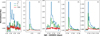 |
Fig. 1 Normalized light curves of five flares of EV Lac in three different passbands. The blue, green, and red curves represent the B-band, V-band made in Białków Observatory, and the 20 s TESS observations, respectively. The panels are labelled with the flare number (Table 1). |
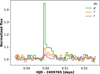 |
Fig. 2 Normalized light curve of the Flare 6 of V374 Peg in three band-passes g′, r′, and the i′ (labeled). Observations were made in Shumen Observatory. |
2.3 TESS observations
TESS is a space telescope launched in April 2018 and placed in a highly elliptical orbit with a period of 13.7 days. The primary objective of the mission is to conduct continuous observations of a substantial portion of the celestial sphere that is divided into sectors. The satellite monitors target stars with a two-minute cadence (short cadence) and a 20-second cadence (fast cadence) over a monitoring period of approximately 27 days in each sector. Light curves can also be obtained from the Full Frame Images.
The five flares observed on EV Lac at Białków Observatory were also detected by TESS during Sector 57. Additionally, the flare on GJ 1243 observed at Shumen Observatory was captured by TESS in Sector 54. For these six flares, both 20-second and two-minute cadence data from TESS observations were available. The comprehensive comparison of all conducted observations can be seen in Table 1.
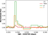 |
Fig. 3 Normalized light curve of the Flare 7 of GJ 1243, observed in two bandpasses, g′ and r′ (labeled), at Shumen Observatory, along with the 20 s normalized light curve from TESS (labeled). |
2.4 Flare data from Howard et al. (2020)
To increase our sample of flares we used the continuum temperature evolution data from eight flares analyzed by Howard et al. (2020) using observations from TESS and Evryscope (Law et al. 2016; Ratzloff et al. 2019). We selected the data based on acceptable measurement errors to ensure reliable results. These flares are highlighted in the two bottom panels of Fig. 4 and are labeled (a), (b), (d), (f), (g), and (h) in Fig. 5 of the mentioned paper. Table 2 shows in detail on which star each flare occurred, the time of occurrence, and the peak temperature (average temperature within the full width at half maximum as defined in Howard et al. 2020). Additionally, the first column of Table 2 shows the flare’s number in this paper.
Informations about observations of the flares analyzed in this paper.
Information about the flares from Howard et al. (2020) used in the present paper.
2.5 Cadence of observations
Observations in multiple filters were conducted alternately, meaning they are not simultaneous. As a result, it was necessary to align both datasets on a common timeline. To achieve this, a linear interpolation of observation epochs, brightness values, and their uncertainties was performed for data from both observatories (Shumen and Białków) to match the observation times of TESS. Similarly, the Evryscope observations from Howard et al. (2020) were interpolated onto the TESS timeline. As an alternative approach we could compare the closest data points from Shumen or Białków observations with the nearest TESS observations, assuming that the physical conditions of events separated by less than a minute remain synchronous. However, this method would have increased the uncertainty in temperature estimations and introduced distortions, either overestimating or underestimating the values depending on the flare phase. We chose linear interpolation as it eliminates temporal differences between observations from different observatories. Moreover, linear interpolation does not significantly alter the profiles of most observed events, which often last for a considerable duration. Near the peak of the flare’s emission, this interpolation method may slightly underestimate the maximum temperature. However, for time differences of only a few seconds, the underestimation of temperature remains negligible.
3 Methods
3.1 Flare temperature and area estimation
The method we used closely follows the approach outlined by Hawley et al. (2003). We defined the temperature of a flare (Tflare) as the effective temperature deduced from the flare’s spectral characteristics. The TESS bandpass lies in the tail of the Planck curve, resulting in minimal energy excess within the TESS bandpass for high temperatures (temperatures higher than 10 000 K). However, other bandpasses used in observations fall in the bluer region of the Planck curve, leading to higher flare amplitudes at elevated temperatures. Some of the spectroscopic observations of flares show a non-negligible Balmer jump, but focusing the energy estimates on the optical continuum that provides a dominant contribution, we considered the blackbody temperature obtained from that continuum. Both spectral observations as well as RHD simulations show, for very strong electron-beam fluxes, that the Paschen optical continuum can be well fitted by the Planck function, while the Balmer continuum is present apparently due to non-homogeneous temperature and density structure of the chromospheric condensation (see Kowalski 2024). Note that at lower densities of the chromospheric condensations the Balmer jump appears naturally even in the case of isothermal slabs (e.g., Heinzel 2024). Moreover, the ultraviolet tail of the B filter from the Białków Observatory that we used exhibits a minimal response to the Balmer jump, approximately 0.4%. The temperature estimation process is as follows:
We used synthetic spectra from the PHOENIX library (Husser et al. 2013) to obtain the radiation spectrum for a star with the specified effective temperature, metallicity, and surface gravity over the wavelength range encompassing the entire filter in which the flare was observed.
We multiplied the spectrum by the response functions for the given filters and integrate over all wavelengths to determine the star’s flux in each bandpass and the energy emitted by the flare at each instant.
By estimating the energy surpluses in multiple band-passes, we calculated the flare’s area and temperature at each measurement point by solving the equations Lflare = AflareBλ(Tflare) for the set of bandpasses where Aflare is the area of the flare. To solve the equation we used the assumption that the flare’s area does not vary much in different bandpasses thus we may solve the system of equations for Tflare and Aflare separately (Durán & Kleint 2020; Howard et al. 2020).
Using the temporal temperature evolution data from Howard et al. (2020) as a basis, we analyzed the changes in the flare area in time using the light curve observed by the TESS satellite. To perform calculations we assumed that the spectrum of white-light flares can be modeled as blackbody radiation, which is consistent with optically thick Pashen continuum (Heinzel 2024). The combined luminosity (L) from both the flare and the remaining stellar surface can be expressed as:
![Mathematical equation: \[L = \left( {{A_{{\rm{star\;}}}} - {A_{{\rm{flare\;}}}}} \right){F_{{\rm{star\;}}}} + {A_{{\rm{flare\;}}}}{F_{{\rm{flare\;}}}},\]](/articles/aa/full_html/2025/07/aa52867-24/aa52867-24-eq1.png) (1)
where Fflare, Aflare, Fstar, and Astar represent the fluxes and areas of the stellar disk and the flare, respectively. The flux of the star is described by:
(1)
where Fflare, Aflare, Fstar, and Astar represent the fluxes and areas of the stellar disk and the flare, respectively. The flux of the star is described by:
![Mathematical equation: \[{L_{{\rm{star\;}}}} = {A_{{\rm{star\;}}}}{F_{{\rm{star\;}}}}.\]](/articles/aa/full_html/2025/07/aa52867-24/aa52867-24-eq2.png) (2)
(2)
The normalized light curve of the star (C) is then given by:
![Mathematical equation: \[C = \frac{L}{{{L_{{\rm{star\;}}}}}} = \frac{{\left( {{A_{{\rm{star\;}}}} - {A_{{\rm{flare\;}}}}} \right){F_{{\rm{star\;}}}} + {A_{{\rm{flare\;}}}}{F_{{\rm{flare\;}}}}}}{{{A_{{\rm{star\;}}}}{F_{{\rm{star\;}}}}}}.\]](/articles/aa/full_html/2025/07/aa52867-24/aa52867-24-eq3.png) (3)
(3)
This formula can be rewritten to express the area of the flaring region as:
![Mathematical equation: \[{A_{{\rm{flare\;}}}} = \frac{{(C - 1){A_{{\rm{star\;}}}}{F_{{\rm{star\;}}}}}}{{{F_{{\rm{flare\;}}}} - {F_{{\rm{star\;}}}}}}.\]](/articles/aa/full_html/2025/07/aa52867-24/aa52867-24-eq4.png) (4)
(4)
The above relation can naturally be rewritten as:
![Mathematical equation: \[{A_{{\rm{flare\;}}}} = \frac{{(C - 1)\pi R_{{\rm{star\;}}}^2\mathop \smallint \nolimits_{{\lambda _1}}^{{\lambda _2}} {S_\lambda }{B_\lambda }\left( {{T_{{\rm{star\;}}}}} \right)d\lambda }}{{\mathop \smallint \nolimits_{{\lambda _1}}^{{\lambda _2}} {S_\lambda }{B_\lambda }\left( {{T_{{\rm{flare\;}}}}} \right)d\lambda - \mathop \smallint \nolimits_{{\lambda _1}}^{{\lambda _2}} {S_\lambda }{B_\lambda }\left( {{T_{{\rm{star\;}}}}} \right)d\lambda }},\]](/articles/aa/full_html/2025/07/aa52867-24/aa52867-24-eq5.png) (5)
where λ is the wavelength, Bλ(T) is the Planck function, Tstar and Rstar are the star’s effective temperature and radius, respectively, and S λ is the instrument’s response function. This equation made it possible for us to estimate how the flare area evolves throughout the event, provided the temporal temperature evolution and photometric data.
(5)
where λ is the wavelength, Bλ(T) is the Planck function, Tstar and Rstar are the star’s effective temperature and radius, respectively, and S λ is the instrument’s response function. This equation made it possible for us to estimate how the flare area evolves throughout the event, provided the temporal temperature evolution and photometric data.
3.2 Observational estimation of flare peak temperatures
Available flare observations allowed us to estimate the flare temperature only at the observational points relative to a chosen filter. As a result, we often lacked an exact measurement of the peak signal, since the maximum phase is short-lived. By fitting a theoretical flare profile to observations, we were able to infer where this maximum should occur.
We fitted the Wrocław flare profile (Gryciuk et al. 2017; Bicz et al. 2022; Pietras et al. 2022) to the photometric data using an evolutionary algorithm code3 (Bicz et al. 2024) to model the temperature evolution of the analyzed flares. For all flares except Flare 6, we utilized the TESS light curve, selected for its high data cadence and low noise (this flare was not observed by TESS). For Flare 6, we chose the g′ light curve (represented by the green curve in Fig. 2). Each flare was subjected to 10 000 fits to achieve the best possible match. By considering possible peak temperatures – from the star’s effective temperature up to 60 000 K – along with the estimated flare surface from multicolor photometry we can estimate the theoretical temperature evolution of the flare using fitted profile by solving the rewritten Eq. (5):
![Mathematical equation: \[\mathop \smallint \limits_{{\lambda _1}}^{{\lambda _2}} {S_\lambda }{B_\lambda }\left( {{T_{{\rm{flare\;}}}}} \right)d\lambda = \left( {\frac{{(C - 1)\pi R_{{\rm{star\;}}}^2}}{{{A_{{\rm{flare\;}}}}}} + 1} \right)\mathop \smallint \limits_{{\lambda _1}}^{{\lambda _2}} {S_\lambda }{B_\lambda }\left( {{T_{{\rm{star\;}}}}} \right)d\lambda .\]](/articles/aa/full_html/2025/07/aa52867-24/aa52867-24-eq6.png) (6)
(6)
Using this grid of solutions for a given range of peak temperatures we can find the best fit to the temperature evolution data (estimated as in Sect. 3.1). This allowed us to deduce the flare’s peak temperature. We used the normalized χ2 statistics to evaluate the goodness of fit.
3.3 Flare energy estimation
The bolometric energy of each flare (Eflare) can be calculated using the temporal temperature evolution of the flare (Tflare) with the corresponding flaring area (Aflare). This calculation involves summing the energy emitted at different time intervals (Δt) across the entire electromagnetic spectrum, assuming that the flare’s spectrum can be modeled as blackbody radiation of a given temperature Tflare. The expression for Eflare (Method I) is given by:
![Mathematical equation: \[{E_{{\rm{flare\;}}}} = \mathop \sum \limits_{i = 0}^{n - 1} \left( {{A_{{\rm{flare}}\;,i}}{\rm{\Delta }}{t_i}\pi \mathop \smallint \limits_0^{ + \infty } {B_\lambda }\left( {{T_{{\rm{flare}}\;,i}}} \right)d\lambda } \right),\]](/articles/aa/full_html/2025/07/aa52867-24/aa52867-24-eq7.png) (7)
where Bλ is the Planck function and n is the total number of measurement points captured during the flare. To further compare the results of Method I, we used the approach outlined by Shibayama et al. (2013) (referred to as Method II), which assumes a constant flare temperature of 10 000K while allowing the flare area to vary. Method II also assumes that the flaring region is substantially smaller than the total stellar surface.
(7)
where Bλ is the Planck function and n is the total number of measurement points captured during the flare. To further compare the results of Method I, we used the approach outlined by Shibayama et al. (2013) (referred to as Method II), which assumes a constant flare temperature of 10 000K while allowing the flare area to vary. Method II also assumes that the flaring region is substantially smaller than the total stellar surface.
4 Results
4.1 Evolution of observational areas and temperatures of flares
We found that the estimated peak blackbody temperatures of our newly observed flares ranged from 5700 K to 17 500 K (Table 3). To validate our flare peak temperature estimation method, we applied it to the eight flares analyzed from Howard et al. (2020). The peak flare temperatures for the flares from Howard et al. (2020) estimated by us ranged from 7000 to 31 500 K, and all our peak temperature estimates for these flares are consistent with their results within the margin of error. Among our newly observed flares, two had peak temperatures below 8000 K, four fell within the 8000–14 000 K range (the upper limit of the typical range quoted in Kowalski et al. 2013), and one exceeded 14 000 K. The bolometric energies of our seven flares, estimated using Method I, ranged from (2.0 ± 1.3) × 1031 erg to (1.9 ± 0.9) × 1032 erg, while for the flares from Howard et al. (2020), they ranged from (3.3 ± 1.7) × 1031 erg to (1.2 ± 0.5) × 1032 erg. All seven flares observed in our study had energies below the superflare threshold (1033 erg). In contrast, all flares that we used in this paper from Howard et al. (2020) exceeded this threshold, except for Flares 9 and 14. The bolometric energies derived using Method II ranged from (1.9 ± 0.6) × 1031 erg to (1.9 ± 0.5) × 1035 erg for our seven observed flares and from (3.3 ± 1.7) × 1031 erg to (1.2 ± 0.5) ×1035 erg for the flares analyzed by Howard et al. (2020).
For the Flares 1, 6, and 10, Method II produced significantly different energies, with differences ranging from the energy 0.65 times lower for Flare 10 to the energy approximately four times higher for Flare 1. The average flare areas ranged from 50 ± 30 ppm4 for Flare 6 to 300 ± 150 ppm for Flare 7 among our seven newly observed flares, and from 380 ± 200 ppm for Flare 14 to 7600 ± 3000 ppm for Flare 8 in the data from Howard et al. (2020). Only one flare had an area smaller than 100 ppm; nine flares had areas between 100 ppm and 1000 ppm, and five flares had areas exceeding 1000 ppm. To improve the clarity of the flare area results and reduce tshe influence of the very large observational uncertainties an adaptive rebinning was performed on the data. Data points were grouped into different-sized bins depending on the associated uncertainties: in regions that had small uncertainties, few bins were grouped together, while larger bins were used in areas of higher uncertainty. Again, data points where the relative uncertainty became larger than the value itself had their bin size further increased to receive uncertainty lower than the rebinned value (see Fig. 4). During the rebinning process the data uncertainties were used as weights. This rebinning allowed us to estimate that the flare area varies, on average, by approximately 50% of the mean flare area value. For almost all of the analyzed flares we remark the lack of significant changes of the estimated flare area. Some variations are noted for the rise phases of the Flares 1, 8, and 11. When the flares pass to the gradual phase, these changes vanish. It is worth noting that although it is physically plausible that a flare develops during the rise phase, this phase of the evolution is hard to control with the time cadence achieved in our observations. We performed statistical tests to evaluate the validity of the assumption that these areas remain constant. The fourth column in the Table 3 lists the value of possible changes of the flare area estimated from the linear fit to the rebinned data relative to their weighted average. This value usually does not exceed the level of 30%. Only for the Flares 5 and 7 it reaches the value of over 50%. We also performed F-test to compare the residual variances for the two assumptions: first that the area is constant and second that it shows an important trend. The fifth column lists the probability of the assumption that there are no significant changes in the estimated area. As one can see this probability is high for almost all analyzed flares. The only outstanding event is Flare 7, but even here this probability is not low enough to statistically reject the assumption of the constant area model. The temperature and area evolution for selected flares are illustrated in Fig. 4. Table 3 presents the detailed values of bolometric energies (see also Fig. 5), estimated areas, and peak flare temperatures, along with their uncertainties. Notably, only two flares (1 and 7) required a single-component Wrocław flare profile for a good fit, while the remaining flares required a two-component Wrocław flare profile that is consistent with the previously obtained results (see Bicz et al. 2022 and Pietras et al. 2022 for more details).
Peak temperatures, mean areas, and F-test results for constancy of flare area over time.
4.2 Semiempirical grid for estimating the peak flare temperatures of main-sequence stars
Most of the stellar flares are observed only in one bandpass. This includes huge database of flares recorded by Kepler and TESS missions. For such events, it is not possible to apply the analysis outlined in this paper. To make it possible we must estimate the flare temperature at its peak. In this study, we aim to develop a method for making reasonable predictions of the peak temperatures of the flares basing on the stars’ spectral classification and the observed flares’ magnitudes. The observed flux from a flare is influenced by both the size of the flaring region and the timedependent evolution of its temperature (see Sect. 3.1, point 3). Typically, estimating the flare’s peak temperature requires knowing the area of the flare at its peak and the corresponding flux increase. However, since the peak temperature of a flare shows a strong positive correlation with its area (correlation probability, p = 0.98; see Fig. 6), it may be possible to reconstruct the peak temperature without estimating the flare’s area directly. To achieve this, we analyzed six flares from this paper and eight flares from Howard et al. (2020), all of which had available TESS light curves. By examining the blackbody temperature evolution of the flares (Tflare) and the flare areas (Aflare), we were able to estimate the luminosity (Lflare) of each flare in the TESS bandpass using the following equation:
![Mathematical equation: \[{L_{{\rm{flare\;}}}} = {A_{{\rm{flare\;}}}}\mathop \smallint \limits_{{\lambda _1}}^{{\lambda _2}} {B_\lambda }\left( {{T_{{\rm{flare\;}}}}} \right){S_{{\rm{TESS\;}}}}d\lambda ,\]](/articles/aa/full_html/2025/07/aa52867-24/aa52867-24-eq8.png) (8)
(8)
where Bλ is the Planck function and S TESS is the response function of TESS satellite. We calculated the luminosities of stars over a temperature range from 2700 K to 4600 K, with 100 K increments to estimate what would be the relative luminosities of our flares on different main-sequence flaring stars (what amplitude these flares would have). We estimate luminosities only for temperatures up to 4600 K, as this corresponds to a K4V star (Pecaut & Mamajek 2013), while the earliest spectral type in our analysis is K5V from Howard et al. (2020) data. We accomplished this using the equation:
![Mathematical equation: \[{L_{{\rm{star}}}} = \pi R_{{\rm{star}}}^2\mathop \smallint \limits_{{\lambda _1}}^{{\lambda _2}} {{\cal F}_\lambda }{S_{{\rm{TESS}}}}d\lambda ,\]](/articles/aa/full_html/2025/07/aa52867-24/aa52867-24-eq9.png) (9)
where ℱλ represents the flux from the theoretical spectrum of a given star from the PHOENIX spectra library. Additionally, to estimate how these 14 flares would appear on hypothetical main-sequence flaring stars within the specified temperature range, we assumed that all flares on such stars, regardless of spectral type, follow a standard model of solar flare driven by magnetic reconnection (Shibata 1999; Notsu et al. 2013; Pietras et al. 2022, 2023; Bicz et al. 2024). To use the above equation, we need to know the stellar radius, the logarithm of gravitational acceleration, stellar metallicity, and turbulent velocity to properly synthesize the stellar spectrum and obtain the area of the star. We interpolated the logarithm of gravitational acceleration using the relation between effective temperature and the logarithm of gravitational acceleration as described by Angelov (1996). We used the relations between stellar radius and effective temperature, described in the four below equations, to determine the radius of the star. We derived first two below equations by refining some of the relations between the radii of main-sequence stars and their effective temperatures for different temperature ranges. This refinement involved improving the fit of the stellar radius as a function of effective temperature for much larger sample of 16 000 most flaring main-sequence stars (using data from Pietras et al. 2022) based on their parameters from the MAST catalog (see Fig. 7). The 2000 stars are probably not main-sequence stars and were removed from the further analysis. We estimated the radius-effective temperature relationships for stars with temperatures ranging from 2700 K to over 4600 K – extending up to 8600 K – since the flares on active stars in Pietras et al. (2022) occurred on main-sequence stars with temperatures up to approximately 8600 K. Our goal is to enable the extension of our grid to include flaring stars with temperatures beyond our 4600 K limit. Below equation presents the refined relation from Cassisi & Salaris (2019), for the stars that have effective temperatures in the range 2700 K ≤ Teff ≤ 3200 K
(9)
where ℱλ represents the flux from the theoretical spectrum of a given star from the PHOENIX spectra library. Additionally, to estimate how these 14 flares would appear on hypothetical main-sequence flaring stars within the specified temperature range, we assumed that all flares on such stars, regardless of spectral type, follow a standard model of solar flare driven by magnetic reconnection (Shibata 1999; Notsu et al. 2013; Pietras et al. 2022, 2023; Bicz et al. 2024). To use the above equation, we need to know the stellar radius, the logarithm of gravitational acceleration, stellar metallicity, and turbulent velocity to properly synthesize the stellar spectrum and obtain the area of the star. We interpolated the logarithm of gravitational acceleration using the relation between effective temperature and the logarithm of gravitational acceleration as described by Angelov (1996). We used the relations between stellar radius and effective temperature, described in the four below equations, to determine the radius of the star. We derived first two below equations by refining some of the relations between the radii of main-sequence stars and their effective temperatures for different temperature ranges. This refinement involved improving the fit of the stellar radius as a function of effective temperature for much larger sample of 16 000 most flaring main-sequence stars (using data from Pietras et al. 2022) based on their parameters from the MAST catalog (see Fig. 7). The 2000 stars are probably not main-sequence stars and were removed from the further analysis. We estimated the radius-effective temperature relationships for stars with temperatures ranging from 2700 K to over 4600 K – extending up to 8600 K – since the flares on active stars in Pietras et al. (2022) occurred on main-sequence stars with temperatures up to approximately 8600 K. Our goal is to enable the extension of our grid to include flaring stars with temperatures beyond our 4600 K limit. Below equation presents the refined relation from Cassisi & Salaris (2019), for the stars that have effective temperatures in the range 2700 K ≤ Teff ≤ 3200 K
![Mathematical equation: \[{R_{{\rm{star\;}}}}\left( {{T_{{\rm{eff\;}}}}} \right)\left[ {{{\rm{R}}_ \odot }} \right] = \left( {1.644\left( {{T_{{\rm{eff\;}}}}/5777} \right) - 0.677} \right) \pm 0.1.\]](/articles/aa/full_html/2025/07/aa52867-24/aa52867-24-eq10.png) (10)
(10)
Similarly, the next equation presents the corrected relation from Boyajian et al. (2017), for stars that have effective temperatures in the range 3200 K < Teff ≤ 5500 K
![Mathematical equation: \[\begin{array}{*{20}{l}} {{R_{{\rm{star\;}}}}\left( {{T_{{\rm{eff\;}}}}} \right)\left[ {{{\rm{R}}_ \odot }} \right] = ( - 10.933 \pm 0.014) + }\\ {\,\,\,\,\,\,\,\,\,\,\,\,\,\,\,\,\,\,\,\,\,\,\,\,\,\, + (1.076 \pm 0.016) \times {{10}^{ - 10}}T_{{\rm{eff\;}}}^3}\\ {\,\,\,\,\,\,\,\,\,\,\,\,\,\,\,\,\,\,\,\,\,\,\,\,\,\, + (1.510 \pm 0.002) \times {{10}^{ - 6}}T_{{\rm{eff\;}}}^2 + }\\ {\,\,\,\,\,\,\,\,\,\,\,\,\,\,\,\,\,\,\,\,\,\,\,\,\,\, + (7.188 \pm 0.009) \times {{10}^{ - 3}}{T_{{\rm{eff\;}}}} - } \end{array}\]](/articles/aa/full_html/2025/07/aa52867-24/aa52867-24-eq11.png) (11)
(11)
The following equations represent our fitted models for mainsequence stars, each applying to different temperature ranges. For stars with effective temperatures in the range 5500 K < Teff ≤ 7000 K, the stellar radius is given by:
![Mathematical equation: \[\begin{array}{*{20}{r}} {{R_{{\rm{star\;}}}}\left( {{T_{{\rm{eff\;}}}}} \right)\left[ {{{\rm{R}}_ \odot }} \right] = {{10}^{(0.000220 \pm 0.000021) \cdot {T_{{\rm{eff\;}}}} - (1.209 \pm 0.178)}} - }\\ { + (0.080 \pm 0.002).} \end{array}\]](/articles/aa/full_html/2025/07/aa52867-24/aa52867-24-eq12.png) (12)
(12)
For stars with effective temperatures in the range 7000 K < Teff ≤ 8600 K, the stellar radius follows the relation:
![Mathematical equation: \[{R_{{\rm{star}}}}\left( {{T_{{\rm{eff}}}}} \right)\left[ {{{\rm{R}}_ \odot }} \right] = \left( {(14.48 \pm 2.638) \times {{10}^{ - 5}}} \right) \cdot {T_{{\rm{eff}}}} + (1.067 \pm 0.625).\]](/articles/aa/full_html/2025/07/aa52867-24/aa52867-24-eq13.png) (13)
(13)
Eqs. (12) and (13) are the result of our own fit to the data. Additionally, to estimate the luminosity of the hypothetical stars in the mentioned range of temperatures, we used spectra with the assumed solar metallicity and the turbulent velocity of 2 km/s. For each stellar flux, we incorporated the peak flux from each of the 14 flares and estimated their amplitudes for the respective stars. The relationship between the flare amplitude and the peak temperature of the flare appeared to follow a power-law trend for each star. Consequently, we fitted the following equation to the data:
![Mathematical equation: \[{\log _{10}}\left( {{\rm{\Delta }}{F_{{\rm{flare\;}}}}} \right) = a \cdot {\log _{10}}\left( {{T_{{\rm{flare\;}}}}} \right) + b,\]](/articles/aa/full_html/2025/07/aa52867-24/aa52867-24-eq14.png) (14)
where ΔFflare is the peak amplitude of the flare. The example fits are illustrated in Fig. 8. The power law index for the fits is approximately about 4.81 ± 0.88. These fits enabled us to construct a grid that describes the relationship between the flare amplitude, stellar effective temperature, and the peak flare temperature for main-sequence flaring stars observed by TESS (see Fig. 9). This grid allows us using interpolation5 to determine the peak flare temperature based on the effective temperature of the star and the amplitude of the flare. The grid provides a reasonably accurate approximation, with the differences between the grid-estimated and observed values consistently falling within a 30% margin.
(14)
where ΔFflare is the peak amplitude of the flare. The example fits are illustrated in Fig. 8. The power law index for the fits is approximately about 4.81 ± 0.88. These fits enabled us to construct a grid that describes the relationship between the flare amplitude, stellar effective temperature, and the peak flare temperature for main-sequence flaring stars observed by TESS (see Fig. 9). This grid allows us using interpolation5 to determine the peak flare temperature based on the effective temperature of the star and the amplitude of the flare. The grid provides a reasonably accurate approximation, with the differences between the grid-estimated and observed values consistently falling within a 30% margin.
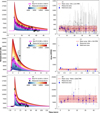 |
Fig. 4 Measured temperature evolution (left), and the evolution of the flare areas (right) for the Flares 4 (top panels), 7 (middle panels), and 8 (bottom panels). In the left panels, the black dots represent the temperature evolution determined from the multi-color observations. The color gradient area depicts the blackbody temperature evolution throughout the event for various peak temperatures of the flares. The magenta line and the shaded interval indicate the best fit and its associated uncertainty range. In the right panels, the gray dots show the flare area evolution over the entire event, with the red line representing the mean area and the shaded red interval indicating its uncertainty. Blue points with error bars show the rebinned area measurements throughout the event. The values on abscissa show time in minutes from the peak of the flare. The number in the upper part of each panel represents the number of the flare in this paper (Table 3). |
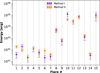 |
Fig. 5 Comparison of the flare energies estimated using Method I (violet points), and Method II (orange points). |
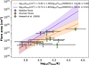 |
Fig. 6 Relationship between flare area and flare peak temperature Tflare. Flares observed at the Białków Observatory are shown in blue, while data from Howard et al. (2020) are represented in green. The flare from the Shumen Observatory is marked in red (Flare 7). The size of the point indicates the radius of the star on which the flare occurred. The purple and the orange curves, along with their shaded regions, illustrate the power-law fit to our observational data and our observational data combined with the data from Howard et al. (2020) respectively. |
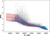 |
Fig. 7 Relation between stellar radius and effective temperature for the 16 000 most active main-sequence stars from Pietras et al. (2022) (blue dots). The red line presents the fit described by Eqs. (10)–(13), the red interval represents the fit error and the orange star corresponds to the parameters of the Sun. The gray points represent possible falsely detected main-sequence stars in the MAST catalog (2000 stars). |
4.3 Semiempirical peak temperatures of flares
Using our semiempirical grid, we calculated the peak blackbody temperatures for the sample of 42 257 flares observed on 268 most active stars from Pietras et al. (2022). Only 3% of these flares had peak temperatures below 7000 K, 22% ranged between 7000 K and 10 000 K, 42% had peak temperatures between 10 000 K and 14 000 K, 28% ranged from 14 000 K to 20 000 K, and 5% exceeded 20 000 K. The lowest estimated peak temperature was 5700 K, observed in the flare from the M4V star YZ CMi, while the highest temperature reached over 38 000 K in the flare from the M0V star TIC293507177. During the event on YZ CMi, the detected signal from the star increased by 0.2%, whereas the signal from TIC293507177 increased by approximately 135%. More than 50% of the flares had peak blackbody temperatures of approximately 11 100 ± 2400 K. The histogram showing this distribution is presented in Fig. 10.
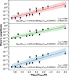 |
Fig. 8 Selected examples of relationships between estimated peak temperatures of the flares Tflare and calculated amplitudes of the flares (black dots) for three selected effective temperatures of the stars equal to 3200, 3800, and 4500 K. The red, green, and blue lines and intervals show the power-law fit with fit uncertainty. |
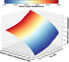 |
Fig. 9 Semiempirical relationship linking stellar effective temperature, the amplitude of its flares, and the peak temperature of the flares. The color gradient indicates the peak temperature of the flares. |
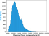 |
Fig. 10 Distribution of the peak temperatures of 42 257 flares on 268 stars, from Pietras et al. (2022), estimated using our semiempirical grid. |
5 Summary and discussion
5.1 Summary of flare observations and parameters
In this paper, we analyzed 15 stellar flares from ten different stellar objects using observations from the Białków Observatory, Shumen Observatory, TESS satellite, and flare temperature evolution from Howard et al. (2020). These stars are main-sequence stars with spectral types ranging from M5.5V to K5V (nine M-dwarfs and one K-dwarf). We were able to estimate the evolution of both the flare temperatures and flare areas during the events for the five flares observed at Białków and the two flares observed at Shumen. Additionally, we estimated the area evolution for eight flares using temperature data from Howard et al. (2020). The analyzed flares exhibited peak temperatures ranging from 5700 ± 450 K to 31 500 ± 10 050 K, with areas spanning from 50 ± 30 ppm to 7600 ± 3000 ppm.
For the analyzed events, the flare area varied in a limited range throughout the events. The relative change of the area obtained from linear fit for most of the flares did not reach level of 30% (Flares 1, 4, 8, 9, 10, 12, 13, 15). The total range of relative area changes was between 10% and 61%. In contrast, the flare temperature exhibited significant systematic variations increasing on average by factor 2.5. It should be noted that during the flare’s early phase – when the contrast ratio is sufficiently high – our estimated flare-area values are quite reliable, with relative uncertainties of only about 10%. In the late phase, however, as the contrast ratio drops, uncertainties can grow to exceed 100% of the calculated area. Consequently, the adaptive rebinning procedure described in Section 4.1 is essential for stabilizing these estimates. By applying this rebinning, we obtain mean flare-area values with relative uncertainties of 50%. The most pronounced change in flare area occurred during the impulsive phase, when the flare fully emerges before reaching a stabilized state. This phase of the evolution is hard to control with the time cadence achieved in both our observations and in Howard et al. (2020) data. In a contrast Hawley et al. (2003) or Kowalski et al. (2013) have reported significant variations in both flare area and temperature. The results for the analyzed flares may not necessarily apply to all flares. Flares 6 and 10 exhibit significant uncertainties in their peak temperature estimates, reaching up to 10 000 K. Since both the Evryscope and TESS bandpasses are located near the tail of the Planck curve, high temperatures result in very little energy being emitted within the TESS bandpass. This makes determining the temperature increasingly challenging and introduces significant uncertainties in the measured temperature values at higher temperatures for the Flare 10. In the case of Flare 6, the absence of TESS data, coupled with the flare’s relatively low amplitude compared to the noise level in the r′ band significantly affected the accuracy of the derived temperature, leading to larger errors.
5.2 Optical thickness and energy considerations
It is commonly assumed that the emission emitted by a flare in the continuum spectrum originates from a vertical narrow chromospheric condensation region (Livshits et al. 1981) and that the condensation maintains a constant kinetic temperature of approximately 10 000 K. In such a scenario, the optical continuum of superflares becomes optically thick causing the radiation to thermalize to the blackbody at chromospheric condensation kinetic temperature. However, this assumption is not always met, particularly for observed low-energy flares below a superflare threshold. This was demonstrated using the RHD simulations by Kowalski et al. (2015, 2017, 2022) who explored the temperature, densities, and the optical-thickness evolution of the chromospheric condensation in solar and stellar flares. Flares with a chromospheric condensation layer characterized by a high electron density, ne > 5 × 1014 cm−3, and peak blackbody temperatures around 10 000 K or higher, exhibit optical spectra that closely match the Planck function and the condensation is optically thick in the Paschen continuum (e.g., Kowalski et al. 2015). The bolometric energies of Flares 8, 10, 11, 12, 13, and 15 surpass the superflare energy threshold, with their peak temperatures exceeding 10 000 K. Assuming that these flares had optically thick continua, our energy estimations are well suited for these events. The bolometric energies of Flares 1, 2, 3, 4, 5, 6, 7, 9, and 14 were below the superflare energy threshold, suggesting they may not conform to the assumption of an optically thick blackbody continuum spectrum. For these flares, an alternative method that includes the emission measure as an additional free parameter alongside the chromospheric condensation temperature and flare area may be necessary to accurately fit the observed flux enhancements using a simple cloud model for isothermal condensations (Simões et al. 2024; Heinzel 2024).
5.3 Validation of temperature estimation method
The flare’s area and temperature changes can be estimated using the peak blackbody temperature during the event. To make this temperature estimation possible, we developed a semiempirical grid based on the 14 out of 15 flares analyzed in this study. This grid establishes relationships among peak flare amplitude, peak blackbody flare temperature, and effective temperature of the star. The grid is designed for use with main-sequence stars that have temperatures ranging from 2700 K to 4600 K, enabling the estimation of the peak flare temperature and its associated uncertainty. The grid provides a reasonably accurate approximation, with differences between the grid-estimated and observed values consistently falling within a 30% margin. We tested our grid using three different spectral models: ATLAS9 (Castelli & Kurucz 2004a), PHOENIX, and TURBOSPECTRUM (Gerber et al. 2023). Regardless of which spectra were used to create the grid, we obtained very similar results for the maximum flare temperatures with differences up to 5%. We evaluated our methods for estimating temperature and area by analyzing the IF3 flare on YZ CMi, as described in Kowalski et al. (2013). This analysis also served to validate our grid against results obtained from spectroscopy. During the IF3 event, as estimated by Kowalski et al. (2013), the temperature of the flaring region rose from approximately 10 000 K at the beginning of the flare to around 12 100 K at its peak, and then decayed to approximately 7000 K. Simultaneously, the flare’s area ranged between 0.2% and 1.0% of the stellar disk. Using the gri photometry included of this event (]hboxKowalski et al. 2013), we determined the temperature evolution of IF3 with the method presented in Sect. 3.1. Our estimation of the peak flare temperature was 13 000 ± 3200 K, which aligns well with the value of ∼12 100 K reported by Kowalski et al. (2013). While our estimated flare area showed minor variations, it could be approximated as a constant value of 0.70% ± 0.01% of the stellar disk, which also agrees closely with the values reported by Kowalski et al. (2013). It is important to note that we did not have TESS photometric data for this event, as TESS was launched in 2018, whereas the IF3 flare was observed in 2011. To estimate the peak temperature using our grid, we generated synthetic TESS data based on the analysis in Kowalski et al. (2013) for IF3. This synthetic data was derived from the temperature and area obtained from spectra, which we consider the most reliable source. Using Eqs. (8) and (9), along with the temperature and area evolution from Kowalski et al. (2013) and the theoretical PHOENIX spectrum for YZ CMi, we estimated the flare amplitude to reach ∼0.204 in the normalized light curve of the star in TESS bandpass. This corresponds to a temperature of 14 400 ± 2600 K, as estimated using our grid. Additionally, we repeated the same process using the temperature and area evolution derived from gri photometric estimations. In this case, the flare amplitude reached ∼ 0.271 in the normalized light curve in TESS bandpass, corresponding to a temperature of 15 300 ± 2800 K. These temperature estimates for the IF3 event were consistent within the error margins.
The key issue with the B-band is that it includes most higher-order Balmer lines rather than the Balmer jump. In addition to the line flux enhancement, as noted by Castelli & Kurucz (2004b); Kowalski et al. (2013), in this wavelength range, the Stark broadening of Balmer lines (Peterson 1969; Donati-Falchi et al. 1985) creates a pseudo-continuum, which can lead to an apparent enhancement beyond what would be expected from an extension of the optical continuum. This depends on the density of the chromospheric flares. The last resolved Balmer line is a key indicator of density, according to the Inglis-Teller formula (Inglis & Teller 1939). The corresponding results of stellar flare simulations are shown in Figures 8, 10, and 11 of Kowalski et al. (2015). To assess the impact of Balmer lines on the B-band, we evaluated their contributions by analyzing the time-evolution spectra of the IF2, IF3, and IF7 flares on YZ CMi from Kowalski et al. (2013), applying the methodology described in our paper. We estimated blackbody flare temperatures based on energy ratios in the B and pseudo-TESS bandpasses. While our pseudo-TESS bandpass does not fully cover the TESS range (extending to ∼ 9200 Å instead of ∼11 000 Å), it captures most of its sensitivity range, allowing a reasonable comparison. IF3 is classified as one of the most impulsive from Kowalski et al. (2013) sample, whereas the flares IF2 and IF7 were classified as simple, classical flares with energies below superflare threshold. These three events were selected for their relatively high signal-to-noise ratio with wavelength range reaching up to ∼ 9200 Å. Our analysis showed that the ratio of energy emitted in spectrum of the flare compared to the blackbody emission in the B-band varies between 2.5% and 7.5% throughout the IF3 flare event, and between approximately 2% and 10% throughout the IF2 and IF7 events, with the highest values occurring in the early decay phase, and lowest in the late decay phase. This leads to a possible overestimations by the value up to 10%. Given the measurement uncertainties, this effect is negligible and does not significantly impact our results. Similarly, the temperature estimations using B-band and pseudo-TESS band-passes lead to similar temperature evolution values as estimated by Kowalski et al. (2013) within the uncertainty range of up to approximately 10% of the value. The broadening of high-order Balmer lines indeed contributes to the blue continuum, but our estimates indicate that this may not lead to a substantial overestimation of the temperature when using both B-band and TESS data.
5.4 Flare energy estimates and limitations
Although our grid requires further refinement and the inclusion of additional flares, this initial version provides a valuable tool for approximating flare temperatures. In the next phase of analysis, we estimated the total energy of the IF3 event based on the temperature evolution derived from photometry, spectra, and Method II. Using Method II, we calculated a total energy of 8.3 × 1033 erg. From the temperature evolution derived from spectra, we obtained an energy of approximately 1.6 × 1033 erg, and from the temperature evolution derived from gri photometry, we calculated an energy of approximately 2.5 × 1033 erg.
The bolometric energies of the 15 analyzed flares ranged from (2.0 ± 1.3) × 1031 erg to (1.2 ± 0.5) × 1035 erg based on the observational data. The total flare energy is directly proportional to the projected flare area on the star (Eq. (7)). However, without precise details about the flare’s position on the stellar disk, the actual flare area could be significantly larger than the projected area. This discrepancy likely results in an underestimation of the flare energy. Consequently, our current energy estimates should be regarded as lower bounds. The energy values differed by less than 1% regardless of the area evolution was based on actual data or approximated as a constant mean value throughout the event. A similar outcome was observed when estimating bolometric energy using either a constant mean area or a minimally evolving area derived from interpolated values of the flare’s peak temperature and light curve.
In the case of the energy estimation method introduced by Shibayama et al. (2013), changes in temperature values can significantly affect energy estimates, although this effect is not always obvious. It arises from the anti-correlation between temperature values and the flare emission area. It should also be noted that this influence varies with the observational band used. For example, in the TESS band, when the flare peak temperature is around 10 000 K, bolometric energy estimations depend in the blackbody model as follows: E ∼ T 2. However, at 20 000 K, this dependence shifts to approximately E ∼ T 2.5. In contrast, if the flare temperature is around 5500 K, the flare energy remains largely unaffected by changes in temperature. All the above calculations were performed assuming an effective stellar temperature of 3300 K, which is the average value for spectral type M.
Our analysis of 42 257 peak blackbody flare temperatures from 268 of the most active stars in the TESS data, with temperatures lower than 4600 K, reveals that over 50% of the flares have peak temperatures around 11 100 ± 2400 K. Flares typically have a fast rise and a slower exponential decay, which means that during the majority of the flare, the temperature will be notably lower than the peak value (less than 10 000 K). Consequently, the Method II may overestimate flare energies in such cases. Flares 1 and 6 are good examples of this overestimation, as their peak temperatures are 5700 ± 450 K and 17 500 ± 10 000 K, respectively. However, temperatures above 10 000 K are observed for only 90 seconds, or 5% of the total duration for the Flare 6, and the Flare 1 does not reach 10 000 K at all. Additionally, the areas estimated using the Method II are lower for the Flare 1 by a factor of three, and higher the Flare 6 by a factor of 15. This leads to an overestimation of flare energy by 300% – 400% for both flares.
5.5 Big flare syndrome and possible statistical trends
For stellar flares, studies by Pietras et al. (2022, 2023) and others suggest that the standard solar flare model is applicable beyond the Sun. Similar physical processes likely take place on other stars, though on a much larger scale, implying that the BFS phenomenon may also be present. The “Big Flare Syndrome” (BFS) describes a statistical trend in which all energetic flare phenomena, including soft and hard X-ray emissions, become more intense in larger flares, regardless of specific physical mechanisms Kahler (1982). This pattern, well-documented in solar flares, is expected to occur on other stars as well. The relationship between white-light, hard, and soft X-ray emissions can be attributed to non-thermal electrons: those accelerated in the corona during magnetic reconnection deposit energy in the chromosphere through bremsstrahlung, producing hard X-ray emission at the footpoints. Simultaneously, these electrons heat the chromosphere, leading to evaporation that fills magnetic loops and generates soft X-ray emission. The peak temperatures of the observed flares, when compared to their mean areas throughout the event, show a positive correlation (with a probability of p = 0.98). This correlation suggests that, in stellar flares, higher flare energies correspond to larger flare areas observed in white light and to higher peak temperatures, much like in the solar case. Thus, Fig. 6 likely illustrates this BFS relationship, as slightly larger flare regions appear to be associated with higher peak temperatures. However, due to the limited sample size, further observations are necessary to explore this scenario in greater detail. Based on the estimated flare areas, we conducted statistical tests to examine whether the analyzed events form two distinct groups. Using Student’s t-test, we compared the peak blackbody temperatures of the flares, obtaining a p value of approximately 0.09 and a t-statistic of about 2.15. While this does not provide strong evidence for a statistically significant difference at the 5% level, it suggests a potential trend where larger flares may have higher peak temperatures. For flare areas, the Mann-Whitney U test yielded a p value of approximately 0.001, indicating a statistically significant difference between the two groups. We also investigated whether flare sizes correlate with stellar spectral types and found that larger flares predominantly occurred on earlier-type stars (M4V to K5V), while smaller flares were mostly observed on later-type stars (M5.5V to M2V). Further investigation is needed to explore these trends more thoroughly.
6 Conclusions
In summary, our analysis leads to two key conclusions:
We examined the temperature evolution of seven newly observed flares. Flare areas of these flares, and additional flares from Howard et al. (2020), remained constant within the 30% (on the average) throughout their duration and can be treated as fixed. The issue of how big is the population of flares that do exhibit significant changes in their areas needs further investigation;
We developed a semiempirical grid for estimating flare temperatures in main-sequence stars, applicable for stellar effective temperatures up to 4600 K, using TESS data. This tool has the potential to enhance flare energy estimation for missions such as TESS and ESA’s PLATO. Future work should prioritize obtaining additional high-quality observations of flares on F and G stars. Such data are essential to validate whether the flare characteristics observed in M and K dwarfs are similarly applicable to these higher-temperature stars. In this context, our established relationships between the effective temperature and the radius of main-sequence stars could prove instrumental in calibrating the grid for these additional flaring stars, ultimately enhancing the robustness of our methods.
The findings underscore the importance of improving flare observation statistics through multicolor photometry and spectroscopy. Achieving this requires coordinated observation campaigns utilizing both ground-based and satellite platforms. Looking ahead, designing a future space mission with capabilities to observe in two or more photometric bands, similar to TESS or PLATO, would be a significant step forward.
Acknowledgements
This work was partially supported by the program “Excellence Initiative – Research University” for the years 2020–2026 for the University of Wrocław, project No. BPIDUB.4610.96.2021.KG. Additional partial support was also provided by the grant of the Czech Funding Agency Nos. 22-30516K and RVO:67985815. D. Marchev acknowledges project RACIO supported by the Ministry of Education and Science of Bulgaria (Bulgarian National Roadmap for Research Infrastructure). The authors appreciate the constructive comments and suggestions from the anonymous referees, which have been very helpful in improving the manuscript. The computations were performed using resources provided by Wrocław Networking and Supercomputing Centre (https://wcss.pl), computational grant number 569. This paper includes data collected by the TESS mission. NASA’s Science Mission Directorate provides funding for the TESS mission.
References
- Angelov, T. 1996, Bull. Astron. Belgrade, 154, 13 [Google Scholar]
- Bessell, M. S. 1991, AJ, 101, 662 [Google Scholar]
- Bicz, K., Falewicz, R., Pietras, M., Siarkowski, M., & Preś, P. 2022, ApJ, 935, 102 [NASA ADS] [CrossRef] [Google Scholar]
- Bicz, K., Falewicz, R., & Pietras, M. 2024, A&A, 682, A176 [NASA ADS] [CrossRef] [EDP Sciences] [Google Scholar]
- Boyajian, T. S., von Braun, K., van Belle, G., et al. 2017, ApJ, 845, 178 [Google Scholar]
- Cassisi, S., & Salaris, M. 2019, A&A, 626, A32 [NASA ADS] [CrossRef] [EDP Sciences] [Google Scholar]
- Castelli, F., & Kurucz, R. L. 2004a, New Grids of ATLAS9 Model Atmospheres [Google Scholar]
- Castelli, F., & Kurucz, R. L. 2004b, New Grids of ATLAS9 Model Atmospheres [Google Scholar]
- Cliver, E. W., & Dietrich, W. F. 2013, J. Space Weather Space Climate, 3, A31 [Google Scholar]
- Davenport, J. R. A., Hawley, S. L., Hebb, L., et al. 2014, ApJ, 797, 122 [Google Scholar]
- Davenport, J. R. A., Hebb, L., & Hawley, S. L. 2015, ApJ, 806, 212 [Google Scholar]
- Davenport, J. R. A., Mendoza, G. T., & Hawley, S. L. 2020, AJ, 160, 36 [NASA ADS] [CrossRef] [Google Scholar]
- Donati-Falchi, A., Falciani, R., & Smaldone, L. A. 1985, A&A, 152, 165 [NASA ADS] [Google Scholar]
- Dudík, J., Polito, V., Janvier, M., et al. 2016, ApJ, 823, 41 [Google Scholar]
- Durán, J. S. C., & Kleint, L. 2020, ApJ, 904, 96 [CrossRef] [Google Scholar]
- Falewicz, R. 2014, ApJ, 789, 71 [NASA ADS] [CrossRef] [Google Scholar]
- Fisher, G. H. 1989, ApJ, 346, 1019 [Google Scholar]
- Fisher, G. H., Canfield, R. C., & McClymont, A. N. 1985a, ApJ, 289, 414 [NASA ADS] [CrossRef] [Google Scholar]
- Fisher, G. H., Canfield, R. C., & McClymont, A. N. 1985b, ApJ, 289, 425 [Google Scholar]
- Froning, C. S., Kowalski, A., France, K., et al. 2019, ApJ, 871, L26 [NASA ADS] [CrossRef] [Google Scholar]
- Gaia Collaboration (Brown, A. G. A., et al.) 2021, A&A, 649, A1 [NASA ADS] [CrossRef] [EDP Sciences] [Google Scholar]
- Gerber, J. M., Magg, Ekaterina, Plez, Bertrand, et al. 2023, A&A, 669, A43 [NASA ADS] [CrossRef] [EDP Sciences] [Google Scholar]
- Gershberg, R. E., & Shakhovskaya, N. I. 1972, Soviet Ast., 15, 737 [Google Scholar]
- Gryciuk, M., Siarkowski, M., Sylwester, J., et al. 2017, Sol. Phys., 292, 77 [NASA ADS] [CrossRef] [Google Scholar]
- Günther, M. N., Zhan, Z., Seager, S., et al. 2020, AJ, 159, 60 [Google Scholar]
- Hawley, S. L., & Fisher, G. H. 1992, ApJS, 78, 565 [NASA ADS] [CrossRef] [Google Scholar]
- Hawley, S. L., Fisher, G. H., Simon, T., et al. 1995, ApJ, 453, 464 [NASA ADS] [CrossRef] [Google Scholar]
- Hawley, S. L., Allred, J. C., Johns-Krull, C. M., et al. 2003, ApJ, 597, 535 [Google Scholar]
- Hawley, S. L., Walkowicz, L. M., Allred, J. C., & Valenti, J. A. 2007, PASP, 119, 67 [Google Scholar]
- Heinzel, P. 2024, MNRAS, 532, L56 [Google Scholar]
- Henry, T. J., Walkowicz, L. M., Barto, T. C., & Golimowski, D. A. 2002, AJ, 123, 2002 [NASA ADS] [CrossRef] [Google Scholar]
- Howard, W. S., Corbett, H., Law, N. M., et al. 2020, ApJ, 902, 115 [Google Scholar]
- Husser, T.-O., Wende-von Berg, S., Dreizler, S., et al. 2013, A&A, 553, A6 [NASA ADS] [CrossRef] [EDP Sciences] [Google Scholar]
- Ikuta, K., Namekata, K., Notsu, Y., et al. 2023, ApJ, 948, 64 [Google Scholar]
- Ilin, E., Poppenhaeger, K., Schmidt, S. J., et al. 2021, MNRAS, 507, 1723 [CrossRef] [Google Scholar]
- Inglis, D. R., & Teller, E. 1939, ApJ, 90, 439 [NASA ADS] [CrossRef] [Google Scholar]
- Jeffers, S. V., Barnes, J. R., Schöfer, P., et al. 2022, A&A, 663, A27 [NASA ADS] [CrossRef] [EDP Sciences] [Google Scholar]
- Joy, A. H., & Abt, H. A. 1974, ApJS, 28, 1 [Google Scholar]
- Kahler, S. W. 1982, J. Geophys. Res., 87, 3439 [NASA ADS] [CrossRef] [Google Scholar]
- Kjurkchieva, D., Marchev, D., Borisov, B., et al. 2020, Bulg. Astron. J., 32, 113 [Google Scholar]
- Kowalski, A. F. 2024, Liv. Rev. Sol. Phys., 21, 1 [NASA ADS] [CrossRef] [Google Scholar]
- Kowalski, A. F., & Allred, J. C. 2018, ApJ, 852, 61 [Google Scholar]
- Kowalski, A. F., Hawley, S. L., Wisniewski, J. P., et al. 2013, ApJS, 207, 15 [NASA ADS] [CrossRef] [Google Scholar]
- Kowalski, A. F., Hawley, S. L., Wisniewski, J. P., et al. 2013, VizieR On-line Data Catalog: J/ApJS/207/15 [Google Scholar]
- Kowalski, A. F., Hawley, S. L., Carlsson, M., et al. 2015, Sol. Phys., 290, 3487 [NASA ADS] [CrossRef] [Google Scholar]
- Kowalski, A. F., Allred, J. C., Uitenbroek, H., et al. 2017, ApJ, 837, 125 [Google Scholar]
- Kowalski, A. F., Allred, J. C., Carlsson, M., et al. 2022, ApJ, 928, 190 [NASA ADS] [CrossRef] [Google Scholar]
- Kunkel, W. E. 1975, in Variable Stars and Stellar Evolution, eds. V. E. Sherwood & L. Plaut, AU Symposium, 67, 15 [Google Scholar]
- Law, N. M., Fors, O., Ratzloff, J., et al. 2016, in Ground-based and Airborne Telescopes VI, 9906, eds. H. J. Hall, R. Gilmozzi, & H. K. Marshall, International Society for Optics and Photonics (SPIE), 99061M [Google Scholar]
- Lépine, S., Hilton, E. J., Mann, A. W., et al. 2013, AJ, 145, 102 [Google Scholar]
- Livshits, M. A., Badalyan, O. G., Kosovichev, A. G., & Katsova, M. M. 1981, Sol. Phys., 73, 269 [Google Scholar]
- Mochnacki, S. W., & Zirin, H. 1980, ApJ, 239, L27 [NASA ADS] [CrossRef] [Google Scholar]
- Morin, J., Donati, J.-F., Forveille, T., et al. 2008a, MNRAS, 384, 77 [CrossRef] [Google Scholar]
- Morin, J., Donati, J. F., Petit, P., et al. 2008b, MNRAS, 390, 567 [Google Scholar]
- Namekata, K., Sakaue, T., Watanabe, K., et al. 2017, ApJ, 851, 91 [Google Scholar]
- Notsu, Y., Shibayama, T., Maehara, H., et al. 2013, ApJ, 771, 127 [NASA ADS] [CrossRef] [Google Scholar]
- Paudel, R. R., Barclay, T., Schlieder, J. E., et al. 2021, ApJ, 922, 31 [NASA ADS] [CrossRef] [Google Scholar]
- Pecaut, M. J., & Mamajek, E. E. 2013, ApJS, 208, 9 [Google Scholar]
- Peterson, D. M. 1969, SAO Spec. Rep., 293 [Google Scholar]
- Pietras, M., Falewicz, R., Siarkowski, M., Bicz, K., & Preś, P. 2022, ApJ, 935, 143 [NASA ADS] [CrossRef] [Google Scholar]
- Pietras, M., Falewicz, R., Siarkowski, M., et al. 2023, ApJ, 954, 19 [NASA ADS] [CrossRef] [Google Scholar]
- Preś, P., Falewicz, R., & Jakimiec, J. 2005, Adv. Space Res., 35, 1739 [Google Scholar]
- Ratzloff, J. K., Law, N. M., Fors, O., et al. 2019, PASP, 131, 075001 [Google Scholar]
- Ricker, G. R., Winn, J. N., Vanderspek, R., et al. 2014, Space Telescopes and Instrumentation 2014: Optical, Infrared, and Millimeter Wave, 9143, 914320 [Google Scholar]
- Riedel, A. R., Alam, M. K., Rice, E. L., Cruz, K. L., & Henry, T. J. 2017, ApJ, 840, 87 [NASA ADS] [CrossRef] [Google Scholar]
- Robinson, R. D., Wheatley, J. M., Welsh, B. Y., et al. 2005, ApJ, 633, 447 [Google Scholar]
- Shibata, K. 1999, Ap&SS, 264, 129 [Google Scholar]
- Shibata, K., & Yokoyama, T. 2002, ApJ, 577, 422 [CrossRef] [Google Scholar]
- Shibayama, T., Maehara, H., Notsu, S., et al. 2013, ApJS, 209, 5 [Google Scholar]
- Simões, P. J. A., Araújo, A., Válio, A., & Fletcher, L. 2024, MNRAS, 528, 2562 [CrossRef] [Google Scholar]
- Torres, C. A. O., Quast, G. R., da Silva, L., et al. 2006, A&A, 460, 695 [NASA ADS] [CrossRef] [EDP Sciences] [Google Scholar]
- Upendran, V., Tripathi, D., Mithun, N. P. S., Vadawale, S., & Bhardwaj, A. 2022, ApJ, 940, L38 [Google Scholar]
- Yang, B., Yang, J., Bi, Y., Hong, J., & Xu, Z. 2021, ApJ, 921, L33 [NASA ADS] [CrossRef] [Google Scholar]
- Zhilyaev, B. E., Romanyuk, Y. O., Svyatogorov, O. A., et al. 2007, A&A, 465, 235 [NASA ADS] [CrossRef] [EDP Sciences] [Google Scholar]
Barbara A. Mikulski Archive for Space Telescopes.
Parts per million of a stellar disk.
All Tables
Information about the flares from Howard et al. (2020) used in the present paper.
Peak temperatures, mean areas, and F-test results for constancy of flare area over time.
All Figures
|
Fig. 1 Normalized light curves of five flares of EV Lac in three different passbands. The blue, green, and red curves represent the B-band, V-band made in Białków Observatory, and the 20 s TESS observations, respectively. The panels are labelled with the flare number (Table 1). |
| In the text | |
|
Fig. 2 Normalized light curve of the Flare 6 of V374 Peg in three band-passes g′, r′, and the i′ (labeled). Observations were made in Shumen Observatory. |
| In the text | |
|
Fig. 3 Normalized light curve of the Flare 7 of GJ 1243, observed in two bandpasses, g′ and r′ (labeled), at Shumen Observatory, along with the 20 s normalized light curve from TESS (labeled). |
| In the text | |
|
Fig. 4 Measured temperature evolution (left), and the evolution of the flare areas (right) for the Flares 4 (top panels), 7 (middle panels), and 8 (bottom panels). In the left panels, the black dots represent the temperature evolution determined from the multi-color observations. The color gradient area depicts the blackbody temperature evolution throughout the event for various peak temperatures of the flares. The magenta line and the shaded interval indicate the best fit and its associated uncertainty range. In the right panels, the gray dots show the flare area evolution over the entire event, with the red line representing the mean area and the shaded red interval indicating its uncertainty. Blue points with error bars show the rebinned area measurements throughout the event. The values on abscissa show time in minutes from the peak of the flare. The number in the upper part of each panel represents the number of the flare in this paper (Table 3). |
| In the text | |
|
Fig. 5 Comparison of the flare energies estimated using Method I (violet points), and Method II (orange points). |
| In the text | |
|
Fig. 6 Relationship between flare area and flare peak temperature Tflare. Flares observed at the Białków Observatory are shown in blue, while data from Howard et al. (2020) are represented in green. The flare from the Shumen Observatory is marked in red (Flare 7). The size of the point indicates the radius of the star on which the flare occurred. The purple and the orange curves, along with their shaded regions, illustrate the power-law fit to our observational data and our observational data combined with the data from Howard et al. (2020) respectively. |
| In the text | |
|
Fig. 7 Relation between stellar radius and effective temperature for the 16 000 most active main-sequence stars from Pietras et al. (2022) (blue dots). The red line presents the fit described by Eqs. (10)–(13), the red interval represents the fit error and the orange star corresponds to the parameters of the Sun. The gray points represent possible falsely detected main-sequence stars in the MAST catalog (2000 stars). |
| In the text | |
|
Fig. 8 Selected examples of relationships between estimated peak temperatures of the flares Tflare and calculated amplitudes of the flares (black dots) for three selected effective temperatures of the stars equal to 3200, 3800, and 4500 K. The red, green, and blue lines and intervals show the power-law fit with fit uncertainty. |
| In the text | |
|
Fig. 9 Semiempirical relationship linking stellar effective temperature, the amplitude of its flares, and the peak temperature of the flares. The color gradient indicates the peak temperature of the flares. |
| In the text | |
|
Fig. 10 Distribution of the peak temperatures of 42 257 flares on 268 stars, from Pietras et al. (2022), estimated using our semiempirical grid. |
| In the text | |
Current usage metrics show cumulative count of Article Views (full-text article views including HTML views, PDF and ePub downloads, according to the available data) and Abstracts Views on Vision4Press platform.
Data correspond to usage on the plateform after 2015. The current usage metrics is available 48-96 hours after online publication and is updated daily on week days.
Initial download of the metrics may take a while.