| Issue |
A&A
Volume 668, December 2022
|
|
|---|---|---|
| Article Number | A115 | |
| Number of page(s) | 20 | |
| Section | Stellar structure and evolution | |
| DOI | https://doi.org/10.1051/0004-6361/202243732 | |
| Published online | 09 December 2022 | |
Characterising the AGB bump and its potential to constrain mixing processes in stellar interiors
1
LESIA, Observatoire de Paris, PSL Research University, CNRS, Université Pierre et Marie Curie, Université Paris Diderot, 92195 Meudon, France
e-mail: This email address is being protected from spambots. You need JavaScript enabled to view it.
2
Univ. Rennes, CNRS, IPR (Institut de Physique de Rennes), UMR 6251, 35000 Rennes, France
3
Instituto de Astrofísica e Ciências do Espaço, Universidade do Porto, CAUP, Rua das Estrelas, 4150-762 Porto, Portugal
4
Max Planck Institute for Solar System Research, Justus-von-Liebig-Weg 3, 37077 Göttingen, Germany
Received:
7
April
2022
Accepted:
27
June
2022
Abstract
Context. In the 1990s, theoretical studies motivated the use of the asymptotic giant branch bump (AGBb) as a standard candle given the weak dependence between its luminosity and stellar metallicity. Because of the small size of observed asymptotic giant branch (AGB) samples, detecting the AGBb is not an easy task. However, this has now been made possible thanks to the wealth of data collected by the CoRoT, Kepler, and TESS space-borne missions.
Aims. It is well-known that the AGB bump provides valuable information on the internal structure of low-mass stars, particularly on mixing processes such as core overshooting during the core He-burning phase. Here, we investigate the dependence of the AGBb position on stellar parameters such as the stellar mass and metallicity based on the calibration of stellar models to observations.
Methods. In this context, we analysed ∼4000 evolved giants observed by Kepler and TESS, including red giant branch (RGB) stars and AGB stars, for which asteroseismic and spectrometric data are available. By using statistical mixture models, we detected the AGBb both in frequency at maximum oscillation power, νmax, and in effective temperature, Teff. Then, we used the Modules for Experiments in Stellar Astrophysics (MESA) stellar evolution code to model AGB stars and match the AGBb occurrence with observations.
Results. From the observations, we were able to derive the AGBb location in 15 bins of mass and metallicity. We noted that the higher the mass, the later the AGBb occurs in the evolutionary track, which agrees with theoretical works. Moreover, we found a slight increase in the luminosity at the AGBb when the metallicity increases. By fitting those observations with stellar models, we noticed that low-mass stars (M ≤ 1.0 M⊙) require a small core overshooting region during the core He-burning phase. This core overshooting extent increases toward high mass; however, above M ≥ 1.5 M⊙, we found that the AGBb location cannot be reproduced with a realistic He-core overshooting alone. Thus, additional mixing processes have to be invoked instead.
Conclusions. The observed dependence on metallicity complicates the application of the AGBb as a standard candle. Moreover, different mixing processes may occur according to stellar mass. At low mass (M ≤ 1.5 M⊙), the AGBb location can be used to constrain the He-core overshooting. At high mass (M ≥ 1.5 M⊙), an additional mixing induced, for instance, by rotation is needed to reproduce what is seen in observations.
Key words: asteroseismology / stars: oscillations / stars: interiors / stars: evolution / stars: late-type / stars: AGB and post-AGB
© The Authors 2022
 Open Access article, published by EDP Sciences, under the terms of the Creative Commons Attribution License (https://creativecommons.org/licenses/by/4.0), which permits unrestricted use, distribution, and reproduction in any medium, provided the original work is properly cited.
This article is published in open access under the Subscribe-to-Open model. This email address is being protected from spambots. You need JavaScript enabled to view it. to support open access publication.
1. Introduction
The asymptotic giant branch (AGB) is a key stage of stellar evolution that can be used to constrain both the stellar structure and environment. On the one hand, observations of circumstellar CO line emission and stellar light scattered by dust in circumstellar envelopes allow us to estimate the mass-loss rate on the AGB, which is crucial in understanding the final stages of stellar evolution and the metal enrichment in the interstellar medium, and, hence, the chemical enrichment of galaxies (e.g. Knapp et al. 1998; Mauron & Huggins 2006; Ramstedt et al. 2008; McDonald et al. 2018; McDonald & Trabucchi 2019). On the other hand, the AGB provides valuable constraints for stellar interiors with the help of stellar models (Bossini et al. 2015). Current stellar models suffer from systematic uncertainties due to our limited understanding of physical processes in stellar interiors. In particular, constraining mixing processes in advanced burning stages is demanding because it requires the implementation of helium semiconvection to take into account the additional helium captured by the growing He-core (e.g. Castellani et al. 1971a; Robertson & Faulkner 1972; Sweigart & Gross 1973; Salaris & Cassisi 2017). Then, the use of observational constraints linked to stellar interiors is crucial in testing the reliability of stellar models. With this in mind, several studies aimed at constraining stellar parameters of red giants with asteroseismic observables (di Mauro et al. 2011; Baudin et al. 2012; Lagarde et al. 2015). Using the global seismic parameters, namely, the large frequency separation, Δν, and the frequency of the maximum oscillation power, νmax, these authors were able to infer the mass and radius of red giants and reduce their uncertainties by a factor of more than 3, compared with those based on spectroscopic constraints only. On top of these asteroseismic observables, the use of both the mode inertias and coupling factor between the g- and p-mode cavities in red giants provides unique constraints on mode trapping, hence, on the innermost stellar structure (Benomar et al. 2014; Pinçon et al. 2020). However, all the studies mentioned above focus on the early stages of red giants, so additional work needs to be done to constrain stellar structure during the helium-burning stages.
One of the key events happening in the helium-burning phase that still needs to be constrained is the AGBb. This has now been made possible with the recent seismic constraints obtained for high-luminosity RGB and AGB stars with Δν ≤ 4.0 μHz (Dréau et al. 2021). The AGBb is manifested through a luminosity drop as a star evolves on the AGB and is associated with the ignition of the He-burning shell source. The AGBb is then characterised by a local excess of stars in the luminosity distribution of stellar populations. While the AGBb was first predicted by stellar evolutionary models (Caputo et al. 1978), it has since been identified in the colour-magnitude diagram of a few Galactic globular clusters (Ferraro 1992). Bossini et al. (2015) showed that the AGBb can be used to constrain the core mixing scheme during the core He-burning phase. They could reproduce both the seismic constraints and the AGBb luminosity of observed Kepler red clump stars by considering core overshooting of the mixed He core with a moderate value of core overshooting (αov, He = 0.5, where αov, He is the ratio of the overshooting length to the pressure scale height). Using the AGBb luminosity as a stellar model constraint allows us to reduce the systematic uncertainties on the mixing processes beyond the boundary of the convective envelope, which are essential to predict stellar lifetime in the core He-burning phase (e.g. Castellani et al. 1971b; Chiosi 2007).
A characterisation of the luminosity bump on the RGB based on seismic data has already been achieved (Khan et al. 2018). By combining Kepler and APOGEE data on thousands of red giants, these authors brought to light the fact that the location of the red giant branch bump (RGBb) is sensitive to the stellar mass and metallicity. Moreover, they showed that significant overshooting from the base of the convective envelope during the main sequence must be behind the reproduction of the location of the RGBb, with an efficiency that increases with decreasing metallicity. A similar description of mixing beyond the convective envelope during He-burning phases would help to predict the third dredge-up efficiency on the thermally pulsing AGB (TP-AGB) phase (Herwig et al. 2000; Marigo & Girardi 2007; Wagstaff et al. 2020). Moreover, a precise characterisation of the AGBb would confirm or disprove the potential of the AGBb to be a suitable candidate for standard candles (Pulone 1992; Ferraro 1992).
This study is aimed at detecting and characterising the AGBb. First, we investigated its dependence with the stellar mass and metallicity by using Kepler and TESS asteroseismic targets. Then, we used the AGBb as a calibrator for mixing processes, particularly for core overshooting during the He-burning phase. The article is organised as follows. The data set is described in Sect. 2. In Sect. 3, we define the macrophysics and microphysics implemented to model stellar evolution up to the AGB phase. The methods we used to locate and characterise the AGBb in models and observations are presented in Sect. 4. The results are analysed in Sect. 5, illustrating the need to take He-core overshooting into account in stellar models to reproduce the observed location of the AGBb. We discuss our results and explore the impact of other parameters on the AGBb location in Sect. 6. Finally, we present our conclusions in Sect. 7.
2. Data set
In order to detect the AGBb, we selected evolved stars that have been observed by the Kepler and TESS telescopes, including RGB and AGB stars. In order to reject red clump stars from the sample, we only kept stars with νmax ≤ 22 μHz (or, equivalently, Δν ≲ 2.7 μHz) because no AGBb is expected to occur above this limit (Dréau et al. 2021, their Fig. 9). It has been shown that at low νmax ≤ 10 μHz (or equivalently Δν ≲ 1.5 μHz), it is difficult to safely distinguish AGB stars from RGB ones (Kallinger et al. 2012; Mosser et al. 2019). On the other hand, the local excess associated to the AGBb is well visible on top of the background composed of RGB and He-burning stars (Bossini et al. 2015). Therefore, since our aim here is to work on the basis of a sample containing as many AGB stars as possible, we decided not to reject any (suspected) RGB star from the initial sample. Considering more stars, even unclassified ones, allowed us to include more AGB stars in our sample. The evolved Kepler targets around this evolutionary stage have been the subject of an exhaustive seismic analysis (Mosser et al. 2013, 2014, 2019; Stello et al. 2014; Yu et al. 2020, 2021; Dréau et al. 2021), providing estimates of νmax. Then, we used the νmax estimates from Mosser et al. (2014, 2019), while we selected their mass M from the APOKASC catalogue (Pinsonneault et al. 2014, 2018). The later is a survey of Kepler targets complemented by spectroscopic data. The effective temperatures Teff and stellar metallicities are taken from the catalogues of APOGEE DR17 (Abdurro’uf et al. 2022), GALAH DR3 (Buder et al. 2021), and RAVE DR6 (Steinmetz et al. 2020). We took the stellar masses derived from the semi-empirical asteroseismic scaling relation presented in Kjeldsen & Bedding (1995), and corrected by a factor that is adjusted star by star, when available1 (Pinsonneault et al. 2018). When stellar masses are not available, which concerns about 10% of our Kepler targets, we estimated them with the semi-empirical relation without any correction factor. As for the TESS targets, they have been studied in Mackereth et al. (2021). We picked νmax as the mean value between three pipelines (Mosser & Appourchaux 2009; Mathur et al. 2010; Elsworth et al. 2020). We extracted the mass, M, effective temperature, Teff, and metallicity, [Fe/H], in the same way as for the Kepler targets. To sum up, roughly 70% of the spectroscopic estimates are from the APOGEE DR17 catalogue, 2% are from GALAH DR3, and 28% are from RAVE DR6. The typical uncertainties on the global parameters obtained in this way are: σM = 12%, σ[Fe/H] = 0.06 dex, σTeff = 64 K, σνmax = 9%. Our final sample is composed of 4099 stars, including RGB and AGB stars, as well as stars leaving the clump phase. Some of them are shown in given bins of mass and metallicity in Fig. 1.
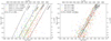 |
Fig. 1. Seismic HR diagram of our sample of stars in the bin of mass, M ∈ [0.9, 1.2] M⊙ (left) and in the bin of metallicity, [Fe/H] ∈ [ − 0.25, 0.0] dex (right). In both panels, stars with different metallicities (left) and masses (right) are represented with different colours. On top of those observations, stellar evolutionary tracks along the AGB are represented with black lines at different metallicities at 1 M⊙ (left) and masses at [Fe/H] = −0.25 dex (right). |
3. Stellar models
Evolutionary tracks and stellar models are derived with release 12778 of the stellar evolution code known as Modules for Experiments in Stellar Astrophysics (MESA, Paxton et al. 2011, 2013, 2015, 2018, 2019). We computed a grid of stellar models with initial masses of M = [0.8, 0.9, 1.0, 1.1, 1.2, 1.5, 1.75, 2.0, 2.5] M⊙ and initial metallicities of [Fe/H] = [ − 1.0, −0.5, −0.25, 0.0, 0.25] dex. The initial fractional abundance of metals in mass was set following the solar chemical composition described in Asplund et al. (2009). The treatment of convection is based on the mixing-length formalism presented in Henyey et al. (1965), which takes the opacity of the convective eddies into account. The initial helium abundance Y0, the metallicity [Fe/H] and the mixing-length parameter αMLT were calibrated to reproduce the present solar luminosity, radius, and surface metal abundance. To this end, we adapted the MESA test suite case simplex_solar_calibration and took the log L, log R, and Z/X terms2 into account in the χ2 value. We performed the solar calibration without microscopic diffusion. This gave us the solar-calibrated values Y0 = 0.253, [Fe/H] = 0 (equivalently, Z0 = 0.0133), and αMLT = 1.92 at a solar age of 4.61 Gyr3. We did not assume any coupling of Y and Z through the ΔY/ΔZ helium-to-metal Galactic enrichment ratio, but, rather, we explored different values of the couple (Y, Z).
We started from the 1M_pre_ms_to_wd test suite case and customised the physical ingredients to model stellar evolution up to the AGB. To follow chemical changes and the production of nuclear energy, we used a network of 32 nuclear reactions involving 23 stable or unstable species from 1H to 24Mg. The thermonuclear reaction rates are taken from NACRE (Angulo et al. 1999) and CF88 (Caughlan & Fowler 1988), with priority for the NACRE rates when available. We took into account some updates to crucial reaction rates at evolved stages, such as 14N(p, γ)15O (Imbriani et al. 2004) and triple-α (Fynbo et al. 2005).
Opacity values are required to compute the energy transport in regularly stratified regions, namely, in radiative zones. At low temperatures (log T < 3.95), we used the opacity tables from AESOPUS (Marigo & Aringer 2009), whereas at high temperatures (log T > 4.05), we took either the OPAL1 or OPAL2 opacity tables (Iglesias & Rogers 1996). The AESOPUS and OPAL1 tables are aimed at the Asplund et al. (2009) solar mixture, while the OPAL2 tables allow us to account for the metal mixture changes due to the C and O enhancements that result from He burning. In the region around log T = 4.00 ± 0.05, we performed a blend according to the description from Paxton et al. (2011; see their Eq. (1)) between the AESOPUS and OPAL1 tables. Furthermore, in the regions with C and O enhancements where the initial metallicity Z0 is increased by an amount dZ, we used the OPAL2 opacity tables. A blend between OPAL1 and OPAL2 is made in the region where dZ ∈ [0.001, 0.01]. Finally, the resulting opacity is combined with the electron conduction opacity, as prescribed in Cassisi et al. (2007).
We considered convective core overshooting during the main sequence, following a step scheme (e.g. Maeder 1975). This means that the mixing region extends over a distance, dov, toward the surface from the boundary of convective instability in the core where the Schwarzschild condition, ∇rad > ∇ad, is fulfilled. If HP ≤ Rcc, where HP is the pressure scale height at the boundary of the convective core and Rcc is the convective core radial thickness, then we keep dov = αov, HHP; otherwise dov = αov, HRcc. We adopted the overshooting parameter of αov, H = 0.2 in the reference model. Similarly, we computed evolutionary tracks with and without convective core overshooting during the core He-burning phase following two scenarios: either the temperature gradient ∇T is kept equal to the radiative gradient ∇rad (usual overshooting scenario) or it is maintained as equal with regard to the adiabatic temperature gradient ∇ad (penetrative convection scenario) in the overshooting region (Zahn 1991). The Schwarzschild convective border is in an unstable equilibrium in the sense that a small expansion of the convective core may make ∇rad larger than ∇ad at the new border (Castellani et al. 1971b). Adding core overshooting during the core He-burning phase induces a possible local minimum and maximum in ∇rad in the extra-mixing region due to the increasing opacity that results from the transport of C and O elements in that region. Should this maximum increase above ∇ad, a separate convective instability would occur in the overshooting region in the absence of an appropriate treatment of semi convection. To address this issue, we allowed a partially mixed He-semiconvection region (Castellani et al. 1971a) between the minimum of ∇rad and the outer radiative zone following the diffusion scheme of Langer et al. (1985), with the efficiency factor αsc = 0.1. In parallel, we followed the treatment proposed by Bossini et al. (2017) to consider a stable convective border and suppress such spurious convective instabilities. This treatment consists in defining the convective border at the point, where ∇rad has reached its local minimum if the local maximum of ∇rad has increased over ∇rad in the extra-mixing region. The convective boundary is set at the point where ∇rad = ∇ad.
We also explored the effect of envelope undershooting, which induces an extra-mixing region of extent αov, envHP below the convective envelope into the radiative core. In a process that is similar to convective core overshooting, we adopted a step scheme and applied envelope undershooting from the main sequence up to the AGB, with ∇T = ∇rad in the extra-mixing region. The typical value for low-mass red giants (M ≤ 1.6 M⊙) at solar metallicity recommended by Khan et al. (2018), namely, αov, env = 0.3, is considered here.
Other transport processes arise in stellar interiors, such as thermohaline mixing and rotation-induced mixing. Thermohaline convection starts along the RGB in regions that are stable against convection (according to the Ledoux criterion) and where the molecular weight gradient becomes negative (i.e. ∇μ = dlnμ/dlnP < 0) between the H-burning shell surrounding the degenerate core and the convective envelope. This composition gradient inversion is induced by the 3He(3He, 2p)4He reactions that take place around the H-burning shell (Ulrich 1972; Eggleton et al. 2006, 2008; Charbonnel & Zahn 2007). Here, thermohaline mixing is treated in a diffusion approximation based on the work of Kippenhahn et al. (1980), where the corresponding diffusion coefficient is expressed as (Paxton et al. 2013):
 (1)
(1)
In the previous equation, K is the radiative conductivity, cP is the specific heat at constant pressure, αth is the efficiency parameter for the thermohaline mixing, and we have:
 (2)
(2)
where χT = (∂lnP/∂lnT)ρ and Xi represents the mass fraction of atoms of species, i, in the N-component plasma. The species j is eliminated in the sum so that the constraint  is fulfilled. We adopted αth = 2, which corresponds to the prescription of Kippenhahn et al. (1980) where blobs of size L diffuse while travelling over a mean free path L before dissolving. We checked that the extent of the extra mixing regions caused by thermohaline convection is in agreement with the one obtained by Cantiello & Langer (2010). In particular, we verified that the extra mixing region is large enough to connect the H-burning shell and the convective envelope during the core He-burning phase for stars with a mass below 1.5 M⊙.
We investigated the effects of rotation on the AGBb location since rotation is known to impact lifetimes, surface abundances, and evolutionary fates. Rotation is treated in 1D in the shellular approximation (e.g. Meynet & Maeder 1997). Further information can be found in Paxton et al. (2013), particularly regarding how rotation is implemented in MESA treated as a diffusive process. We took rotation into account from the zero-age main sequence (ZAMS), as is often done in stellar evolution codes (e.g. Pinsonneault et al. 1989), up to the terminal-age main sequence (TAMS). First, we implemented rotation up to the early AGB phase, but it made the evolutionary track noisy at the AGBb without modifying its position. Therein, we only maintained the rotation during the main sequence. The rotation rate gradually reaches the maximum value ΩZAMS/Ωcrit = 0.3, where Ωcrit is the surface critical angular velocity for the star to be dislocated, which is the typical rotation rate motivated by observations of B stars (Huang et al. 2010). For a 2 M⊙ star, the evolutionary track that includes the rotation rate ΩZAMS/Ωcrit = 0.3 during the main sequence is equivalent to one that includes a H-core overshooting αov, H ≈ 0.25. We checked that the evolution of the surface rotation rate so obtained along the main sequence is similar to that obtained in Ekström et al. (2012). We only studied rotating models with M ≥ 1.5 M⊙ since magnetic braking is not included in MESA, which does not allow for the reproduction of slow rotation rates for low-mass stars (Kawaler 1988).
Rotation induces both chemical and angular momentum transports through instabilities that are treated in a diffusion approximation (Endal & Sofia 1978; Pinsonneault et al. 1989; Heger et al. 2000). In our models, we included six equally weighted instabilities induced by rotation, namely: dynamical shear, Solberg-Høiland, secular shear, Goldreich-Schubert-Fricke instabilities, Eddington-Sweet circulation, and Tayler-Spruit dynamo. Then, each diffusion coefficient associated to those rotationally induced instabilities is added to the diffusion coefficient in absence of rotation. On top of this resulting diffusion coefficient, two free parameters need to be fixed in diffusion equations: the factor fc that scales the efficiency of composition mixing relatively to that of the angular momentum transport and the factor fμ that encodes the sensitivity of rotational mixing to the mean molecular weight gradient. Typical values from Heger et al. (2000) such as fc = 1/30 and fμ = 0.05 are adopted here.
We took a grey atmosphere with an Eddington T(τ) relation. We defined the outermost meshpoint of the models as the layer where the optical depth τ verifies τ = 2/3, which is at the limit of the photosphere. Another important parameter that impacts the fate of stars is the mass-loss rate. We used Reimers’ prescription (Reimers 1975):
 (3)
(3)
from the RGB up to the core He-burning phase, where ηR is the Reimers’ scaling factor that we take equal to ηR = 0.3 (Miglio et al. 2021). On the AGB, we use the Blöcker’s prescription (Blocker 1995):
 (4)
(4)
where ηB is the Blöcker’s scaling factor taken equal to ηB = 0.1. In both Reimers’ and Blöcker’s prescriptions, L, R, and M are expressed in solar units.
The screening factors were computed with the implementation of Chugunov et al. (2007) for weak and strong screening conditions. We kept the default coverage of the equation of state in the log ρ − log T plane (as summarised in Fig. 50 of Paxton et al. 2019).
4. Characterisation of the AGBb
4.1. Observations
Heretofore, we had found that the AGBb is manifested as a local excess of stars on top of a background composed of RGB and AGB stars. In order to infer the AGBb location in νmax and Teff, in the way that Khan et al. (2018) proceeded to characterise the RGBb, we adopted the statistical mixture model presented in Hogg et al. (2010). This approach is a statistical framework where the data set is assumed to be multimodal, that is, with several regions of high probability separated by regions of low probability. In this situation, we modelled the data with a mixture of several components, where each data point belongs to one of these components. This allowed us to use multiple models to fit our data set. We distinguished the inliers, which are stars belonging to the AGBb overdensity and the outliers, which are stars that belong to the RGB/AGB background and do not lie in the AGBb phase. The fit was performed using the Python module Emcee, which is an affine invariant Markov chain Monte Carlo (MCMC) ensemble sampler (Foreman-Mackey et al. 2013). The likelihood function is defined as:
 (5)
(5)
where fbiv describes the AGBb foreground with a bivariate normal distribution function, fbg describes the RGB-AGB background with the product of a normalised rising exponential in log νmax and a linear term with a normally distributed scatter, and Pbg is the mixture model weighting factor that gives the probability for a star to belong to the RGB-AGB background. The foreground and background probability distribution functions are:
 (6)
(6)
and
 (7)
(7)
respectively. In the previous equations, x1 = log Teff and x2 = log νmax, and μ1 and μ2 are the AGBb locations in log Teff and log νmax, respectively, σ1 and σ2 are the AGBb standard deviations in log Teff and log νmax, respectively, ρ12 is the correlation of the bivariate Gaussian, abg and bbg are the linear coefficients, σbg is the standard deviation of the normal distribution of the linear term, cbg and Aexp are the coefficient and the normalisation factor of the exponential term, respectively.
Given the small amplitude of the AGBb overdensity in log νmax (see Fig. 2), σ2 failed to converge when we used the fitting method described above. Consequently, we estimated σ2 separately by fitting the AGBb overdensity with a normal distribution function in the 1D histogram of log νmax. We took this estimate and kept it fixed during the MCMC process. Then, the posterior probability distributions of our set of 9 free parameters, which are μ1, μ2, σ1, ρ12, abg, bbg, σbg, cbg, and Pbg, were visualised with the Python module Corner (Foreman-Mackey 2016). First, the guess values of the bivariate Gaussian and the exponential term were extracted from the 1D histograms in log νmax and log Teff and those of the linear term were obtained from the 2D histogram, as seen in Fig. 2. Then, the parameters were left free to vary according to a uniform prior probability distribution.
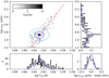 |
Fig. 2. Probability distribution functions of our data set in the log Teff; log νmax plane, in the bins M ∈ [0.9, 1.2] M⊙ and [Fe/H] ∈ [ − 0.25, 0.0] dex. Upper left panel: 2D histogram where the AGBb is located by a blue diamond. Dark blue and light blue ellipses correspond to the 1σ and 2σ regions of the bivariate Gaussian, respectively. The red dashed line reproduces the linear term belonging to the RGB/AGB background. Upper right panel: normalised 1D histogram in log νmax is shown in black. The ordinate axis is the same as in the upper left panel. The blue line corresponds to the probability distribution function made of the Gaussian associated to the overdensity in log νmax, multiplied by the rising exponential in log νmax. Lower left panel: same label as in the upper right panel but in terms of log Teff. The abscissa axis is the same as in the upper left panel. The blue line shows the Gaussian associated to the overdensity in log Teff. Lower right panel: difference between log νmax and abglog Teff + bbg. The blue line illustrates the normal distribution around the linear term. |
We performed this fitting method in the log Teff − log νmax plane, in restricted bins of mass and metallicity, which are M ∈ [0.6, 0.9], [0.9, 1.2], [1.2, 1.5], [1.5, 2.5]M⊙ and [Fe/H] ∈ [ − 1.0, −0.5], [ − 0.5, −0.25], [ − 0.25, 0.0], [0.0, 0.25] dex. The bins are wider at high mass and low metallicity to include enough stars and hence ensure the free parameters to converge. The number of stars per bin is shown in Table 1. We show in Fig. 2 the results for the bin M ∈ [0.9, 1.2] M⊙ and [Fe/H] ∈ [ − 0.25, 0.0] dex.
Number of stars per mass and metallicity bins.
4.2. Models
To extract the probability for a star to lie in a given bin of νmax and Teff along its evolutionary track, we computed the inverse of the evolution speeds, dτ/dνmax and dτ/dTeff, where τ is the stellar age. Then, we integrated dτ/dνmax and dτ/dTeff over νmax and Teff, respectively. This gives us the fractional time that is spent in a given bin of νmax and Teff, respectively. We used this fractional time as a proxy of the probability distribution for a star to lie in a given bin of νmax and Teff. The procedure was repeated for each pair of mass and metallicity in our grid of stellar models (presented in Sect. 3). We summed the probability distributions of all pairs of mass and metallicity lying in the considered bin of mass and metallicity and we normalised the resulting probability distribution. Because the grid of stellar models is discontinuous compared to observations and the probability distributions are narrow at the turning-backs of the AGBb (i.e. where the quantities of dτ/dνmax and dτ/dTeff change sign), we convolved the resulting probability distribution by a normal one. Eventually, the maximum of the convolved probability distribution was interpreted as the AGBb location.
With the aim to investigate the potential of the AGBb to constrain physical processes in stellar interiors, we attempted to make the observed AGBb location match the expected AGBb one as well as possible by comparing the 1D histograms of log νmax and log Teff from observations with the corresponding probability distributions derived from stellar models. To this end, we defined a reference model and varied the stellar parameters to explore their impact on the expected AGBb location in log νmax and log Teff. The results are presented in the following section.
5. Results
We applied the procedure described in Sect. 4 both to the data set and the stellar models and examined the AGBb location for all the bins of mass and metallicity previously introduced. The results are presented in Figs. 3−7 and Tables A.1−A.4.
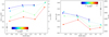 |
Fig. 3. Location of the AGBb in log νmax (left) and in log Teff (right) from observations, as a function of the metallicity, [Fe/H]. The AGBb occurrence is marked by dots and the stellar mass is colour-coded. AGBb locations obtained in the same bin of mass, M ∈ [0.6, 0.9], [0.9, 1.2], [1.2, 1.5], [1.5, 2.5] M⊙ are connected by dark blue, light blue, light green, and red lines, respectively. Mean error bars on the location of the AGBb in log νmax and in log Teff are shown in black. Data in the bin M ∈ [0.6, 0.9] M⊙; [Fe/H] ∈ [0, 0.25] dex are not shown because there are not enough stars to perform the statistical mixture model. |
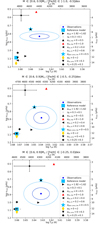 |
Fig. 4. Location of the AGBb in the plane log Teff; log νmax, in the mass bin, M ∈ [0.6, 0.9] M⊙, and metallicity bins, [Fe/H] ∈ [ − 1.0, −0.5], [ − 0.5, −0.25], [ − 0.25, 0.0] dex. The metallicity bin [Fe/H] ∈ [0.0, 0.25] dex is missing because we do not have enough stars to perform a statistically sound study. Observations are marked by blue dots, while the dark blue and light blue ellipses correspond to the 1σ and 2σ regions, respectively. The reference model presented is shown by a light blue square. Other models are shown with different symbols listed in the labels; they have been obtained by individually changing the parameters of the reference model. The changes are indicated in the label of each panel. The black dot with errorbars indicates the mean uncertainty we have for all models. The uncertainty on the AGBb location in log νmax and log Teff for each model is taken as the standard deviation of the Gaussian function that reproduces the overdensity caused by the AGBb in the 1D histograms. The numerical values are listed in Table A.1. Ranges of the axes vary in the different panels. |
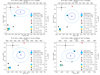 |
Fig. 5. Location of the AGBb in the plane log Teff; log νmax, in the mass bin, M ∈ [0.9, 1.2] M⊙, and metallicity bins, [Fe/H] ∈ [ − 1.0, −0.5], [ − 0.5, −0.25], [ − 0.25, 0.0], [0.0, 0.25] dex. The label is the same as in Fig. 4. The numerical values are listed in Table A.2. Ranges of the axes vary in the different panels. |
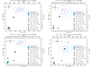 |
Fig. 6. Location of the AGBb in the plane log Teff; log νmax, in the mass bin, M ∈ [1.2, 1.5] M⊙, and metallicity bins, [Fe/H] ∈ [ − 1.0, −0.5], [ − 0.5, −0.25], [ − 0.25, 0.0], [0.0, 0.25] dex. The label is the same as in Fig. 5. The numerical values are listed in Table A.3. Ranges of the axes vary in the different panels. |
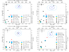 |
Fig. 7. Location of the AGBb in the plane log Teff; log νmax, in the mass bin, M ∈ [1.5, 2.5] M⊙, and metallicity bins, [Fe/H] ∈ [ − 1.0, −0.5], [ − 0.5, −0.25], [ − 0.25, 0.0], [0.0, 0.25] dex. The label is the same as in Fig. 5. An additional model represented by a black cross was computed to explore the effects of rotation by taking the rotation rate ΩZAMS/Ωcrit = 0.3 during the main sequence, relative to the reference model, where Ωcrit is the surface critical angular velocity for the star to be dislocated. Another model, labelled ‘test’ and represented by a black pentagon, was also computed to check if combining several changes could allow us to reproduce the observations. With respect to the reference model, these changes are the adding of rotation ΩZAMS/Ωcrit = 0.3, He-core overshooting αov, He = 1.0, the removal of H-core overshooting αov, H = 0.2 → 0, and the decrease of αMLT = 1.92 → 1.62. The numerical values are listed in Table A.4. We caution that the range of the axes are not the same between panels. |
5.1. AGBb seen from observations
Based on observations, we can highlight a clear mass dependence in the AGBb location: the higher the mass, the lower the νmax associated to the AGBb, whatever the range of metallicity (see left panel of Fig. 3). In particular, the higher the mass, the farther the distance between the AGBb and the clump phase along the evolutionary track. We find the AGBb to occur around log νmax ∼ 0.84 (νmax ∼ 6.9 μHz) at M ∼ 1 M⊙ and log νmax ∼ 0.52 (νmax ∼ 3.3 μHz) at M ∼ 2 M⊙, with a typical standard deviation of σ2 = 0.06 and uncertainty on the log νmax measurements of σlog νmax = 0.02. According to seismic scaling relations, the luminosity L depends on νmax, following
 (8)
(8)
Then, the higher the mass, the higher the luminosity, which is in full agreement with theoretical predictions since the AGBb luminosity was found to increase with mass at fixed metallicity (Alves & Sarajedini 1999, their Fig. 3). This behaviour was also found by Yu et al. (in prep.), who observed that the overdensity of stars associated to the AGBb is shifted between Kepler, APOGEE, and GALAH stars. This overdensity shift is correlated with a shift of the stellar mass distribution, resulting in a different mean stellar mass in those samples.
In addition, we note that in the right panel of Fig. 3, the AGBb occurs at lower temperature for high-mass stars (around log Teff ∼ 3.630 at M ∼ 1 M⊙ and log Teff ∼ 3.610 at M ∼ 2 M⊙). Although this temperature dependence is clear in Fig. 3, it may be subject to the uncertainty on the log Teff measurements of σlog Teff = 0.01 − 0.02 as well as our ability to precisely delimit the overdensity, with a standard deviation of σ2 = 0.01 − 0.02.
Beyond that mass dependence, we can see in Fig. 3 a weak metallicity effect on the AGBb location in νmax. At fixed mass, the AGBb location in νmax slowly increases with metallicity at low mass (M ≤ 1.2 M⊙) and noticeably increases at high mass (M ≥ 1.2 M⊙). This observational trend is consistent with the theoretical results of Alves & Sarajedini (1999). Indeed, for low-mass stars (M ≤ 1.2 M⊙), these authors showed that a change of metallicity does not highly impact the luminosity of the AGBb whereas for high-mass stars (M ≥ 1.2 M⊙) metallicity effects are more important, which is what we observe. Nevertheless, these trends are mainly valid for high-metallicity stars since our sample only contains a small number of metal-poor stars (with [Fe/H] ≤ −0.5 dex, see Table 1). In addition, we can see in Fig. 3 that the AGBb tends to occur at lower log Teff when the metallicity increases. However, the log Teff variations with metallicity are close to the typical uncertainty on log Teff, so this behaviour needs to be confirmed. Overall, our results tend to confirm that the AGBb occurrence slightly depends on the metallicity that would make the use of AGBb as standard candle questionable (Pulone 1992; Ferraro 1992) – at least at high metallicity. This aspect is discussed in Sect. 6.
In summary, we find a clear mass dependence of the AGBb location, whereby the higher the mass, the lower νmax and Teff at which the AGBb occurs, thus, the later the AGBb occurrence. Moreover, the AGBb tends to occur at slightly higher νmax and lower Teff for metal-rich stars.
5.2. Necessity for calibrating the core overshooting parameter
In order to estimate the amount of core overshooting αov, He needed to reproduce the observations, we computed evolutionary tracks without core overshooting (αov, He = 0). In Figs. 4−7, we can see that the AGBb locations in observations and models without core overshooting during the clump phase do not overlap at all, neither in the M − [Fe/H] − log νmax nor in the M − [Fe/H] − log Teff plane. However, we notice that for a given set of stellar parameters, the greater the mass, the larger the differences between observations and models in νmax and Teff at the AGBb. This is also what we observe toward low metallicity, but only in Teff. As highlighted in Sect. 5.1 and in theoretical works (Alves & Sarajedini 1999, their Fig. 3), the metallicity effects are small but still impacts the frequency νmax at which the AGBb occurs. Consequently, we can conclude that models with different masses and metallicities have to be calibrated in different ways.
Then, we adopted a moderate and high core overshooting parameter αov, He = 0.5 and 1.0, which are the values that provide the best matching of the period-spacing and luminosity distributions between observations and stellar models during He-burning phases in the range M ∈ [1.3, 1.7] M⊙ (Bossini et al. 2015). From Figs. 4−7, we can conclude that core overshooting has to take place during the core He-burning phase in order to reproduce the observations. Adding core overshooting during the clump phase increases the distance between the latter and the AGBb location along the evolutionary track, which makes the AGBb occur at lower νmax and lower Teff. We note that αov, He = 0.5 (respectively, αov, He = 1.0) gives a fine agreement between models and observations for stellar mass M ∈ [0.9, 1.2] M⊙ (respectively M ∈ [1.2, 1.5] M⊙) for all metallicities. This tends to confirm that the higher the mass, the higher the core overshooting αov, He must be for the models to agree with observations. Nevertheless, for high-mass stars adding He-core overshooting seems inadequate with regard to reproducing the observations. The value of αov, He = 1.0 in units of HP, which quantifies the extent of the mixing region beyond the boundary of convective instability, may be unrealistic since the overshooting region then becomes larger than the convective core. Consequently, the inclusion of additional physical processes may be necessary to make models and observations match at high mass.
In log Teff, the AGBb location varies with metallicity at fixed mass in stellar models (see Figs. 4−7 and Tables A.1−A.4). Therefore, other model parameters have to be fine-tuned in order to make observations and models agree both in log νmax and log Teff for all bins of metallicity. This raises the question of degeneracies and uncertainties on stellar parameters. In Sect. 6, we explore the effects of model input physics that could influence the AGBb location.
6. Discussion
6.1. Calibration of physical parameters at low mass
In Sect. 6, we explore the effects of model input physics that could influence the AGBb. Up to this point, we investigated the impact of He-core overshooting on the AGBb by taking ∇T = ∇rad in the overshooting region. Following Bossini et al. (2015), we also investigated the penetrative convection scenario defined as ∇T = ∇ad in the overshooting region. According to Figs. 4−6 there is no difference in the location of the AGBb between those two scenarios. Bossini et al. (2015) reached the same conclusion, however, Bossini et al. (2017) noted that the period-spacing distribution of He-burning stars observed by Vrard et al. (2016) more aptly matches the one obtained with a radiative transport in the overshooting region. Therefore, seismic constraints support the use of overshooting with radiative transport during core He-burning phase, without any impact on the calibration of the AGBb.
6.1.1. Convection efficiency
Besides, by changing the mixing length parameter αMLT, we noted that the convection efficiency considerably impacts the AGBb location in Teff. In Figs. 4−6, we can see that a ΔαMLT decrease of 0.3 induces a shift of the AGBb toward low Teff, but it only marginally modifies its luminosity. In fact, when the mixing length parameter decreases, the energy transport in the envelope is less efficient, the stellar radius R increases and the effective temperature Teff decreases. Then, the evolutionary track is shifted toward low Teff, including the AGBb location. On the other hand, by considering the scaling relation:
 (9)
(9)
we see that at fixed mass, increasing the radius R and decreasing the effective temperature, Teff, simultaneously has limited effect on νmax, which justifies the minor impact of ΔαMLT on the AGBb location in νmax.
6.1.2. Other model inputs
We checked that some physical mechanisms do not modify the AGBb location, which are summarised as follows: (1) Modifying the H-core overshooting αov, H during the MS does not shift the AGBb location for low-mass stars (M ≤ 1.5 M⊙) since their convective core is either not developed yet or very small. (2) Interestingly, adding an amount of envelope undershooting of αov, env = 0.3 HP (i.e. overshooting from the convective envelope into the radiative core) from the main sequence up to the AGB does not impact the AGBb location, while it does impact the RGBb location (Khan et al. 2018). This implies that the calibrations of mixing processes brought by the RGBb (envelope undershooting) and AGBb (He-core overshooting) are independent. (3) On the other hand, adding thermohaline convection from the main sequence up to the early AGB with αth = 2 marginally modifies the AGBb location. Mixing processes between the convective envelope and the radiative core do not seem to significantly impact the AGBb. (4) Changing the mass loss rate on the RGB from ηR = 0.3 to ηR = 0.1 slightly shifts the AGBb location. This suggests that the changes the star experienced due to mass loss do not impact the AGBb occurrence. It is only the final mass reached at the AGBb that matters when determining the AGBb location. (5) By varying the initial helium mass fraction from Y0 = 0.253 to Y0 = 0.303, the AGBb occurs at slightly lower νmax, namely, at higher luminosity. This is consistent with the expectations since an increased initial helium mass fraction extends the lifetime of the core He-burning phase. Thus, more thermonuclear energy is released, and then the luminosity is higher at this evolutionary stage.
In conclusion, we are able to reproduce the AGBb location of low-mass stars with stellar models, in particular, by including He-core overshooting αov, He, as investigated by Bossini et al. (2015). We find that a helium core overshooting parameter αov, He ∈ [0.25, 0.50] is needed to make the observations and models match in the mass bins M ∈ [0.6, 0.9],[0.9, 1.2] M⊙, while αov, He ∈ [0.50, 1.0] is more appropriate in the mass bin M ∈ [1.2, 1.5] M⊙. Deviations of models from the observations in Teff can be captured by adjusting the mixing length parameter αMLT. The main sources of uncertainty on the calibration of He-core overshooting come from the initial helium mass fraction and potential other mixing processes such as rotational mixing. Additional observational constraints could be used to reduce these uncertainties, particularly with regard to the location of the red clump phase. The physical parameter changes we explored also have an impact on the location of the red clump phase, so combining the observed AGBb location with that of the red clump phase would lead to a more precise calibration. In Appendix B, we explore how physical ingredients impact the ratio of location in log νmax and log Teff between the AGBb and the red clump phase. We note that only the addition of He-core overshooting modifies the distance between the AGBb and the red clump locations along the evolutionary track, while the other parameters leave this distance unchanged. Some parameters not only have an effect on the AGBb location but also on the red clump location, such as the initial helium abundance. Additional work is required to improve the calibration of the simultaneous investigations of the red clump and AGBb locations. On the other hand, we did not explore rotation-induced mixing in low-mass stars since physical ingredients such as surface magnetic braking (Ekström et al. 2012) are missing to correctly model rotational mixing in low-mass stars (M ≤ 1.5 M⊙) in the default MESA files.
6.2. Calibration of physical parameters at high mass
The locations of the AGBb derived from observations and stellar models are represented in Fig. 7 for high-mass stars. Modifying the reference model in a similar way as for low-mass stars leads to the same effects highlighted in Sect. 5.2. Adding He-core overshooting increases the distance between the AGBb occurrence and the core He-burning phase along the evolutionary track, decreasing the mixing length parameter αMLT makes the AGBb occur at lower Teff; then, modifying the other parameters does not significantly impact the AGBb location – except for the H-core overshooting parameter. Indeed, for stellar masses above 1.5 M⊙, the convective core during the main sequence is sufficiently developed so that H-core overshooting can occur. In Fig. 7, it can be seen that increasing αov, H from 0.2 to 0.6 has roughly the same effect on the AGBb location as adding He-core overshooting αov, He = 0.5. Nevertheless, a high efficiency of H-core overshooting appears to be unrealistic considering the latest values calibrated with observational constraints in eclipsing binaries (e.g. Claret & Torres 2016, 2017, 2018, 2019), which do not exceed αov, H ∼ 0.2. Similarly, values of αov, H lower than 0.2 have been derived from the calibration of dipole modes in low-mass stars by Deheuvels et al. (2016). Finally, recent theoretical predictions based on 3D numerical hydrodynamics simulations of penetrative convection also give αov, H < 0.2 for masses M < 3 M⊙ (Anders et al. 2022; Jermyn et al. 2022). The additional effects of this unrealistic H-core overshooting can be mimicked by taking into account additional mixing processes at work between the convective core and the radiative core. For instance, we found that adding rotational mixing during the main sequence with a rotation rate of ΩZAMS/Ωcrit = 0.3 roughly produces the same changes in the AGBb location (see Fig. 7, for the metallicity bins [Fe/H] ∈ [ − 0.25, 0.0], [0.0, 0.25] dex).
None of the physical mechanisms added to the reference model is enough to reproduce observations. Even the model closest to observations that is obtained by adding a high He-core overshooting cannot reproduce the observed AGBb location. Choosing a higher efficiency of He-core overshooting may be unrealistic since the extent of the extra mixing region would be even higher than that of the convective core, but it suggests that additional mixing processes are needed to match the models and observations. To investigate those effects a bit further, we combined the two mixing processes that mostly impact the AGBb location, namely, core overshooting during the core He-burning phase and rotational mixing during the main sequence, and we added them to the reference model. As illustrated in Fig. 7, by (1) adding rotational mixing with a rotation rate of ΩZAMS/Ωcrit = 0.3; (2) adding He-core overshooting αov, He = 1.0; (3) then taking H-core overshooting away, via αov, H = 0, and decreasing the mixing length parameter of ΔαMLT = 0.3, we are able to reproduce the observed AGBb location.
In summary, several mixing processes such as rotational mixing and He-core overshooting need to be simultaneously taken into account and calibrated to reproduce observations of high-mass stars. However, rotational mixing during the main sequence remains exploratory and further work is required to quantify its significance relative to other mixing processes such as He-core overshooting.
6.3. AGBb as a distance indicator
In Sect. 5.1, we noted that the AGBb location in νmax slightly changes with metallicity at fixed mass, especially for high-mass stars, which implies that the luminosity at the AGBb varies with metallicity. This agrees with the theoretical results of Alves & Sarajedini (1999), where the AGBb luminosity is expected to significantly vary with metallicity, especially for high-mass stars with M ≥ 1.2 M⊙. At first glance, our conclusions seem to be in disagreement with the results of the models of Pulone (1992) and Ferraro (1992), as these authors justified the use of the AGBb as a standard candle by its independence from metallicity. However, these studies are based on a sample of low-metallicity stars in Galactic globular clusters with [Fe/H] ≲ −0.5 dex, while ours is mainly composed of high-metallicity stars with [Fe/H] ≳ −0.5 dex (see Table 1). This tends to confirm that the AGBb location changes at high metallicity. Therefore, metal-rich AGBb stars cannot be used as standard candles. However, this behaviour needs further inspections at low metallicity. We do not have a large enough number of metal-poor AGB stars with [Fe/H] < −0.75 dex to create additional metallicity bins, which limits the analysis of the metallicity dependence of the AGBb. A larger sample of stars would be desirable to confirm or refute this metallicity dependence at low metallicity. In parallel, it could be interesting to evaluate the potential of the AGBb as a distance indicator and to test whether any metallicity bias is identifiable.
7. Conclusion
With the excellent precision of photometric data collected by Kepler and TESS, we are now able to perform asteroseismic studies of high-luminosity red giants. This offers access to oscillation mode properties of those stars, which can be used to constrain stellar interiors. In this work, we take advantage of the νmax estimates from Kepler and TESS targets and combined them with spectroscopic data to characterise the AGBb in the widest range and most resolved bins of mass and metallicity explored thus far. This would not have been possible without combining targets from several catalogues, given the small number of evolved giants subject to a seismic study and the uncertainties on the classification methods between RGB and AGB stars. We detected and accurately located the AGBb in the log Teff − log νmax plane, using a statistical method to distinguish stars belonging to the AGBb and to the AGB background. We highlighted that the occurrence of the AGBb depends on the stellar mass: it clearly takes place at lower νmax (i.e. at higher luminosity) and occurs within uncertainty at cooler temperature for high-mass stars, in agreement with theoretical models. In parallel, the dependence of the AGBb location on metallicity implies that using it as a standard candle requires some care.
Furthermore, we were able to use the AGBb location in the log Teff − log νmax plane as a constraint for parameters in stellar models in limited bins of mass and metallicity. It is mainly the mixing-length parameter and mixing processes such as He-core overshooting that affect the location of the AGBb. Some stellar parameters do not affect the AGBb location (or they do so only slightly), such as the initial helium abundance Y0, the mass-loss rate on the RGB ηR, the envelope undershooting αov, env, and the thermohaline convection, αth. Those stellar parameters contribute to the uncertainty of the calibration of mixing processes to match observations. We confirmed that models without core overshooting during the core He-burning phase cannot reproduce observations, as already shown in Bossini et al. (2015). Moreover, we reported that the amount of He-core overshooting needed to match the observations and models depends on the stellar mass, and increases along with it. Indicatively, the core overshooting value αov, He ∈ [0.25, 0.50] aptly suits the observations for stars with M ∈ [0.6, 1.2] M⊙, while αov, He ∈ [0.5, 1.0] more aptly suits those for stars with M ∈ [1.2, 1.5] M⊙. However, for high-mass stars M ≥ 1.5 M⊙, modifying the He-core overshooting only does not allow us to reproduce observations. In this case, we explored additional mixing processes, especially rotational mixing during the main sequence, and we found that we could match models and observations by combining rotation-induced mixing and He-core overshooting. Further work is needed to investigate the possible degeneracy between those mixing processes at high mass and to quantify their weight.
The core overshooting calibration does also depend on the metallicity, but not as strongly as the mass in terms of log νmax, which makes the values previously cited well suited to all bins of metallicity studied. However, because the AGBb location in log Teff varies with metallicity among the models, we need to calibrate other parameters, such as the mixing-length parameter, αMLT, in stellar models so that the observations and stellar models can be matched in log Teff and log νmax at the same time.
In the future, new space-borne missions will be helpful in filling the sample of evolved red giants targets, hence, to take into account more low-metallicity stars ([Fe/H] ≤ −0.5 dex) and high-mass stars (M ≥ 1.5 M⊙). This will give us the opportunity to improve the precision on the observed AGBb location for those bins of mass and metallicity where we lack asteroseismic and spectroscopic data. In addition, it will confirm or disprove the potential of the AGBb as a suitable standard candle.
This correction is applied to capture the deviations from the asteroseismic scaling relations between the stellar mass, M, radius, R, large frequency separation, Δν, and frequency at maximum oscillation power, νmax.
Z/X = (Z/X)⊙ 10[Fe/H], where the solar value (Z/X)⊙ = 0.0181 is taken from Asplund et al. (2009).
This value corresponds to the default solar age in MESA, taken as the sum of the time spent on the MS starting on the ZAMS (4.57 × 10⁹ yr) and that spent on the PMS (0.04 × 10⁹ yr). It is larger than the value commonly adopted τ⊙ = 4.57 × 10⁹ yr (see, e.g., Chaussidon 2007). However, we do not account for the PMS in the calibration and it has been shown that adopting those two target solar ages does not impact the solar calibration significantly (see Table 2 of Sackmann et al. 1990).
Acknowledgments
The authors are grateful to the anonymous referee who helped them in improving this paper with constructive suggestions. G.D. thanks S. Khan and O. Hall for their valuable suggestions that helped improving this work. D.B. acknowledges supported by FCT through the research grants UIDB/04434/2020, UIDP/04434/2020 and PTDC/FIS-AST/30389/2017, and by FEDER-Fundo Europeu de Desenvolvimento Regional through COMPETE2020-Programa Operacional Competitividade e Internacionalização (grant: POCI-01-0145-FEDER-030389).
References
- Abdurro’uf, Accetta, K., Aerts, C., et al. 2022, ApJS, 259, 35 [NASA ADS] [CrossRef] [Google Scholar]
- Alves, D. R., & Sarajedini, A. 1999, ApJ, 511, 225 [NASA ADS] [CrossRef] [Google Scholar]
- Anders, E. H., Jermyn, A. S., Lecoanet, D., & Brown, B. P. 2022, ApJ, 926, 169 [NASA ADS] [CrossRef] [Google Scholar]
- Angulo, C., Arnould, M., Rayet, M., et al. 1999, Nucl. Phys. A, 656, 3 [Google Scholar]
- Asplund, M., Grevesse, N., Sauval, A. J., & Scott, P. 2009, ARA&A, 47, 481 [NASA ADS] [CrossRef] [Google Scholar]
- Baudin, F., Barban, C., Goupil, M. J., et al. 2012, A&A, 538, A73 [NASA ADS] [CrossRef] [EDP Sciences] [Google Scholar]
- Benomar, O., Belkacem, K., Bedding, T. R., et al. 2014, ApJ, 781, L29 [Google Scholar]
- Blocker, T. 1995, A&A, 297, 727 [Google Scholar]
- Bono, G., Castellani, V., degl’Innocenti, S., & Pulone, L. 1995, A&A, 297, 115 [NASA ADS] [Google Scholar]
- Bossini, D., Miglio, A., Salaris, M., et al. 2015, MNRAS, 453, 2290 [Google Scholar]
- Bossini, D., Miglio, A., Salaris, M., et al. 2017, MNRAS, 469, 4718 [Google Scholar]
- Buder, S., Sharma, S., Kos, J., et al. 2021, MNRAS, 506, 150 [NASA ADS] [CrossRef] [Google Scholar]
- Cantiello, M., & Langer, N. 2010, A&A, 521, A9 [NASA ADS] [CrossRef] [EDP Sciences] [Google Scholar]
- Caputo, F., Castellani, V., & Wood, P. R. 1978, MNRAS, 184, 377 [NASA ADS] [Google Scholar]
- Cassisi, S., Potekhin, A. Y., Pietrinferni, A., Catelan, M., & Salaris, M. 2007, ApJ, 661, 1094 [NASA ADS] [CrossRef] [Google Scholar]
- Castellani, V., Giannone, P., & Renzini, A. 1971a, Ap&SS, 10, 355 [NASA ADS] [CrossRef] [Google Scholar]
- Castellani, V., Giannone, P., & Renzini, A. 1971b, Ap&SS, 10, 340 [NASA ADS] [CrossRef] [Google Scholar]
- Castellani, V., Chieffi, A., & Pulone, L. 1991, ApJS, 76, 911 [NASA ADS] [CrossRef] [Google Scholar]
- Caughlan, G. R., & Fowler, W. A. 1988, At. Data Nucl. Data Tab., 40, 283 [NASA ADS] [CrossRef] [Google Scholar]
- Charbonnel, C., & Zahn, J. P. 2007, A&A, 467, L15 [NASA ADS] [CrossRef] [EDP Sciences] [Google Scholar]
- Chaussidon, M. 2007, in Lectures in Astrobiology, eds. M. Gargaud, H. Martin, & P. Claeys, 45 [CrossRef] [Google Scholar]
- Chiosi, C. 2007, in Convection in Astrophysics, eds. F. Kupka, I. Roxburgh, & K. L. Chan, 239, 235 [NASA ADS] [Google Scholar]
- Chugunov, A. I., Dewitt, H. E., & Yakovlev, D. G. 2007, Phys. Rev. D, 76, 025028 [NASA ADS] [CrossRef] [Google Scholar]
- Claret, A., & Torres, G. 2016, A&A, 592, A15 [NASA ADS] [CrossRef] [EDP Sciences] [Google Scholar]
- Claret, A., & Torres, G. 2017, ApJ, 849, 18 [Google Scholar]
- Claret, A., & Torres, G. 2018, ApJ, 859, 100 [Google Scholar]
- Claret, A., & Torres, G. 2019, ApJ, 876, 134 [Google Scholar]
- Deheuvels, S., Brandão, I., Silva Aguirre, V., et al. 2016, A&A, 589, A93 [NASA ADS] [CrossRef] [EDP Sciences] [Google Scholar]
- di Mauro, M. P., Cardini, D., Catanzaro, G., et al. 2011, MNRAS, 415, 3783 [NASA ADS] [CrossRef] [Google Scholar]
- Dréau, G., Mosser, B., Lebreton, Y., Gehan, C., & Kallinger, T. 2021, A&A, 650, A115 [NASA ADS] [CrossRef] [EDP Sciences] [Google Scholar]
- Eggleton, P. P., Dearborn, D. S. P., & Lattanzio, J. C. 2006, Science, 314, 1580 [Google Scholar]
- Eggleton, P. P., Dearborn, D. S. P., & Lattanzio, J. C. 2008, ApJ, 677, 581 [NASA ADS] [CrossRef] [Google Scholar]
- Ekström, S., Georgy, C., Eggenberger, P., et al. 2012, A&A, 537, A146 [Google Scholar]
- Elsworth, Y., Themeßl, N., Hekker, S., & Chaplin, W. 2020, Res. Notes Am. Astron. Soc., 4, 177 [Google Scholar]
- Endal, A. S., & Sofia, S. 1978, ApJ, 220, 279 [NASA ADS] [CrossRef] [Google Scholar]
- Ferraro, F. R. 1992, Mem. Soc. Astron. It., 63, 491 [Google Scholar]
- Foreman-Mackey, D. 2016, J. Open Sour. Softw., 1, 24 [NASA ADS] [CrossRef] [Google Scholar]
- Foreman-Mackey, D., Hogg, D. W., Lang, D., & Goodman, J. 2013, PASP, 125, 306 [Google Scholar]
- Fynbo, H. O. U., Diget, C. A., Bergmann, U. C., et al. 2005, Nature, 433, 136 [Google Scholar]
- Heger, A., Langer, N., & Woosley, S. E. 2000, ApJ, 528, 368 [NASA ADS] [CrossRef] [Google Scholar]
- Henyey, L., Vardya, M. S., & Bodenheimer, P. 1965, ApJ, 142, 841 [Google Scholar]
- Herwig, F., Blöcker, T., & Driebe, T. 2000, Mem. Soc. Astron. It., 71, 745 [Google Scholar]
- Hogg, D. W., Bovy, J., & Lang, D. 2010, ArXiv e-prints [arXiv:1008.4686] [Google Scholar]
- Huang, W., Gies, D. R., & McSwain, M. V. 2010, ApJ, 722, 605 [Google Scholar]
- Iglesias, C. A., & Rogers, F. J. 1996, ApJ, 464, 943 [NASA ADS] [CrossRef] [Google Scholar]
- Imbriani, G., Costantini, H., Formicola, A., et al. 2004, A&A, 420, 625 [NASA ADS] [CrossRef] [EDP Sciences] [Google Scholar]
- Jermyn, A. S., Anders, E. H., Lecoanet, D., & Cantiello, M. 2022, ApJ, 929, 182 [NASA ADS] [CrossRef] [Google Scholar]
- Kallinger, T., Hekker, S., Mosser, B., et al. 2012, A&A, 541, A51 [NASA ADS] [CrossRef] [EDP Sciences] [Google Scholar]
- Kawaler, S. D. 1988, ApJ, 333, 236 [Google Scholar]
- Khan, S., Hall, O. J., Miglio, A., et al. 2018, ApJ, 859, 156 [NASA ADS] [CrossRef] [Google Scholar]
- Kippenhahn, R., Ruschenplatt, G., & Thomas, H. C. 1980, A&A, 91, 175 [Google Scholar]
- Kjeldsen, H., & Bedding, T. R. 1995, A&A, 293, 87 [NASA ADS] [Google Scholar]
- Knapp, G. R., Young, K., Lee, E., & Jorissen, A. 1998, ApJS, 117, 209 [CrossRef] [Google Scholar]
- Lagarde, N., Miglio, A., Eggenberger, P., et al. 2015, A&A, 580, A141 [NASA ADS] [CrossRef] [EDP Sciences] [Google Scholar]
- Langer, N., El Eid, M. F., & Fricke, K. J. 1985, A&A, 145, 179 [NASA ADS] [Google Scholar]
- Mackereth, J. T., Miglio, A., Elsworth, Y., et al. 2021, MNRAS, 502, 1947 [NASA ADS] [CrossRef] [Google Scholar]
- Maeder, A. 1975, A&A, 40, 303 [NASA ADS] [Google Scholar]
- Marigo, P., & Aringer, B. 2009, A&A, 508, 1539 [CrossRef] [EDP Sciences] [Google Scholar]
- Marigo, P., & Girardi, L. 2007, A&A, 469, 239 [NASA ADS] [CrossRef] [EDP Sciences] [Google Scholar]
- Mathur, S., García, R. A., Régulo, C., et al. 2010, A&A, 511, A46 [NASA ADS] [CrossRef] [EDP Sciences] [Google Scholar]
- Mauron, N., & Huggins, P. J. 2006, A&A, 452, 257 [NASA ADS] [CrossRef] [EDP Sciences] [Google Scholar]
- McDonald, I., & Trabucchi, M. 2019, MNRAS, 484, 4678 [Google Scholar]
- McDonald, I., De Beck, E., Zijlstra, A. A., & Lagadec, E. 2018, MNRAS, 481, 4984 [NASA ADS] [CrossRef] [Google Scholar]
- Meynet, G., & Maeder, A. 1997, A&A, 321, 465 [NASA ADS] [Google Scholar]
- Miglio, A., Chiappini, C., Mackereth, J. T., et al. 2021, A&A, 645, A85 [NASA ADS] [CrossRef] [EDP Sciences] [Google Scholar]
- Mosser, B., & Appourchaux, T. 2009, A&A, 508, 877 [NASA ADS] [CrossRef] [EDP Sciences] [Google Scholar]
- Mosser, B., Dziembowski, W. A., Belkacem, K., et al. 2013, A&A, 559, A137 [CrossRef] [EDP Sciences] [Google Scholar]
- Mosser, B., Benomar, O., Belkacem, K., et al. 2014, A&A, 572, L5 [NASA ADS] [CrossRef] [EDP Sciences] [Google Scholar]
- Mosser, B., Michel, E., Samadi, R., et al. 2019, A&A, 622, A76 [NASA ADS] [CrossRef] [EDP Sciences] [Google Scholar]
- Paxton, B., Bildsten, L., Dotter, A., et al. 2011, ApJS, 192, 3 [Google Scholar]
- Paxton, B., Cantiello, M., Arras, P., et al. 2013, ApJS, 208, 4 [Google Scholar]
- Paxton, B., Marchant, P., Schwab, J., et al. 2015, ApJS, 220, 15 [Google Scholar]
- Paxton, B., Schwab, J., Bauer, E. B., et al. 2018, ApJS, 234, 34 [NASA ADS] [CrossRef] [Google Scholar]
- Paxton, B., Smolec, R., Schwab, J., et al. 2019, ApJS, 243, 10 [Google Scholar]
- Pinçon, C., Goupil, M. J., & Belkacem, K. 2020, A&A, 634, A68 [Google Scholar]
- Pinsonneault, M. H., Kawaler, S. D., Sofia, S., & Demarque, P. 1989, ApJ, 338, 424 [Google Scholar]
- Pinsonneault, M. H., Elsworth, Y., Epstein, C., et al. 2014, ApJS, 215, 19 [Google Scholar]
- Pinsonneault, M. H., Elsworth, Y. P., Tayar, J., et al. 2018, ApJS, 239, 32 [Google Scholar]
- Pulone, L. 1992, Mem. Soc. Astron. It., 63, 485 [Google Scholar]
- Ramstedt, S., Schöier, F. L., Olofsson, H., & Lundgren, A. A. 2008, A&A, 487, 645 [NASA ADS] [CrossRef] [EDP Sciences] [Google Scholar]
- Reimers, D. 1975, Mem. Soc. R. Sci. Liege, 8, 369 [NASA ADS] [Google Scholar]
- Robertson, J. W., & Faulkner, D. J. 1972, ApJ, 171, 309 [NASA ADS] [CrossRef] [Google Scholar]
- Sackmann, I. J., Boothroyd, A. I., & Fowler, W. A. 1990, ApJ, 360, 727 [NASA ADS] [CrossRef] [Google Scholar]
- Salaris, M., & Cassisi, S. 2017, R. Soc. Open Sci., 4, 170192 [Google Scholar]
- Steinmetz, M., Guiglion, G., McMillan, P. J., et al. 2020, AJ, 160, 83 [NASA ADS] [CrossRef] [Google Scholar]
- Stello, D., Compton, D. L., Bedding, T. R., et al. 2014, ApJ, 788, L10 [NASA ADS] [CrossRef] [Google Scholar]
- Sweigart, A. V., & Gross, P. G. 1973, BAAS, 5, 314 [NASA ADS] [Google Scholar]
- Ulrich, R. K. 1972, ApJ, 172, 165 [NASA ADS] [CrossRef] [Google Scholar]
- Vrard, M., Mosser, B., & Samadi, R. 2016, A&A, 588, A87 [CrossRef] [EDP Sciences] [Google Scholar]
- Wagstaff, G., Miller Bertolami, M. M., & Weiss, A. 2020, MNRAS, 493, 4748 [Google Scholar]
- Yu, J., Bedding, T. R., Stello, D., et al. 2020, MNRAS, 493, 1388 [Google Scholar]
- Yu, J., Hekker, S., Bedding, T. R., et al. 2021, MNRAS, 501, 5135 [NASA ADS] [CrossRef] [Google Scholar]
- Zahn, J. P. 1991, A&A, 252, 179 [Google Scholar]
Appendix A: Effects of stellar parameters on the AGBb occurrence
The AGBb locations in log Teff and log νmax, presented in Figs. 4, 5, 6, and 7 in the mass bins M ∈ [0.6, 0.9], [0.9, 1.2], [1.2, 1.5], and [1.5, 2.5]M⊙ as well as metallicity bins [Fe/H] ∈[−1.0, −0.5], [ − 0.5, −0.25], [ − 0.25, 0.0], and [0.0, 0.25] dex, are summarised in Tables A.1, A.2, A.3, and A.4.
AGBb location for observations and models with M ∈ [0.6, 0.9]M⊙.
AGBb location for observations and models with M ∈ [0.9, 1.2]M⊙.
AGBb location for observations and models with M ∈ [1.2, 1.5]M⊙.
AGBb location for observations and models with M ∈ [1.5, 2.5]M⊙.
Appendix B: Distance between the AGBb and clump phase
Another relevant property of the AGBb to investigate is the distance in log νmax and log Teff between its location and that of the core He-burning phase. Indeed, theoretical models report a weak dependence of the luminosity ratio between the AGBb and red clump locations on the metallicity and initial helium abundance (Castellani et al. 1991; Bono et al. 1995). Accordingly, we inspected how the ratio of log νmax and log Teff between the AGBb and red clump phase varies with a change in physical parameters. To this end, we needed to extract the location of the red clump. We proceeded in the same way as described in Sect. 4.2, but we adapted this approach for the overdensity of stars in the clump phase. We only included stellar models for which the core helium abundance lies in the interval Yc ∈ [0.01, 0.95] in the histogram. Then, we extracted the clump location independently from that of the AGBb. The ratios in log νmax and log Teff between the AGBb and the red clump phase for our set of stellar models are shown in Tables B.1, B.2, B.3, and B.4.
Ratio between the AGBb location and the clump location for models with M ∈ [0.6, 0.9]M⊙.
Ratio between the AGBb location and the clump location for models with M ∈ [0.9, 1.2]M⊙.
Ratio between the AGBb location and the clump location for models with M ∈ [1.2, 1.5]M⊙.
Ratio between the AGBb location and the clump location for models with M ∈ [1.5, 2.5]M⊙.
Overall, the ratio in log Teff is almost constant and the ratio in log νmax weakly decreases (equivalently, the ratio in log L weakly increases) when the metallicity increases with a given set of physical ingredients. This is in agreement with the typical difference between metal-poor and metal-rich models obtained with the theoretical models of Castellani et al. (1991, their Fig. 7). These ratios do not significantly change within uncertainties when a specific change in a physical parameter is performed, except in the case when He-core overshooting is added. Indeed, both ratios in log νmax and log Teff substantially decrease (namely the ratio in log L increases) when adding He-core overshooting. This implies that the adding of He-core overshooting causes an increase in the distance between the AGBb and the red clump locations along the evolutionary track, but a change in other physical parameters leave this distance constant.
Given that some physical ingredients have an effect on the AGBb location but leave the ratio of location between the AGBb and the red clump unchanged, it means that some of those physical ingredients also impact the red clump location. This is not surprising with regard to the physical parameters such as the initial helium abundance, as it determines how much helium burning contributes to the stellar luminosity during the red clump phase. Consequently, this ratio in log νmax could also be used in combination with the AGBb location in log νmax as calibrators for mixing processes to reproduce both the AGBb and the red clump locations in the same time.
All Tables
Ratio between the AGBb location and the clump location for models with M ∈ [0.6, 0.9]M⊙.
Ratio between the AGBb location and the clump location for models with M ∈ [0.9, 1.2]M⊙.
Ratio between the AGBb location and the clump location for models with M ∈ [1.2, 1.5]M⊙.
Ratio between the AGBb location and the clump location for models with M ∈ [1.5, 2.5]M⊙.
All Figures
|
Fig. 1. Seismic HR diagram of our sample of stars in the bin of mass, M ∈ [0.9, 1.2] M⊙ (left) and in the bin of metallicity, [Fe/H] ∈ [ − 0.25, 0.0] dex (right). In both panels, stars with different metallicities (left) and masses (right) are represented with different colours. On top of those observations, stellar evolutionary tracks along the AGB are represented with black lines at different metallicities at 1 M⊙ (left) and masses at [Fe/H] = −0.25 dex (right). |
| In the text | |
|
Fig. 2. Probability distribution functions of our data set in the log Teff; log νmax plane, in the bins M ∈ [0.9, 1.2] M⊙ and [Fe/H] ∈ [ − 0.25, 0.0] dex. Upper left panel: 2D histogram where the AGBb is located by a blue diamond. Dark blue and light blue ellipses correspond to the 1σ and 2σ regions of the bivariate Gaussian, respectively. The red dashed line reproduces the linear term belonging to the RGB/AGB background. Upper right panel: normalised 1D histogram in log νmax is shown in black. The ordinate axis is the same as in the upper left panel. The blue line corresponds to the probability distribution function made of the Gaussian associated to the overdensity in log νmax, multiplied by the rising exponential in log νmax. Lower left panel: same label as in the upper right panel but in terms of log Teff. The abscissa axis is the same as in the upper left panel. The blue line shows the Gaussian associated to the overdensity in log Teff. Lower right panel: difference between log νmax and abglog Teff + bbg. The blue line illustrates the normal distribution around the linear term. |
| In the text | |
|
Fig. 3. Location of the AGBb in log νmax (left) and in log Teff (right) from observations, as a function of the metallicity, [Fe/H]. The AGBb occurrence is marked by dots and the stellar mass is colour-coded. AGBb locations obtained in the same bin of mass, M ∈ [0.6, 0.9], [0.9, 1.2], [1.2, 1.5], [1.5, 2.5] M⊙ are connected by dark blue, light blue, light green, and red lines, respectively. Mean error bars on the location of the AGBb in log νmax and in log Teff are shown in black. Data in the bin M ∈ [0.6, 0.9] M⊙; [Fe/H] ∈ [0, 0.25] dex are not shown because there are not enough stars to perform the statistical mixture model. |
| In the text | |
|
Fig. 4. Location of the AGBb in the plane log Teff; log νmax, in the mass bin, M ∈ [0.6, 0.9] M⊙, and metallicity bins, [Fe/H] ∈ [ − 1.0, −0.5], [ − 0.5, −0.25], [ − 0.25, 0.0] dex. The metallicity bin [Fe/H] ∈ [0.0, 0.25] dex is missing because we do not have enough stars to perform a statistically sound study. Observations are marked by blue dots, while the dark blue and light blue ellipses correspond to the 1σ and 2σ regions, respectively. The reference model presented is shown by a light blue square. Other models are shown with different symbols listed in the labels; they have been obtained by individually changing the parameters of the reference model. The changes are indicated in the label of each panel. The black dot with errorbars indicates the mean uncertainty we have for all models. The uncertainty on the AGBb location in log νmax and log Teff for each model is taken as the standard deviation of the Gaussian function that reproduces the overdensity caused by the AGBb in the 1D histograms. The numerical values are listed in Table A.1. Ranges of the axes vary in the different panels. |
| In the text | |
|
Fig. 5. Location of the AGBb in the plane log Teff; log νmax, in the mass bin, M ∈ [0.9, 1.2] M⊙, and metallicity bins, [Fe/H] ∈ [ − 1.0, −0.5], [ − 0.5, −0.25], [ − 0.25, 0.0], [0.0, 0.25] dex. The label is the same as in Fig. 4. The numerical values are listed in Table A.2. Ranges of the axes vary in the different panels. |
| In the text | |
|
Fig. 6. Location of the AGBb in the plane log Teff; log νmax, in the mass bin, M ∈ [1.2, 1.5] M⊙, and metallicity bins, [Fe/H] ∈ [ − 1.0, −0.5], [ − 0.5, −0.25], [ − 0.25, 0.0], [0.0, 0.25] dex. The label is the same as in Fig. 5. The numerical values are listed in Table A.3. Ranges of the axes vary in the different panels. |
| In the text | |
|
Fig. 7. Location of the AGBb in the plane log Teff; log νmax, in the mass bin, M ∈ [1.5, 2.5] M⊙, and metallicity bins, [Fe/H] ∈ [ − 1.0, −0.5], [ − 0.5, −0.25], [ − 0.25, 0.0], [0.0, 0.25] dex. The label is the same as in Fig. 5. An additional model represented by a black cross was computed to explore the effects of rotation by taking the rotation rate ΩZAMS/Ωcrit = 0.3 during the main sequence, relative to the reference model, where Ωcrit is the surface critical angular velocity for the star to be dislocated. Another model, labelled ‘test’ and represented by a black pentagon, was also computed to check if combining several changes could allow us to reproduce the observations. With respect to the reference model, these changes are the adding of rotation ΩZAMS/Ωcrit = 0.3, He-core overshooting αov, He = 1.0, the removal of H-core overshooting αov, H = 0.2 → 0, and the decrease of αMLT = 1.92 → 1.62. The numerical values are listed in Table A.4. We caution that the range of the axes are not the same between panels. |
| In the text | |
Current usage metrics show cumulative count of Article Views (full-text article views including HTML views, PDF and ePub downloads, according to the available data) and Abstracts Views on Vision4Press platform.
Data correspond to usage on the plateform after 2015. The current usage metrics is available 48-96 hours after online publication and is updated daily on week days.
Initial download of the metrics may take a while.