© W.-H. Zhou et al. 2022

1 Introduction

The unprecedented trajectory and unique spectral properties (Meech et al. 2017) exhibited during a brief visit of the first interstellar object (ISO), 1I/2017 U1 (‘Oumuamua), gave rise to a protracted controversy regarding its origin (Raymond et al. 2018b,a; Cuk 2018; Moro-Martín 2019; Zhang & Lin 2020; Jackson & Desch 2021). According to one particularly bold assumption, it is an “artificial” spacecraft with a thin light sail driven by radiation pressure on an intentional mission to our Solar System (Bialy & Loeb 2018; Loeb 2021). Based on the sensitivity limitation of the Panoramic Survey Telescope and Rapid Response System (Pan-STARRS), the interplanetary density of ‘Oumuamua-like ISOs is estimated to be n_ISO ≲ 0.2 au⁻³ in the proximity of the Earth orbit (Do et al. 2018; Trilling et al. 2017; Bannister et al. 2019). If their parent bodies randomly came across the Solar System, the inferred mass of ejected objects per star, M_ej, would exceed a few M_⊕ in the solar neighborhood (Do et al. 2018; Portegies Zwart et al. 2018). Prior to its entry into the Sun’s domain of gravitational influence, ‘Oumuamua’s velocity relative to the local standard of rest (LSR) was v_O ~ 10 km s⁻¹. At a heliocentric distance r ~ 1.5 au, its large-amplitude, irregularly varying light curve (Meech et al. 2017; Drahus et al. 2018; Bolin et al. 2017; Bannister et al. 2017; Knight et al. 2017; Jewitt et al. 2017) suggests that ‘Oumuamua is either a prolate or oblate object, freely tumbling with the period of its light curve increasing at a rate P_O ~ 0.3 h day⁻¹ from P_O ~ 8 h (Flekkøy et al. 2019). In the absence of any detectable trace of outgassing, its orbital path has an observationally inferred perihelion distance of p_O ~ 0.26 au and departs from a parabolic Keplerian trajectory with a component of nongravitational acceleration predominantly in the radial direction away from the Sun (Micheli et al. 2018), although the validity of the fitting procedure has been questioned by Katz (2019). Its surface albedo resembles that of asteroids rather than comets (Trilling et al. 2018). Shortly after ‘Oumuamua was discovered, data taken with multiple telescopes provided a high-cadence light curve (from October 25, 2017, to October 27,2017) with an irregular brightness variation over an amplitude range ~2.5–3. This high-cadence light curve has been used to deduce ‘Oumuamua’s tumbling motion (Meech et al. 2017). In addition, ‘Oumuamua was detected (Micheli et al. 2018) with magnitudes brighter than 27 in all 55 follow-up trackings (over 49 days starting on November 15, 2017).

A rationale for the spacecraft hypothesis is that it circumvents the large M_ej inferred for the parent bodies of randomly distributed ISOs. It also attributes ‘Oumuamua’s nongravitational acceleration to the Sun’s radiation pressure to a light sail under the assumption that it has a thin oblate shape with a length l₁ ~ 10² m, width l₂ ≃ l₁, surface area A, mass m_O, and surface density (Bialy & Loeb 2018) m_O/A = ρ_Ol₃ ≈ 1 kg m⁻². If ‘Oumuamua’s density, ρ_O, is comparable to that of refractory asteroids (≃2–3 × 10³ kg m⁻³), its effective thickness, l₃(~ 3–5 × 10⁻⁴m ≪ l₁) would be comparable to that of an eggshell, two orders of magnitude smaller than that of the International Space Station; although, a much thinner light sail (~ 7 × 10⁻⁶ m) has been deployed, without tumbling, on the spacecraft Interplanetary Kite-craft Accelerated by Radiation Of the Sun (IKAROS; Tsuda et al. 2011).

However, the turbulent interstellar medium (ISM) poses challenges to the navigation of the light sail. Hydrogen atoms exert a drag force that is normal to the surface of the light sail, leading to a sideways acceleration of the tumbling light sail. Moreover, in the disorderly magnetic field, B, of interstellar space, a Lorentz force in the direction (B · v_magB − |B|²v_mag)/|B|²|v_mag| is induced, which contains a drag and a sideways force component with a magnitude a_mag ~ B²v_mag/2ρ_Ol₃µ₀v_A, where v_A is the Alfvén speed in the ISM. As ‘Oumuamua passes through randomly oriented B in eddies of all sizes, L_tur, the magnitude and direction of the magnetic drag change on a timescale τ_tur ~ L_tur/v_O. On timescales t ⩾ τ_tur, the value of ‘Oumuamua’s path deviation from its initial target goes through a random walk.

Even if the light sail manages to arrive at the Solar System, the unique configuration (i.e., the extremely high dimensional ratio) of the light sail would give rise to recognizable observational features. The radiation pressure would cause a sideways acceleration due to the imperfect alignment of the surface normal vector with heliocentric position vector, which would result in a considerable non-radial deviation from Kepler motion. In addition, the tumbling of the extremely thin light sail would lead to a light curve with an immense amplitude. The light sail can even be invisible when the sunlight is edge-on to the light sail. Stringent probability assessments for the spaceship scenario can be made using ‘Oumuamua’s observed light curve and detected magnitude as well as a prefect recurrence rate.

Previous studies (e.g., Katz 2021; Curran 2021) have questioned the light-sail scenario based on the unlikely coincidence between the advancement of extraterrestrial technology and the advent of the observational capability of Pan-STARRS, though a quantitative and comprehensive analysis of observation data has not yet been performed. In this paper, we revisit the light-sail scenario with its model parameters and estimate the ram-pressure and magnetic drag and the torque on the light sail during ‘Oumuamua’s voyage through the turbulent ISM (Sect. 2). In Sect. 3, we model ‘Oumuamua’s dynamics as a tumbling light sail cruising the Solar System, and in particular we study the implications of its nongravitational acceleration due to the sideways radiation force and the observable features due to its tumbling motion and high dimensional ratio. We summarize our results and compare them with observations in Sect. 4. Lastly, we discuss our results and propose observable tests for future surveys in Sect. 5.

2 Dynamics of a tumbling light sail in interstellar space

In the solar neighborhood, the ISM contains (Draine 2010): (1) a diffuse warm neutral medium (WNM) with number density n_ISM ~ 10⁶ m⁻³ and sound speed c_s ~ 9 km s⁻¹; (2) a cold neutral medium (CNM) with n_ISM ~ 10⁸m⁻³, c_s ~ 1.3 km s⁻¹; and (3) giant molecular clouds (GMCs) with n_ISM ~ 10¹⁰–10¹² m⁻³, c_s ~ 0.5 km s⁻¹. The local volume filling factor for the WNM, the CNM, and GMCs is 0.5, 5 × 10⁻³, and 2 × 10⁻³, respectively (Draine 2010), although ‘Oumuamua may have recently traveled through some GMCs (Pfalzner et al. 2020; Hsieh et al. 2021). Due to the perturbation of GMCs, the velocity dispersion of ‘Oumuamua and nearby stars relative to the LSR v_d(τ„) $\left(~10\sqrt{{\tau }_{*}/1\text{\hspace{0.17em}Gyr}}\text{\hspace{0.17em}km\hspace{0.17em}}{\text{s}}^{-2}\right)$ increases as they advance in age, τ_*. Their corresponding rate of kinetic energy gain, per unit mass, is ${\dot{e}}_{\text{gain}}=\left(1/2\right)d{v}_{\text{d}}^2/d{\tau }_{*}~50{\text{km}}^2{\text{s}}^{-2}{\text{Gyr}}^{-1}$.

With a relative velocity v, atoms in the volume-filling WNM bombard the tumbling light sail. Their momentum impulse on its bumpy surface introduces a residual torque and modulates its rotation frequency (Zhou 2020) with a chaotic reorientation of its spin axis (Fig. 1) on a timescale τ_rot. The efficiency of this effect can be extrapolated (Mashchenko 2019) from P_O due to a similar torque induced by the solar radiation on the light sail, though the required surface roughness is ~10²l₃ (i.e., much larger than its thickness). Readers are referred to Appendix A for our detailed analysis on the ISM’s torque on the light sail’s asymmetric surface and its application to ‘Oumuamua’s spin.

Collectively, atoms in the streaming WNM exert a drag on the hypothetical tumbling light sail with an energy dissipation rate ė_diss. ‘Oumuamua accelerates with a_gas ≃ n_ISMm_pv²/ρ_Ol₃ until a terminal speed v_term,gas ~ v_O, with which ė_gain ≃ ė_diss, after it has traveled on a timescale t ≳ τ_term,gas ~ 1 Gyr. In Sect. 2.1, we analyze the ISM gas drag effect and how it determines the terminal speed and causes the light sail to deviate from the intended course.

The ISM’s turbulent motion is also associated with disorderly magnetic fields, B. An electric potential drop is induced across the light sail, and an Alfvén wing (Drell et al. 1965) is launched when ‘Oumuamua moves with a velocity v_mag relative to these fields. In Sect. 2.2, we show that the dissipation along the Alfvén wings also leads to a Lorentz force, which includes a drag and sideways acceleration. Similarly, as ‘Oumuamua passes through randomly oriented B in turbulent eddies of all sizes, L_tur, the magnitude and direction of the magnetic drag change over time, and one can derive the expected value of ‘Oumuamua’s path deviation from its initial target.

Although ‘Oumuamua’s initial velocity does not change significantly over shorter time intervals τ_term,gas > t > τ_rot (or travel distance L < L_term,gas ~ 10 kpc), it endures a fluctuating sideways acceleration due to both the ISM’s ram pressure normal to the randomly oriented surface and magnetic drag. Accumulation of this random-walk acceleration prompts ‘Oumuamua to drift off course from its intended destination. The expectation value of the path deviation (or impact parameter), E(d) ~ (t)^3/2, increases with t and L (Appendix C).

2.1 Terminal speed and off-course deviation caused by ISM gas drag

The hypothetical tumbling light sail moving with velocity v through the ISM also experiences a drag force (Laibe & Price 2012):

$$F_{\text{gas}}\simeq n_{\text{ISM}}{m}_{\text{p}}{f}_{\text{A}}{l}_1{l}_2\sqrt{\frac{8}{\pi {\gamma }_0}}{c}_{s}v\sqrt{1+\frac{9\pi }{128}\frac{v^2}{c_{\text{s}}^2}}.$$(1)

This Epstein limit is appropriate for l₁ ≪ the molecular mean free path such that gas particles, with a mass m_p, can be treated as a dilute medium. We applied the heat capacity ratio γ₀ = 5/3 for the ideal gas. The area correction factor f_A = A/l₁l₂ has a magnitude 1 ≳ f_A ≫ l₃/l₁. For a light sail with v ~ v_O ≳ c_s, F_gas ≃ n_ISMm_pf_Al₁l₂v² with an acceleration

$$a_{\text{gas}}\simeq f_{\text{A}}{n}_{\text{ISM}}{m}_{\text{p}}{v}^2/{\rho }_{\text{O}}{l}_3$$(2)

and an energy dissipated rate

$${\dot{e}}_{\text{diss}}~f_{\text{A}}{l}_1{l}_2{n}_{\text{ISM}}{m}_{\text{p}}{v}^3/m_{\text{O}}.$$(3)

On the timescale

$$\begin{array}{lll}{\tau }_{\text{term,gas}}\hfill & \simeq \hfill & \frac{{\rho }_{\text{O}}{l}_3}{2f_{\text{A}}{n}_{\text{ISM}}{m}_{\text{p}}v}\hfill \\ \hfill & ~\hfill & \left(\frac{l_3/f_{\text{A}}}{{10}^{-3}\text{m}}\frac{{\rho }_{\text{O}}}{{10}^3\text{\hspace{0.17em}kg\hspace{0.17em}}{\text{m}}^{-3}}\frac{{10}^6{\text{m}}^{-3}}{n_{\text{ISM}}}\frac{10\text{\hspace{0.17em}km\hspace{0.17em}}{\text{s}}^{-1}}{v}\right)\text{Gyr},\hfill \end{array}$$(4)

the light sail attains an energy equilibrium with a terminal speed

$$\begin{array}{lll}{v}_{\text{term,gas}}\hfill & ~\hfill & {\left(\frac{{\rho }_{\text{O}}{l}_3{\dot{e}}_{\text{gain}}}{f_{\text{A}}{n}_{\text{ISM}}{m}_{\text{p}}}\right)}^{1/3}\hfill \\ \hfill & ~\hfill & 10{\left(\frac{l_3/f_{\text{A}}}{{10}^{-3}\text{m}}\frac{{\rho }_{\text{O}}}{{10}^3\text{\hspace{0.17em}kg\hspace{0.17em}}{\text{m}}^{-3}}\frac{{10}^6{\text{m}}^{-3}}{n_{\text{ISM}}}\right)}^{1/3}km{s}^{-1}.\hfill \end{array}$$(5)

which ~v_O due to the drag by the volume-filling WNM on it over a travel distance

$$L_{\text{term,gas}}~{\tau }_{\text{term,gas}}{v}_{\text{term,gas}}\gtrsim 10\text{\hspace{0.17em}kpc.}$$(6)

Nevertheless, the spaceship hypothesis is based on the conjecture that the Solar System has always been ‘Oumuamua’s intended destination and that it has maintained its original course with its initial and current v ~ v_O rather than v_termgas despite their coincidentally similar magnitude. Its corollary implies a traveled distance L ≤ L_term,gas and duration t ≤ τ_term,gas.

The ram-pressure force is primarily applied in the direction normal to the surface of a smooth thin light sail rather than the direction of its motion relative to the ISM, and it does not sensitively depend on the ISM’s turbulent speed, v_tur, or eddy size, L_tur, in the limit v ~ v_O > v_tur > c_s. Moreover, due to the finite net torque exerted by the turbulent ISM on the light sail’s asymmetric and uneven surface, which is revealed by the radiative torque measured in the case of ‘Oumuamua (see details in Appendix A), the spin orientation and frequency, ω, of its tumbling motion evolve on a timescale (see Eq. (B.2))

$${\tau }_{\text{rot}}=\frac{\omega }{\dot{\omega }}~1\left(\frac{{\rho }_{\text{O}}{l}_3}{1\text{\hspace{0.17em}kg\hspace{0.17em}}{\text{m}}^{-2}}\right){\left(\frac{n_{\text{ISM}}}{{10}^6/{\text{m}}^3}\right)}^{-1}\left(\frac{l_1}{60\text{\hspace{0.17em}m}}\right)\text{Myr}\ll {\tau }_{\text{term,gas}}.$$(7)

Consequently, the ram-pressure-driven acceleration a_drift ~ a_gas is redirected on a timescale τrot, which is generally smaller than the eddy turnover timescale τ_tur ~ L_tur/v_tur over a wide range of L_tur (Eq. (14)). Over a brief travel time, t < τ_rot, or distance, L = vt, the light sail’s spin vector does not change significantly and as such drifts with a dispersion velocity σ_drift ≃ a_driftt in some random directions. Over a longer travel time, τ_rot ≤ t < τ_term,gas, the light sail’s evolving spin vector and sideways acceleration, a_drift, lead to a random walk in its accumulative σ_drift ≃ (t/τ_rot)^1/2a_gasτ_rot ≪ v, the detail of which is shown in Appendix C. The expected value of the deviation from the light sail’s initial course for these two limiting timescales (see Eq. (C.7)) are

$$E\left(d_{\text{gas}}\right)=\{\begin{array}{ll}{a}_{\text{gas}}{t}^2/2,\hfill & t<{\tau }_{\text{rot}}\hfill \\ {\left(t/{\tau }_{\text{rot}}\right)}^{3/2}{a}_{\text{gas}}{\tau }_{\text{rot}}^2/2,\hfill & t⩾{\tau }_{\text{rot}}.\hfill \end{array}$$(8)

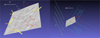Fig. 1 Schematic illustration of the hydrodynamic (left panel) and magnetic (right panel) drag on a moving light sail in a turbulent ISM with a magnetic field, B (green). The tumbling sail is represented by a thin gray sheet with a bumpy surface and a spin axis in the Z direction that precesses around its angular momentum, J, axis. The bombardment of atoms (with open and solid yellow dots representing pre- and post-collision trajectories) and photons (wavy arrows) leads to a force, Fgas (red), which can be decomposed into a drag, Fdrag, in the direction of the sail’s velocity, v (gray), and a sideways force, Fdrift. The induced currents (blue arrows) conducted away by surrounding charged particles lead to a Lorentz force, Fmag, with components perpendicular to both v and B.

2.2 Alfvén-wing drag by turbulent WNM

The ISM also contains magnetic fields with B ≈ 10 µG = 1 nT in the neutral medium and a few times larger in the molecular clouds (Draine 2011). As a light sail traverses the magnetic field with a relative velocity v_mag, an electric field v_mag×B is induced with a potential drop U ≃ 〈l〉v_magB across the time-averaged length, 〈l〉, of the tumbling light sail. An Alfvén wave is emitted along a wing (Drell et al. 1965), leading to a drag against v_mag with an acceleration

$$a_{\text{mag}}\simeq f_{\text{D}}{B}^2{v}_{\text{mag}}/2{\rho }_{\text{O}}{l}_3{\mu }_0{\overline{v}}_{\text{A}}$$(9)

in the direction (B · v_magB − |B|²v_mag)/|B|²|v_mag|, where f_D ≃ 〈l〉/l₁, with 1 ≳ f_D >> l₃/l₁, μ₀(= 4π × 10⁻⁷N A⁻²), $v_{\text{A}}=B/\sqrt{{\mu }_0{\rho }_g}$ is the Alfvèn speed, ${\overline{v}}_{\text{A}}={\mu }_0{v}_{\text{A}}\sqrt{1+M_{\text{A}}^2+2M_{\text{A}}\cos \gamma }~10-26\text{\hspace{0.17em}km\hspace{0.17em}}{\text{s}}^{-1}$ in the diffuse ISM, M_A = v_mag/v_A is the magnetic Mach number, and the angle cos γ = v_mag · B/(|v_mag| · |B|). When the rate of energy dissipation per unit mass in the Alfvén wing,

$${\dot{e}}_{\text{mag}}\simeq f_{\text{D}}{l}_1^2{v}_{\text{mag}}^2{B}^2/{\mu }_0{\overline{v}}_{\text{A}}{m}_{\text{O}},$$(10)

is balanced by ${\dot{e}}_{\text{gain}}\simeq v_{\text{d}}^2/2{\tau }_{*}$, a terminal speed is established with

$$\begin{array}{lll}{v}_{\text{term,mag}}\hfill & \simeq \hfill & {\left(\frac{{\rho }_{\text{O}}{l}_3{\mu }_0{\overline{v}}_{\text{A}}}{2f_D{B}^2{\tau }_{*}}\right)}^{1/2}{v}_{\text{d}}\hfill \\ \hfill & ~\hfill & 7.4{\left(\frac{l_3/f_{\text{D}}}{{10}^{-3}\text{m}}\frac{{\rho }_{\text{O}}}{{10}^3\text{\hspace{0.17em}kg\hspace{0.17em}}{\text{m}}^{-3}}\frac{{\overline{v}}_{\text{A}}}{10\text{\hspace{0.17em}km\hspace{0.17em}}{\text{s}}^{-1}}\right)}^{1/2}\left(\frac{1\text{\hspace{0.17em}\hspace{0.17em}nT}}{B}\right)\text{\hspace{0.17em}km\hspace{0.17em}}{\text{s}}^{-1}\hfill \end{array}$$(11)

which ~v_O with f_D ~ O(1) The timescale to reach v_terrm,mag is

$$\begin{array}{lll}{\tau }_{\text{term,mag}}\hfill & \simeq \hfill & \frac{{\rho }_{\text{O}}{l}_3{\mu }_0{\overline{v}}_{\text{A}}}{2f_D{B}^2}\hfill \\ \hfill & ~\hfill & 0.55\left(\frac{l_3/f_{\text{D}}}{{10}^{-3}\text{m}}\frac{{\rho }_{\text{O}}}{{10}^3\text{\hspace{0.17em}kg\hspace{0.17em}}{\text{m}}^{-3}}\frac{{\overline{v}}_{\text{A}}}{10\text{\hspace{0.17em}km\hspace{0.17em}}{\text{s}}^{-1}}\right){\left(\frac{1\text{\hspace{0.17em}\hspace{0.17em}nT}}{B}\right)}^2\text{\hspace{0.17em}Gyr}\hfill \end{array}$$(12)

over a travel distance

$$L_{\text{term,mag}}~{\tau }_{\text{term,mag}}{v}_{\text{term,mag}}\gtrsim 4\text{\hspace{0.17em}kpc.}$$(13)

Based on the same assumption that the light sail has preserved its original course, we only considered the limit L ≤ L_term,mag and v ≃ v_O.

The magnetic fields in the diffuse ISM are characterized by chaotic structure, although they are more orderly in star-forming GMCs (Crutcher 2012). We assume they are coupled to the large eddies in the WNM, which has a turbulent speed v_tur ~ (L_tur/pc)^0.38 km s⁻¹ that persists on the timescale (Choudhuri & Roy 2019)

$${\tau }_{\text{tur}}=L_{\text{tur}}/v_{\text{tur}}~{\left(L_{\text{tur}}/\text{pc}\right)}^{0.62}\text{Myr\hspace{0.17em}<<}{\tau }_{\text{term,mag}}$$(14)

on size scale 10⁻²pc ≲ L_tur ≲ 10²pc. The orientation between ‘Oumuamua v_mag and the background B (or equivalently γ) evolves on its travel timescale across eddies on scales with measured turbulent fields (L_tur ≲ 1 pc), τ_tur ~ L_tur/v_O ~ 0.1 Myr. This revision leads to greater variations, over a shorter timescale but on the same turbulent-eddy length scale, in the direction of the drag force on ‘Oumuamua than those due to the limited modification in the amplitude v_mag (Eq. (9) and Fig. 1).

For the spacecraft hypothesis, the initial value of v is preserved (~v_O) over a travel distance L ≤ L_term,mag. Over a brief travel time interval, t < τ_tur, the direction and magnitude of the drag by the turbulent fields on the light sail is sustained such that a_dnft ≃ a_mag and dispersion velocity σ_drift ≃ a_magt. Over a longer duration with τ_tur ≤ t ≤ τ_term,mag, the light sail encounters a new turbulent eddy with different v_tur, γ, and L_tur. While the magnitude of its a_drift ~ a_mag, random walk in the direction of relative motion leads to accumulative σ_drift ≃ (t/τ_tur)^1/2α_magτ_tur. The expected values of the deviation from the light sail’s initial course for these two limiting timescales are

$$E\left(d_{\text{mag}}\right)=\{\begin{array}{ll}{a}_{\text{mag}}{t}^2/2,\hfill & t<{\tau }_{\text{tur}}\hfill \\ {\left(t/{\tau }_{\text{tur}}\right)}^{3/2}{a}_{\text{mag}}{\tau }_{\text{tur}}^2/2,\hfill & t⩾{\tau }_{\text{tur}}\hfill \end{array}.$$(15)

Since the magnitude of v_tur and τ_tur are increasing functions of L_tur, that of a_mag and E(d_mag) also increases with L_tur (Eqs. (9) and (15)). In the present context, we estimated a lower limit for E(d_mag) by assuming the small L_tur ≤ 1 pc, where turbulent fields can be resolved. We also neglected the L_tur dependence in B.

The total trajectory deflection has an expected value $E\left(d_{\text{ISM}}\right)=\sqrt{E\left(d_{\text{gas}}^2\right)+E\left(d_{\text{mag}}^2\right)}$ with a Rayleigh distribution (see Eq. (C.6)). In the diffuse WNM, E(d_gas) < E(d_mag), τ_tur ~ 0.1 Myr such that E(d_ISM) ~ E(d_mag) and the light sail’s sideways motion undergo Levy walk over a travel length scale L ≳ 1 pc. In more dense CNM, E(d_ISM) ~ E(d_gas) ~ E(d_mag), τ_rot ~ 0.1 Myr and the sideways drift also follows a Levy walk path over travel length scale L ≳ 1 pc. Although E(d_ISM) ~ E(d_gas) > E(d_mag) in relatively dense (n_ISM > 10¹⁰ cm⁻³) GMCs, their hydrodynamic drag may lead to limited drift, despite their short τ_rot and τ_term,gas, due to their sparse volume filling factor.

In the evaluation of a_mag, we neglected the light sail’s spin because v_O >> 2πl₁/P. Nevertheless, this motion also leads to the excitation of Alfvén waves at both ends and dissipation of its spin energy E_rot = Iω²/2 (Zhang & Lin 2020) with a power

$$P_{\text{rot}}=\frac{B^2{\omega }^2{l}_1^4{\sin }^2\gamma }{4{\mu }_0{v}_{\text{A}}}.$$(16)

The damping timescale of rotation is

$${\tau }_{\text{rot,mag}}=\frac{E_{\text{rot}}}{P_{\text{rot}}}=\frac{{\rho }_{\text{O}}{l}_3{\mu }_0{v}_{\text{A}}}{B^2{\sin }^2ϵ}~20\left(\frac{{\rho }_{\text{O}}{l}_3}{1\text{\hspace{0.17em}kg\hspace{0.17em}}{\text{m}}^{-2}}\right)\text{Myr}$$(17)

if the Alfvén speed is assumed to be 1 kms^-1 in interstellar space. We see that this damping timescale is much longer than that due to the ISM’s ram pressure, τ_rot (Eq. (B.2)), and eddy turnover timescale, τ_tur. In the determination of relative velocity between it and the magnetic field, the light sail’s rotational damping due to magnetic torque can be neglected. Overall, we show that the rotational evolution timescale is inversely proportional to the gas number density and τ_tur ≈ 0.1 τ_rot ≈ 0.1 Myr for n_ISM ~ 10⁶m⁻³. The deflections induced by the magnetic field and the gas pressure are comparable (E(d_mag) ≈ E(d_gas)).

Under the assumption that a light sail’s original v is preserved before it enters the Solar System, there is no a priori reason for its v to be correlated with its l₁ or l₂. In contrast, the distance traveled, L, by freely floating interstellar asteroids and comets (with l₃ not much smaller than l₁ or l₂) is likely to be greater than min(L_term,gas, L_term,mag), and as such their motion will be gravitationally accelerated, dragged by the interstellar gas, and retarded by the interstellar magnetic field through Alfvén-wing drag (Zhang & Lin 2020). When a dynamical equilibrium is established by the balance of these effects, the ISOs attain a terminal speed relative to the LSR, v_d(l₁) ≃ min(v_term,gas, v_term,mag), which depends on their sizes.

3 Dynamics of a tumbling light sail in the Solar System

3.1 Sideways radiation force

During its sojourn through the Solar System, ‘Oumuamua endures intense heating near its perihelion. The surface temperature of the light sail increases rapidly, resulting in an increased average atomic kinetic energy of material. The atoms oscillate with anharmonic potentials in greater amplitudes, and therefore the material tends to expand with a larger separation between atoms. The fractional change in the light sail’s surface area can be estimated as ∆S/S = α_A∆T × 100%, where α_A is the thermal expansion coefficient. Molaro et al. (2020) estimate α_A = 8 × 10⁻⁶ for boulders and α_A = 2.4 × 10⁻⁴ for regolith. The thermal expansion coefficient, α, changes over the temperature as

$$\text{Δ}{\alpha }_{\text{A}}\approx 4\times {10}^{-9}\Delta T.$$(18)

The thermal equilibrium temperature at p_O is ~800 K, so the thermal expansion coefficient, α, is nearly constant. The expansion ratio of the area is ∆S/S ≈ 16% for regolith material and ∆S/S ≈ 0.6% for boulder material. Such thermal stress would not significantly alter the shape or surface roughness of the light sail.

However, the solar radiation pressure exerts a sideways force on ‘Oumuamua analogous to that due to ram-pressure drag (Fig. 1). When photons hit the surface, some are reflected immediately while some get absorbed and reradiated with a time lag. The latter effect is negligible since the thickness we consider here is so thin that it could be smaller than the penetration depth of the thermal wave, which leads to a nearly equal temperature all over the surface. The immediately reflected photons cause a recoil force F ≃ ΦA/c in the direction perpendicular to the surface. Reflection on its rough surface also leads to a torque T_rad (Eq. (A.3)), which cause ‘Oumuamua’s spin period, P_O, and orientation to evolve on a timescale τ_rad >> P_O (Eq. (A.4)).

The direction of this mean radiative force (integrated over a precession period) is about the wobble angle, θ, of ‘Oumuamua and the angle between the incident light and ‘Oumuamua’s angular momentum, θ. The heliocentric radial and sideways forces (in the antisolar and transverse directions) are

$$F_{\text{mean,r}}=\left(F_{\text{mean}}·e_r\right)e_r$$(19)

$$F_{\text{mean,s}}=F_{\text{mean}}-F_{\text{mean,r}}.$$(20)

The deflection angle of the force can be defined as

$$\alpha =\arccos \left(\frac{F_{\text{mean,r}}}{F_{\text{mean}}}\right).$$(21)

The values of the angle, α, for different θ and θ′ are shown in Fig. 8. In the trajectory of ‘Oumuamua, the value of θ′ varies. Since information on ‘Oumuamua’s spin (e.g., the directions of its spin angular momentum vector, principle axis, and precession angle) is not available, we used the mean value of α as an approximation. The mean value is α ≈ 26°, which gives the ratio of the sideways force to the radial force

$$\frac{F_{\text{mean,s}}}{F_{\text{mean,r}}}=\tan \overline{\alpha }\approx \frac{1}{2}.$$(22)

We can simply use this value to estimate the sideways deflection of ‘Oumuamua’s orbital paths through the Solar System.

Since the position of ‘Oumuamua is poorly constrained, we applied a Monte Carlo simulation to ‘Oumuamua’s orbital evolution over 80 days by testing 10⁵ cases with random initial orientations of angular momentum. Since the observation timescale of de-spin is ~24 days, we reset the angular momentum to a random orientation every 24 days. For each case, we calculated the mean ratio of the sideways force to the radial force along the way. The sideways force will lead to a displacement that is normal to the Keplerian orbital plane. The comparison of the result of the light sail and ‘Oumuamua is shown in Sect. 4.3.

In addition, the nongravitational model that fits the observation data best indicates that the radial force is A₁r⁻², with A₁ being constant. However, the tumbling motion of the light sail also leads to a variation in the magnitude of the force due to the time-varying orientation of the thin sheet. The timescale of the de-spin is ~24 days, which results in considerable changes in the angular momentum vector. We have already shown that the radiation force relies on the angular momentum (Eq. (D.11)), so we would expect a large variation range of the radiation force during 80 days of observation instead of a constant coefficient A₁. At the very least, even if the angular momentum does not change a lot during the orbit, the light angle (θ′) changes due to the orbital motion, which also leads to a time-varying radiative radial force. During the observational period (80 days), the mean-ratio changes of the radial force, ∆A₁/A₁, estimated from 10⁴ randomly generated test particles, show a normal distribution. The standard deviation is ~0.3, which indicates that the coefficient of the nongravitational force is expected to fluctuate by ~30%, while its reported value of A₁ = 4.92 ± 0.16 × 10⁻⁶ m/s² is inferred (Micheli et al. 2018) under the assumption of no change (i.e., ∆A₁ = 0).

Since the light curve and the radiation force components highly depend on the orientation of the light sail, they build a correlation with each other that can be examined for ISOs in the future. The correlation can be described quantitatively by the circular cross-correlation function:

$$R_{H,a}\left(\tau \right)=\frac{{\displaystyle {\sum }_{i=0}^{N-1}{H^{\prime }}_i{a^{\prime }}_{I+\tau }}}{{\left({\displaystyle {\sum }_{i=0}^{N-1}{H^{\prime }}_i^2}\right)}^{1/2}{\left({\displaystyle {\sum }_{i=0}^{N-1}{a^{\prime }}_i^2}\right)}^{1/2}},$$(23)

where ${H^{\prime }}_i$ and ${a^{\prime }}_{I+\tau }$ are the ith and (i + τ)th elements in the time-sequence absolute magnitude signal, H′, and the acceleration, a′, during a rotation cycle, which is centralized by

$$H^{\prime }=H-\overline{H},$$(24)

$$a^{\prime }=a-\overline{a}.$$(25)

Here, H and ā are the mean values of H and a. Considering the periodicity of the light curve and the radiation force, we made a periodic extension of H′ and a′, which leads to a modified correlation function:

$${R^{\prime }}_{H,a}\left(\tau \right)=\frac{{\displaystyle {\sum }_{i=0}^{N-1}{H^{\prime }}_i{a^{\prime }}_{\mathrm{mod}\left(\text{i}+\tau ,N\right)}}}{{\left({\displaystyle {\sum }_{i=0}^{N-1}{H^{\prime }}_i^2}\right)}^{1/2}{\left({\displaystyle {\sum }_{i=0}^{N-1}{a^{\prime }}_i^2}\right)}^{1/2}}.$$(26)

Therefore, the correlation function is a periodic function with the same period as H′ and a′ and we only need to pay attention to its behavior in one period. The correlation function reveals the similarity of the two signals at a time delay τ. The value range of R′_H,a(τ) is [−1, 1], and a larger value of |R′_H,a(τ)| implies a higher correlation between H and a.

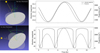Fig. 2 Illustration of the light sails in the one-facet illumination state and two-facet illumination (left panels) and their light curves (right panels). The rotation angular momentum is J, and the spin vector is along the major principal axis, z. The position vector r is pointing ‘Oumuamua away from the Sun. The solid lines denote the absolute magnitude, while the dashed line denotes the areas of projection along the sunlight direction. The imperfect consistency results from the nonzero phase angle ~20° (Fraser et al. 2018).

3.2 Light curve and visibility

The light curve of a tumbling light sail can exhibit a very large amplitude due to the large dimensional ratio. For a light sail with three axes of 60 m × 60 m × 0.3 mm, the amplitude could reach as large as 2.5 log (60 m/0.3 mm) ~ 13.25 in the case that the phase angle of the light sail is equal to 0°, which means the light sail is on the opposite side of the Sun relative to Earth. With a nonzero phase angle, the amplitude is even larger (Fraser et al. 2018). We used a symmetric ellipsoid (l₁ = l₂) model with an an isotropic-scattering surface for the calculation of the absolute magnitude of the light sail. The absolute magnitude is expressed as (Mashchenko 2019; Muinonen & Lumme 2015)

$$\begin{array}{lll}H\hfill & =\text{Δ}V-2.5\log {l^{\prime }}_3\frac{T_{\oplus }{T}_{\odot }}{T}-2.5\log [\cos \left({\lambda }^{\prime }-{\alpha }^{\prime }\right)\hfill & \hfill \\ \hfill & +\cos {\lambda }^{\prime }+\sin {\lambda }^{\prime }\sin \left({\lambda }^{\prime }-{\alpha }^{\prime }\right)\ln \left(\cot \frac{{\lambda }^{\prime }}{2}\cot \frac{1}{2}\left({\alpha }^{\prime }-{\lambda }^{\prime }\right)\right)],\hfill & \hfill \end{array}$$(27)

where

$$T_{\odot }=\left(S_1,S_2,S_3/{l^{\prime }}_3,\right),$$(28)

$$T_{\oplus }=\left(E_1,E_2,E_3/{l^{\prime }}_3\right),$$(29)

$$T=T_{\odot }+T_{\oplus }.$$(30)

Here S = (S₁, S₂, S₃) and E = (E₁, E₂, E₃) are the position vectors of the Sun and Earth in the corotating coordinate system. The parameter l′₃ is defined as l′₃ = l₃/l₁. The angle α′ is the angle between T_⊙ and T_⊕, and λ′ is the angle between T_⊙ and T. The parameter ∆V is the offset between the model and the observed light curve.

As already mentioned, the light curve can show an extremely large amplitude, which is shown in Fig. 2. Whether the amplitude is exotically large depends on the rotation state of the light sail and its orientation to the Sun, which can be categorized into two types. The first is the one-facet illumination state (OIS), where the light sail is in such a rotation that only one facet is exposed to sunlight. In this case, the projected area of the sunlight direction cannot reach the minimum value (l₁ × l₃) except when the sunlight comes from the edge of the light sail. Therefore, in the OIS the amplitude is usually not exotically large.

The second is the two-facet illumination state (TIS), where two facets of the light sail are successively exposed to sunlight due to rotation. In this case, the projected area of the sunlight direction reaches the lowest point the moment when the illuminated facet transfers from one to the other. In the TIS, the light curve of the light sail exhibits an extremely large amplitude, and the light sail becomes invisible for some time in its rotational cycle.

Figure 2 shows two examples of the light curve of the light sail, one for the OIS and the other for the TIS. Due to the symmetry of the square light sail, the periodical variation in the orientation of the light sail can be described by one parameter, the wobble angle (θ), as Fig. 2 shows. Another variable that affects the light curve is the direction of the position vector of the light sail relative to the Sun, which is equally translated to the illumination angle, θ′. The light sail is in the OIS when θ′ + θ ≤ 90° and is otherwise in the TIS.

Figure 3 shows the amplitude ∆H maps over a (θ, θ′) parameter space for the oblate shape, the prolate shape, and the light sail. We can see a clear boundary between the OIS and the TIS of the light sail in the amplitude map, although it does not strictly follows θ′ + θ ≤ 90° due to the nonzero phase angle.

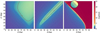Fig. 3 Amplitude map for the light curves of an oblate shape (left), prolate shape (middle), and light sail (right). The fractions of area where the amplitude ∆H is between 2.5 and 3 are 0.34, 0.1, and 0.015 for the oblate shape, prolate shape, and light sail, respectively.

4 Comparison between a free-floating light sail and ‘Oumuamua

4.1 Probability of close perihelion passage and occurrence timescale

In Sects. 2.1 and 2.2, we model the dynamics of ‘Oumuamua as a free-floating light sail traveling through a turbulent magnetized ISM under the influences of gas and magnetic drags on an intended journey to the Solar System. Together, these drag forces lead to a deviation with a Rayleigh distribution around an expected value $E\left(d_{\text{ISM}}\right)\simeq \sqrt{E\left(d_{\text{gas}}^2\right)+E\left(d_{\text{mag}}^2\right)}$, which is equivalent to an impact parameter in the gravitational domain of the Sun. The corresponding expected value of the perihelion distance 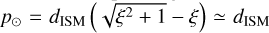$p_{\odot }=d_{\text{ISM}}\left(\sqrt{{\xi }^2+1}-\xi \right)\simeq d_{\text{ISM}}$, where ξ = GM/v²d_ISM << 1 and p_⊙ is generally much larger than ‘Oumuamua’s observed p_O (Fig. 4).

The probability of ‘Oumuamua attaining p_⊙ smaller than ‘Oumuamua’s observed perihelion p_O(0.26 au) is

$$P\left(p_{\odot }<p_{\text{O}}\right)=1-\exp \left(-\frac{p_{\text{O}}^2}{{\left(t/{\tau }_{\text{tur}}\right)}^3\text{Δ}{d}^2}\right),$$(31)

where $\text{Δ}d=a_{\text{ISM}}{t}_{\text{tur}}^2/2$. For various values of n_ISM, P(p_⊙ < p_O) is smaller than 10⁻³ over a travel distance L ≳ 1 pc, and it scales as P ∝ L⁻³ for larger L, which is shown in Fig. 4.

One possible solution for reconciling the low close-encounter probability with the expeditious discovery of ‘Oumuamua is the assumption that it was dispatched at one time with a population of N_tot cohorts, among which it had the smallest p_⊙. Based on the N_obs = 1 observation of ‘Oumuamua with p_O = 0.255 au, we infer N_tot = N_obs/P(p_⊙ < p_O) as a function of d. If they were launched concurrently at the same location, they would diffuse with a nearly uniform density $n=N_{\text{tot}}/d_{\text{ISM}}^3$ within a patch with a size ~d_ISM (Fig. 4). This dispersion would lead to a spread in the arrival time near the Sun τ_occurrence = 2d_ISM/v_O(n − 1), where n is the number per unit distance to the Sun (#/au) given by N_totp(d). Figure 5 shows that ‘Oumuamua-like objects would occur more frequently in the outer Solar System. A shorter distance for ‘Oumuamua’s birthplace leads to a shorter occurrence timescale. However, none of ‘Oumuamua’s hypothetical cohorts has been discovered yet, implying that ‘Oumuamua comes from a distant place where it has a much lower probability of reaching the Solar System (Fig. 4).

With its limiting sensitivity (24 magnitude), the Vera C. Rubin telescope can detect an ‘Oumuamua-like object out to ~1.6 au, and the number of cohorts passing through this distance is extrapolated to occur over time at intervals ∆τ_occur ~ 2–3 yr, which are insensitive to the distance they have traveled through the ISM (Fig. 5). The accumulated discoveries over the telescope’s first 10 yr of operation (Abell et al. 2009) correspond to a significant fraction of N(d ≤ 1.6 au) ~ 3–5 independent cohorts, from the same direction in interstellar space, which is smaller than that estimated for freely floating ISOs (~ 10)¹. Although this random drift may be rectified with a sophisticated guiding system, such a remote-control prowess during its arduous journey would be difficult to reconcile with ‘Oumuamua’s apparently freely tumbling motion, inferred from its evolving light curve (with P_O) and small sideways displacement, relative to that in the antisolar direction (Sect. 4.3) without introducing an additional assumption regarding an accidental guiding-system failure during its most recent Solar System passage.

4.2 Variability and visibility of ‘Oumuamua’s light curve

After an initial flurry of high-cadence observations (mostly provided by discretionary-time allocation), regular follow-up monitoring of ‘Oumuamua continued for another two months. Based on this limited data set, the following useful information can be extracted.

First, the amplitude of ‘Oumuamua’s light curve on October 25, 2017, from the Very Large Telescope (VLT) data is ∆H ~ 2.5 magnitudes, and the that on October 27,2017, from the Canada-France-Hawaii Telescope (CFHT) and the United Kingdom Infra-Red Telescope (UKIRT) data is ∆H ~ 3 magnitudes (Meech et al. 2017). The true amplitude could be larger due to the large error on the faintest point in the light curve, and thus it is safe to conclude that the amplitude was in range ∆H ≃ (2.5, 3) from October 25, 2017, to October 27, 2017.

Second, ‘Oumuamua is visible in later observations, from November 15, 2017, to January 2,2018, which means it is at least brighter than 27 magnitudes (Micheli et al. 2018).

Based on the above data, we investigated the probability of ‘Oumuamua being a light sail by considering the probabilities of the following two independent characteristics. (1) Regarding the variability, the light curve amplitude of ‘Oumuamua as a light sail is in the range ΔH ≃ (2.5, 3), based on the first fact. (2) Regarding the visibility, ‘Oumuamua as a light sail is brighter than 27 magnitudes and so is visible on each observational attempt, based on the second fact.

To calculate the probability of event A, we tested 10⁴ models, with the variable parameters wobble angle, θ, and the illumination angle, θ′, each sampled with 10² values uniformly distributed over (0◦, 90◦). Therefore, each of the 10⁴ models has an equal probability. Counting the number of models where the amplitude is in range ∆H ≃ (2.5,3) and dividing this number by 10⁴, we obtain the probability of event A. The likelihood function of the dimension ratio fi given event A is expressed as

$$L\left(f_l|\text{A}\right)=P_{fi}\left(\text{A}\right).$$(32)

Therefore, applying the maximum likelihood estimation (MLE), we find that the most likely shape of Oumuamua is the oblate shape with f_l = l₁/l₃ ~ 7. The results for other f_l are shown in the embedded panel in Fig. 6. We confirm that the probability of reproducing the observed variation amplitude (Mashchenko 2019) peaks at 10% with a 1:1:7 prolate axis ratio; at 34% with a 7:7:1 oblate axis ratio; and is ≲ 1.5% with a 1:1:5 × 10⁻⁶ thin-solar-sail axis ratio. This indicates that the most likely shape of Oumuamua is an oblate shape with an axis ratio of 7:7:1. Early studies favor a prolate shape according to the estimation of the density (Meech et al. 2017; Drahus et al. 2018), while Belton et al. (2018) suggest an oblate shape in the case that ‘Oumuamua’s rotational state is close to its highest energy state. By computing the possibilities of the best fitting prolate and oblate shape models, Mashchenko (2019) proposes that Oumuamua is more like an oblate spheroid with some torque exerted. Here our result supports the argument that Oumuamua is more likely to be oblate, making use of a different method, which compares the possibilities of various shapes inducing the observed amplitude of the light curve. This low probability of a light sail (~1.5%) is due to the common occurrence of a TIS, expected for thin freely tumbling light sails, which leads to very low surface exposure and reflection when they are nearly edge-on in the direction of the Sun (see Sect. 3.2), analogous to Saturn’s ring-plane crossing. In contrast, the tumbling motion in an OIS generally does not produce sufficiently large-amplitude modulations except under some special circumstances: θ + θ’′~ π/2, where θ and θ′ are the angles between the rotation axis relative to the normal vector of the light sail and to the direction of the Sun, respectively.

For event B, we generated 10⁴ test light sails with initial amplitudes in the range (2.5, 3) and added random torques with the magnitude given by Eq. (A.4) and a random direction. The magnitude of the torque decreases with the distance from the Sun, and the direction is assumed constant in the corotating reference frame over time. With a lack of information about the torque, we made the assumption of a constant torque in the corotating frame as previous work obtained a good fit to the light curve by applying this assumption (Mashchenko 2019). Due to the torque, the light sail can switch from the OIS to the TIS and therefore become invisible for part of its rotation cycle. For each model, we ran a 70-day simulation, covering from October 25, 2017 January 2, 2018. Since the timescale of spin evolution due to the torque is ~24 days, the rotation state of ‘Oumuamua since November 15, 2017, is considered to be random and uncorrelated to that on October 25, 2017, when the light curve is derived. We can thus calculate the visible fraction for each case and obtain the distribution of the whole sample set, which contains 10⁴ test particles. We deduce an expectation probability of 86.1 ± 3.2% of the entire 49-day monitoring interval that a freely tumbling light sail’s brightness is above the detection threshold (i.e., brighter than 27 magnitude), assuming a uniform sampling (gray distribution in Fig. 6). If the sampling is taken at epochs when ground-based and Hubble Space Telescope (HST) astrometry was obtained, the probability would be 84.8 ± 6.1% (blue distribution in Fig. 6).

The likelihood of the ISO as a light sail is revealed by comparing the distribution of the visible fraction of the tested 10⁴ cases with that purely inferred from observations between November 15, 2017, and to January 2, 2018 (49 days). The latter can be derived by statistic methods. For the simplest guess, one could use the MLE, which yields a ${\widehat{\text{Θ}}}_{\text{MLE}}=55/55=100\%$ probability of visibility. However, such an estimation only generates a single fixed value. To calculate the posterior probability distribution f(Θ|B) – that is, the probability distribution function of ‘Oumuamua’s being visible given the fact that it was successfully detected in all 55 observations (event B) – we refer to Bayesian inference for a continuous probability variable Θ ∈ [0, 1]:

$$f\left(\text{Θ|}B\left(n,k\right)\right)=\frac{f\left(B|\text{Θ}\right)f\left(\text{Θ}\right)}{{\displaystyle {\int }_0^{1}f\left(B|\text{Θ}\right)f\left(\text{Θ}\right)\text{dΘ}}},$$(33)

where B(n, k) is a statistical model describing a particular event of k times positive results out of n independent tests, and here we have n = k = 55 for event B. The f(Θ) is the prior probability distribution. Since we have no prior knowledge of ‘Oumuamua’s visible probability, it is reasonable to assume f(Θ) = 1; in other words, any visible probability, Θ, is equally likely. The f(B|Θ) is the probability of B(n, k) when the probability parameter Θ is given, and it can be written as

$$f\left(B\left(n,k\right)|\text{Θ}\right)={\text{Θ}}^k{\left(1-\text{Θ}\right)}^{n-k}.$$(34)

Thus, we can calculate the posterior probability distribution using

$$f\left(\text{Θ}|B\left(n,k\right)\right)=\frac{\left(n+1\right)!}{k!\left(n-k\right)!}{\text{Θ}}^k{\left(1-\text{Θ}\right)}^{n-k}.$$(35)

We show ‘Oumuamua’s posterior visible probability density distribution f(Θ|B(55,55) in Fig. 6. The expected a posteriori (EAP) of ‘Oumuamua’s visibility is

$$\begin{array}{lll}{\widehat{\text{Θ}}}_{\text{EAP}}=E\left(\text{Θ|}B\left(55,55\right)\right)\hfill & =\hfill & {\displaystyle {\int }_0^1\text{Θ}f\left(\text{Θ}|B\left(55,55\right)\right)\text{dΘ}}\hfill \\ \hfill & =\hfill & \frac{56}{57}\simeq 98.2\%.\hfill \end{array}$$(36)

This 3σ (or 2.2σ) discrepancy between the uniform (or nonuniform) sampling model and observational detection probability poses another challenge to the freely tumbling light-sail scenario. In fact, only 8 out of 10⁴ models report a 100% visible fraction.

The above analysis could be strengthened by additional observational results, such as the Minor Planet Center (MPC) astrometric database, after taking into account their limitations intrinsic to all photometric measurements obtained with astrometric purposes.

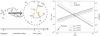Fig. 4 Schematic illustration of the diverse pathways of a constellation of Ntot tumbling solar sails traveling over a distance L through the turbulent magnetized ISM (left panel) and the expected value of the perihelion distance as a function of travel distance (right panel). As shown in the left panel, dispersive hydrodynamic and magnetic drag lead to a sideways drift, 4SM, and a dispersion in time of arrival, δt, at the Sun. The expected value E(dISM) (dashed gray circle) is generally much larger than the targeted Oumuamua’s perihelion distance, po. In the right panel, the expected value of the perihelion distance, E(p⊙) (solid lines), is shown as a consequence of deflection after traveling over a distance L through the ISM with a number density nISM. The probability of a single light sail striking the Solar System at a distance p⊙ ≤ pO (represented by a solid dot) from the Sun is shown with dashed lines.

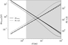Fig. 5 Fig. 5. Occurrence timescale (solid lines) and cumulative number (dashed lines) of ‘Oumuamua’s cohorts within d of the Sun for travel distances in the ISM L = 1 pc, 10 pc, 100 pc (increasing line widths). The timescale of occurrence of a light sail grows with increasing traveling distance, L, as a result of diffusion in the interstellar space. The timescale of occurrence within 100 au is insensitive to the travel distance, L, when L > 10 pc. The unshaded region is the observational domain of the first ∼10 yr of the Vera C. Rubin telescope.

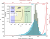Fig. 6 Fig. 6 – Histogram of 104 simulations of visible probability of a light sail versus posterior visible probability density distribution of Oumuamua over 49 days. The gray histogram represents the statistical result from a uniform random sampling, whereas the blue histogram is the statistical outcome from a nonuniform sampling that mimics ground-based and HST astrometry of Oumuamua. The dot-dashed gray and blue lines denote the mean values of these two statistical visibility simulations of a light sail, respectively. The dot-dashed and solid red lines represent the expected a posteriori estimation and the posterior probability distribution of Oumuamua’s visible probability (see Eq. (35)), respectively, based on the fact that Oumuamua was visible in all 55 observations. The embedded panel shows the likelihood that the amplitude of the light curve varies within the ranges ΔH ≃ (2.5,3) (Meech et al. 2017) and (2.5, 3.5) during the period October 25 = −27, 2017, for the light-sail, oblate shape, and prolate shape models.

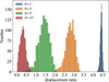Fig. 7 Distribution of the ratios of the sideways displacement to the radial displacement for different tumbling angles, θ, during observation (80 days). The initial rotation states of 103 test particles are constrained by the fact that the light curve amplitude is between 2.5 and 3. The sideways-to-radial displacement is 4.4 ± 0.1, 2.8 ± 0.2, 1.4 ± 0.3, and 0.3 ± 0.1 for the initial wobble angles θ ≤ Io, ≤ 3°, ≤ 5°, and ≤ 10°, respectively.

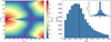Fig. 8 Fig. 8 – Ratio of the sideways radiation force (Fmean,s) to the radial radiation force (Fmean,r) for a tumbling light sail suffering radiation pressure. (a) Distribution of the deflection angle, α, with tan α = Fmean,s/Fmean,r for the whole value range of the wobble angle, θ, and the photon incident angle, θ′. (b) Distribution of Fmean,s/Fmean,r for 105 light sails with random θ and θ′ after an 80-day motion. The mean value of the sideways-to-radial force ratio is 0.7 ± 0.4 for light sails, while this ratio for Oumuamua is ~0.08 (Micheli et al. 2018), which is a discrepancy (Micheli et al. 2018) of ~1.5σ. The embedded panel shows the distribution of ∆A1/A1 for 104 generated pseudo ‘Oumuamuas during 80-day movements, where A1 and ΔA1 denote the coefficient of the radiation pressure and its variation over 55 days, from November 15, 2017, to January 2, 2018 (see Sect. 3). The standard deviation, denoted by the dash lines, is 0.3.

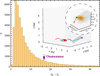Fig. 9 Fig. 9 – Histogram of the ratio between the parallel deviation and the normal deviation. The radiation-pressure-induced deviation from a Keplerian trajectory during Oumuamua’s sojourns through the inner Solar System are shown with the dashed green line. The red star represents the Sun, and solid black, cyan, blue, and red arcs indicate the orbits of Mercury, Venus, Earth, and Mars, respectively. The purple cross indicates the position of Oumuamua at the last record. In total, 5 × 104 light-sail models with randomized initial spin orientations are integrated from Oumuamua’s discovery position for the same period of time. An additional Keplerian trajectory without radiation force is integrated, with which an orbital plane is defined. The circular inset panel zooms in to show Oumuamua’s last position (purple cross) surrounded by all light-sail models at the end of integration. And deviations from the Keplerian orbit (green square in the plane) are measured in the parallel and perpendicular directions to the orbital plane (indicated by two red arrows). The distribution of the ratio of the parallel displacement to the normal displacement peaks at ~3, while Oumuamua lies at ~17, which is obtained by applying the nongravitational acceleration suggested by Micheli et al. (2018).

Fig. 10 Light curve (upper panels), radiation acceleration (middle panels), and correlation within one day between them (bottom panels) for the light sail in the OIS (left panels) and in the TIS (right panels).

4.3 Displacement normal to the orbit plane

‘Oumuamua’s “persistently visible” magnitude may be maintained under a highly unlikely scenario, that its tumbling motion is marginally kept in a protracted OIS near its current (θ + θ′ ≃ π/2) configuration. This probability can be constrained by the observationally inferred nongravitational force and acceleration in the radial (F_r away from the Sun) and sideways (F_s orthogonal to the radial) directions, due to the reflective torque on the light sail s surface (Micheli et al. 2018). Figure 7 shows that for θ < 5° – 10°, ∆r_mean,s > ∆r_mean,r. For a randomly distributed value of θ, the most likely mean ratio of these components F_mean,s/F_mean,r ~ 0.7 ± 0.4 (Eq. (22), Figs. 8 and 9), while it is 0.08 for the observed trajectory of ‘Oumuamua (Micheli et al. 2018), deviating from the light-sail model by 1.5σ. Since these forces correlate with the light curve (Fig. 10), which evolves due to changes in ‘Oumuamua’s tumbling motion (P_O) and orbit, a ~30% revision in the radiation-pressure-driven acceleration is expected during its 80 days observational window. Observation data (Micheli et al. 2018) show that their ratio is only ~0.08, while in our simulation the fraction of the ratios equal to or smaller than 0.08 is only 2%.

As a result of the sideways force, an observable non-radial displacement is introduced to ‘Oumuamua’s trajectory. The sideways force causes a displacement normal to the orbital plane. The normal displacement is a good indication of the sideways force since the radial displacement and the transverse displacement are not well defined due to their changes of direction in the orbital motion. We used the REBOUND code (Rein & Liu 2012) and the REBOUNDx extension (Tamayo et al. 2019) to compute the ratio of the parallel displacement (in-plane displacement) to the normal displacement for 5 × 10⁴ randomly generated models. The distribution of the ratio is shown in Fig. 9. The peak of the ratio distribution is at ~3, implying that the most likely parallel-to-normal ratio is ~3 for the light sail. However, the parallel-displacement ratio of ‘Oumuamua was found to be ~17 by applying the nongravitational acceleration reported by Micheli et al. (2018). Although existing data do not have adequate accuracy to firmly establish any discriminating constraints on the light-sail hypothesis, they highlight the requirement of low-probability coincidences for ‘Oumuamua.

Since both the radiation force and the light curve highly depend on the orientation and rotation of the light sail, there is a strong correlation between the acceleration and light curve. Figure 10 shows an example of the correlation functions between the absolute magnitude, H′, and the radiation force, a′, for the light sail. The correlation functions exhibit a regular mode, and the maximum value reaches 0.4 for both OIS and TIS, implying a high correlation between the absolute magnitude and the radiation force. However, for tumbling comets with nongravitational acceleration due to outgassing, the correlation is expected to be much weaker due to the chaotic tumbling motion and thermal delay. This correlation for a light sail declines within several rotational cycles (~2 days), which is shown in Fig. 11; this allows us to place a requirement on the high-cadence observational data. Therefore, with help of a huge amount of highly accurate observation data in the future, we will be able to identify the light sail by investigating the correlation between the light curve and the force curve.

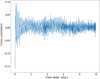Fig. 11 Correlation between the light curve and the acceleration as a function of the delay time for a light sail. The correlation declines quickly within two days, which indicates that high-cadence time series data are required for the diagnosis of a light sail.

5 Summary and discussions

We have analyzed the dynamics of light sails in the interstellar space and Solar System and show that their signatures, if they exist, are observable and can be quantitatively analyzed with some forthcoming instruments, such as the Vera C. Rubin telescope and the Chinese Space Station Telescope (CSST). In the forthcoming observations, our methods can function as a pipeline to test the probability of an ISO being a light sail.

After applying these analyses in the context of the first-discovered ISO ‘Oumuamua, we find its observed properties to be incompatible with those expected from the light-sail hypothesis. Based on inferences from ‘Oumuamua’s data, we suggest additional stringent tests for any potential interstellar light sails:

1. Freely floating light sails endure drifts due to the magnetic and gas drag by the ISM. The drift of freely rotating light sails in the ISM can reach ~100 au over a travel distance of 1 pc. It increases with the travel distance as ~L³. In order for any light sail to venture into ‘Oumuamua’s intended closest approach to the Sun, a constellation of light-sail probes is needed. Some members of this flotilla should be detectable over the next few years;

2. The solar radiation would cause a sideways pressure if the net flux of incident solar light is not parallel or antiparallel to the light sails orbital trajectories. Consequently, any tumbling motion would impose a non-negligible sideways radiation force on light sails and provoke sideways displacements. In reality, the sideways force experienced by ‘Oumuamua as inferred from its observed orbit is one order of magnitude smaller than the radial force, whereas these forces are expected to be comparable for a typical tumbling light sail. Quantitatively, the observed ‘Oumuamua ratio deviates from the value expected for a light sail by ~1.5 σ. Moreover, the probability distribution of the ratio between the displacement in the orbital plane to that in the normal direction for light sails peaks at 3, while the observationally inferred ratio is 17 for ‘Oumuamua. The displacement normal to the orbital plane is expected to be correlated with the light curve of light sails. This test can be applied with future high-cadence observations;

3. The amplitude of the light curve can also be used to assess the likelihood of the axis ratio of ISOs. Our analysis of ‘Oumuamua s observed light curve suggests it is most likely to have an oblate shape with an axis ratio of ~7:7: 1, while the probability for such a light curve to be due to a light sail is ~1.5%. The large amplitudes in the light-curve variation and the prospect of undetectable phases during their tumbling motion can be used to quantify the light-sail probability for future observations of ISOs. The probability for a light sail to be persistently brighter than the 27th magnitude in all 55 ‘Oumuamua s monitoring attempts during the two months after its discovery is estimated to be 0.4%. We find a 3σ discrepancy between ‘Oumuamua’s perfect-detection record and the expectation based on the light-sail hypothesis.

We suggest that ‘Oumuamua is unlikely to be a light sail. The dynamics of an intruding light sail would give rise to observational features such as the occurrence of its cohorts, a remarkable sideways radiation force and normal displacement from the Kepler orbit, a light curve with an extremely high amplitude, and irregular invisibility in the sky. These features can be quantitatively identified and analyzed with our methods in future surveys.

Acknowledgements

We thank Greg Laughlin and Scott Tremaine, as well as Tingtao Zhou, Patrick Michel, Meng Su, Xiaojia Zhang, Wenchao Wang, Yue Wang, Quanzhi Ye, Shoucun Hu, and Bo Ma for useful discussions. This work is supported by the National Natural Science Foundation of China under grant No. 11903089, the Guangdong Basic and Applied Basic Research Foundation under grant Nos. 2021B1515020090 and 2019B030302001, the Fundamental Research Funds for the Central Universities, Sun Yat-sen University under grant No. 22lgqb33, and the China Manned Space Project under grant nos. CMS-CSST-2021-A11 and CMS-CSST-2021-B09.

Appendix A ISM’s torque on the light sail’s asymmetric surface and ‘Oumuamua’s spin

The large-amplitude variations in ‘Oumuamua’s light curve suggest it has an asymmetry surface. Such a feature may be inherent in its original architecture, be bestowed by micro-meteorite and cosmic-ray bombardments during its passage through the ISM, or be deformed by the thermal stress due to a nonuniform albedo. Although the light sail may also have encountered an air mass comparable to m_O after traveling L ≳ L_term,gas (Bialy & Loeb 2018), the ISM’s condensation on its surface is unlikely to significantly modify its thickness, l₃, especially in the limit L ≲ L_term,gas.

With an asymmetric shape, the light sail endures a torque due to the gas ram pressure and dust bombardment. Over time, this torque changes the light sail’s spin orientation and frequency (Zhou 2020). We approximate the torque due to gas pressure by

$$T_{\text{gas}}\simeq C_{z,\text{ISM}}{m}_{\text{p}}{n}_{\text{ISM}}{v}^2{l}_1^3,$$(A.1)

where C_z,ISM measures the efficiency of the gas torque, depending on light sail’s shape and surface topology. Similarly, torque due to dust bombardment (Stern 1986) is

$$T_{\text{dust}}\simeq C_{z,\text{ISM}}{\overline{\mu }}_{\text{gr}}\left(h_1+h_2\right)v{v}_{\text{ej}}{l}_1^3,$$(A.2)

where μ_gr is the mean mass density of the interstellar grains, h₁ and h₂ are the ratios of evaporated mass and the ejected mass of the object to the mass of incident grain, respectively, and v_ej is the velocity of the ejection. The dust torque, T_dust, does not make much difference unless ‘Oumuamua moves very fast (e.g., > 20 km/s).

In order to infer the magnitude of C_z,ISM, we note that the irregular roughness and/or curvatures on the light sail’s surface also lead to a finite radiative torque, and the torque coefficient C_z,ISM ≃ C_z,rad (Zhou 2020). The finite magnitude of the radiative torque arises from a residual radiation pressure exerted by the incident photons on an asymmetric surface that does not cancel out during any spin period (Rubincam 2000; Vokrouhlicky & Capek 2002; Bottke Jr et al. 2006). Averaged over time, the radiative torque is approximately

$$T_{\text{rad}}~\frac{C_{z,\text{ra}d}\text{Φ}A{l}_1}{c},$$(A.3)

where the efficiency of the radiative torque C_z,rad ≃ C_z,ISM, c is the light speed, A = f_Al₁l₂, and Φ = L_⊙/4πr² is the solar flux at the object’s heliocentric distance, r. Subject to this torque, the light sails spin to evolve on a timescale

$$T_{\text{rad}}\simeq \frac{\omega I_3}{T_{\text{rad}}}\simeq \frac{\omega {\rho }_{\text{O}}{l}_1{l}_{3}c}{8C_{z,\text{rad}}\text{Φ}{f}_{\text{A}}},$$(A.4)

where its moment of inertia $I_3~{\rho }_{\text{O}}{l}_1^3{l}_2{l}_3$.

‘Oumuamua’s observed de-spin timescale (P_O/P_O ~ 24 days) during its passage through the inner Solar System has been explained in terms of this radiative torque (Mashchenko 2019). Applying our model parameters to Eq. (A.4), we infer C_z,rad (as well as C_z,ISM) ~ 4 × 10⁻⁴. From this value of both C_z,rad and C_z,ISM, we place constraints on the surface roughness of the light sail with a set of Monte Carlo simulations. For our numerical model of the light sail shape, we constructed hundreds of surfaces with ~1500 vertexes and ~3000 facets in each generated surface (as shown in Fig. 1). The roughness can be measured by the standard deviation of departures, ∆h, from vertexes to a hypothetical perfectly flat sheet. We tested different cases where the deviations are ∆h ≃ (0.1,1,10,10²)l₃. For each case, we processed 10000 runs with random surfaces and random orientations. Figure A.1 shows a typical example of the distribution of the departures of vertexes from the plane with the standard deviation of 50 mm. The results show that the surface cannot introduce a sufficiently large torque efficiency (C_z,ISM = 4 × 10⁻⁴) unless it has a roughness such that the deviation of the vertexes is hundreds of times greater than the light sail thickness (l₃ ~ 3–5 × 10⁻⁴m). The results are shown in Fig. A.1.

Appendix B Spin evolution during passage through the ISM

During its passage through the ISM with v ≤ 20 km s⁻¹, the light sail s spin evolution is mostly determined by the gas torque (Zhou 2020), T_gas (Eq. A.1). The maximum moment of inertia, $I\approx m{l}_1^2/8$, of a solar sail (with a large dimension ratio l1 /l3 >> 1) dominates over that of its command module with sizes ≲ 0.1l₁. (The actual integrated moment of inertia of the spacecraft is likely to be slightly smaller than this value since part of the mass is contained in the command module located near the center of the spacecraft.) The angular acceleration of the space craft is

$$\dot{\omega }\simeq \frac{T_{\text{gas}}}{I}=\frac{8C_{z,\text{ISM}}{m}_{\text{p}}{n}_{\text{ISM}}{v}^2}{{\rho }_{\text{O}}{l}_1^2}.$$(B.1)

The light sail s spin angular momentum and its direction of acceleration, a_gas, change on the timescale of

$${\tau }_{\text{rot}}\simeq \frac{\omega }{\dot{\omega }}~\frac{\omega {\rho }_{\text{O}}{l}_1{l}_3}{8C_{z,\text{ISM}}{m}_{\text{p}}{n}_{\text{ISM}}{v}^2}~\frac{\omega l_1{\tau }_{\text{term,gas}}}{8C_{z,\text{ISM}}v}.$$(B.2)

Since the coefficient of the gas torque, C_z,ISM, has the same order of magnitude of that of the radiative torque, C_z,rad (Zhou 2020), we estimate C_z,ISM ≃ C_z,rad ≃ 4 × 10⁻⁴ from ‘Oumuamua’s observed de-spin rate during its passage through the Solar System (Appendix A).

It is possible for the T_gas torque to spin down the light sail, deplete its spin angular momentum, and restart a subsequent rotational cycle with a different orientation. It is also possible for the torque to transfer positive angular momentum to the object until it reaches a breakup spin limit. A creative epilogue (Bialy & Loeb 2018; Loeb 2021) of the spacecraft hypothesis is the suggestion that ‘Oumuamua’s tumbling motion may have been intentionally instated to enable the spacecraft to emit and receive signals in and from all directions. Since any initial spin state can only be preserved over τ_rot ~ 1(ρ_Ol₃/1 kg m⁻²)(10⁶m⁻³/n_g)(l₁/60m)Myr, such an assumption would require that ‘Oumuamua s interstellar odyssey, with its observed v_O, be limited to a maximum traveled distance L_max ≈ 10 pc. The total population of stars, including white dwarfs and brown dwarfs, in this domain is ~400.

Appendix C Accumulative drift

In the limit t ≥ t_rot and t ≥ t_tur, E(d_gas) and E(d_mag) (in Eqs. 8 and 15) are derived for randomly evolving acceleration a_gas and a_mag. For the convenience of a general discussion, we use variables {E(d_rand), ∆t, a_rand} to represent both {E(d_gas), τ_rot, a_drflt) and {E(d_mag), τ_tur, a_mag}. The motion of the object follows Langevin’s equation:

$$\ddot{d}=-\lambda v+a_{\text{rand}},$$(C.1)

where the drag coefficient λ = 0 in our case. We started with the simplest 1D model, where the acceleration a_rand,i∙ is reset, after each time step ∆t, to be ±a_rand with a 50% probability for each value. The velocity gains a random increment a_rand time interval ∆t. The velocity at time t is the sum of the independent random variable a_rand,i∙ for i = 0,1, …N_rand with N_rand = t/∆t. According to the central limit theorem, the probability distribution of velocity, v_rand, obeys a Gaussian distribution: $N\left(0,N_{\text{rand}}{a}_{\text{rand}}^2\text{Δ}{t}^2\right)$. The displacement is

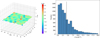Fig. A.1 Example of the rough surface with ∆h ~ 0.05 m (left panel) and the distribution of the values of Cz for 104 runs on random surfaces with ∆h ≈ 0.05 m. The mean value of Cz is (4 ± 4) × 10−4.

$$d_{\text{rand}}={\displaystyle {\int }_0^{\tau }vd\tau .}$$(C.2)

The distribution of drand can be solved by determining the distribution of the limit of the right-hand sums:

$$\begin{array}{ccc}{d}_{\text{rand}}={\displaystyle \sum _{i=0}^{N_{\text{rand}}-1}\left(v_i\text{Δ}t\right)}& \text{where}& v_i={\displaystyle \sum _{k=0}^{i-1}{a}_{\text{rand,k}}\text{Δ}t}.\end{array}$$(C.3)

Since only the acceleration is the independent variable, we needed to unfold Eq C.3 in terms of a_rand.i:

$$\begin{array}{lll}{d}_{\text{rand}}\hfill & =\hfill & \text{Δ}t\left(v_{\text{rand,0}}+v_{\text{rand,1}}+\dots +v_{N_{\text{rand}}-1}\right)\hfill \\ \hfill & =\hfill & \text{Δ}{t}^2[a_{\text{rand},0}+a_{\text{rand,1}}+\dots +a_{N_{\text{rand}}-2}\hfill \\ \hfill & \hfill & +\left(a_{\text{rand,0}}+a_{\text{rand,1}}+\dots +a_{N_{\text{rand}}-2}\right)]\hfill \\ \hfill & =\hfill & \text{Δ}{t}^2\left(N_{\text{rand}}-1\right)a_{\text{rand,0}}+\left(N_{\text{rand}}-2\right)a_{\text{rand,1}}+\dots +a_{N_{\text{rand}}-2}\hfill \\ \hfill & =\hfill & \Delta t^2{\displaystyle \sum _{i=0}^{N_{\text{rand}}-2}\left(N_{\text{rand}}-1-i\right)a_i}\hfill \end{array}.$$(C.4)

Due to the central limit theorem, the sum of independent random variables a_rand,i (with the variance of arand) exhibits a Gaussian distribution, with the variance

$$\begin{array}{lll}\text{Var}\left(d_{\text{rand}}\right)\hfill & =\hfill & \text{Var}\left({\displaystyle \sum _{i=0}^{N_{\text{rand}}-2}\left(N_{\text{rand}}-1-i\right)a_{\text{rand,}i}\text{Δ}{t}^2}\right)\hfill \\ \hfill & =\hfill & {\displaystyle \sum _{i=0}^{N_{\text{rand}}-2}{\left[\left(N_{\text{rand}}-1-i\right)a_{\text{rand}}\text{Δ}{t}^2)\right]}^2}\hfill \\ \hfill & =\hfill & a_{\text{rand}}^2\text{Δ}{t}^4\left[1+2^2+\dots +{\left(N_{\text{rand}}-1\right)}^2\right]\hfill \\ \hfill & \simeq \hfill & \frac{1}{3}{a}_{\text{rand}}^2\text{Δ}{t}^4{N}_{\text{rand}}^3\hfill \end{array}.$$(C.5)

Therefore, the displacement $d_{\text{rand}}~N\left(0,a_{\text{rand}}^2\text{Δ}{t}^4{N}_{\text{rand}}^3/3\right)$. The expected value $\text{E}\left(\left|d_{\text{rand}}\right|\right)~a_{\text{rand}}\text{Δ}{t}^2{N}_{\text{rand}}^{3/2}/\sqrt{3}$. The displacement in higher dimensions obeys a chi distribution. In particular in a 2D case, the probability distribution of the displacement, d, is given by a Rayleigh distribution:

$$p\left(d\right)=\frac{2d}{N_{\text{rand}}^3\text{Δ}{d}^2}\exp \left(-\frac{d^2}{N_{\text{rand}}^3\text{Δ}{d}^2}\right),$$(C.6)

with $\text{Δ}d=a_{\text{rand}}\text{Δ}{t}^2/\sqrt{3}$. This analytic approximation of p(d) was verified with a Monte Carlo simulation for the random-walk process (Fig. C.1). The expected value is expressed as

$$\text{E}\left(d_{\text{rand}}\right)=a_{\text{rand}}\text{Δ}{t}^2{N}_{\text{rand}}^{3/2}/\sqrt{6}=a_{\text{rand}}\text{Δ}{t}^{1/2}{t}^{3/2}/\sqrt{6}.$$(C.7)

Appendix D Radiation force for a tumbling light sail

D.1 Coordinate system

In order to reconstruct ‘Oumuamua’s equation of motion in the Solar System, we approximated it as an object with a non-principal axis rotation analogous to that of a symmetric top. In this case, the spin axis rotates around the angular momentum vector, J. At a heliocentric position, r, the force components along the direction r × J cancel each other out. The resulting net force by radiation pressure lies on the (r, J) plane. The mean force can be considered in a coordinate system described by three basis vectors, e_X, e_Y, and e_Z, with

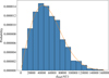Fig. C.1 Normalized distribution of dISM for 1000 test particles that feel a random magnetic force when the travel distance is 100 pc. The orange curve is the Rayleigh distribution given by Eq. C.6.

$$\{\begin{array}{l}{e}_Z=\frac{J}{J}\hfill \\ e_Y=\frac{e_Z\times r}{r}\hfill \\ e_X=e_Y\times e_Z.\hfill \end{array}$$(D.1)

Since ‘Oumuamua’s spin frequency, ω_O, is much faster than its heliocentric orbital angular frequency, we can approximate e_r to be a constant within a rotational period. We also need a rotating coordinate frame, described by the three unit vectors e_x, e_y, and e_z along the three principal axes of ‘Oumuamua. Here e_z points in the positive direction of the principal axis of the maximum moment of inertia. The orientation of the rotating coordinate frame can be described by three Euler angles, ϕ, θ, and ψ (in x − z − x sequence). For an arbitrary vector k, the transformation between the nonrotating reference frame (XYZ) and the rotating reference frame (xyz) is k = R(ϕ, θ, ψ)k′. Here k denotes the vector in the nonrotating reference frame while k′ denotes the vector in the rotating frame. Here R(ϕ, θ, ψ) is the rotation matrix.

In the spaceship hypothesis, ‘Oumuamua is considered as an extremely thin solar sail (Fig. 1). To simplify the problem, we made two main assumptions in this context. First, the radiation pressure mainly exerts on the maximum face, whose normal vector is along the z axis, and the forces felt by other faces are ignored. Second, we assume the extremely thin ‘Oumuamua is a near-symmetric top that has a moment of inertia I = (I₁, I₂, I₃) with I₁ = I₂ < I₃. Under the first assumption, the radiation pressure on the a perfectly reflecting light sail is

$$F_{\text{radiation}}=\frac{A{L}_{\odot }}{2\pi r^{2}c}\left|e_r·e_z\right|\left(e_r·e_z\right)e_z.$$(D.2)

Here A|e_r · e_z| is the face area that is normal to the solar light and L_⊙ is the solar luminosity. The unit vector e_z is

$$e_z=R\left(\varphi ,\theta ,\psi \right){e^{\prime }}_z=\left(\begin{array}{c}\sin \varphi \sin \theta \\ -\cos \varphi \sin \theta \\ \cos \theta .\end{array}\right).$$(D.3)

Without the loss of generality, we set the initial ϕ₀ = π/2 so that the initial e_z lies on the plane (X, Z) and e_z becomes

$$e_z=\left(\begin{array}{c}\sin \left({\varphi }_0+\varphi \right)\sin \theta \\ -\cos \left({\varphi }_0+\varphi \right)\sin \theta \\ \cos \theta \end{array}\right)=\left(\begin{array}{c}\cos \varphi \sin \theta \\ \sin \varphi \sin \theta \\ \cos \theta \end{array}\right),$$(D.4)

where θ is the nutation angle. The unit vector of the position in the nonrotating reference frame (XYZ) can be assigned as e_r = (sin θ′, 0, cos θ′), where θ′ is in the range (0, π). The solution for a symmetric top is

$$\begin{array}{ccc}\dot{\theta }=0,& \text{and}& \dot{\varphi }=\frac{J}{I_2}.\end{array}$$(D.5)

D.2 Averaging over a spin period

With a constant θ, F_radiation is a periodic force that is modulated on the timescale of the precession period 2π/ϕ. The mean force, integrating over its period, is

$$F_{\text{mean}}=\frac{1}{2\pi }{\displaystyle {\int }_0^{2\pi }{F}_{\text{radiation}}d\varphi }=\frac{1}{2\pi }{\displaystyle {\int }_0^{2\pi }\frac{A{L}_{\odot }}{2\pi r^{2}c}\left|e_r·e_z\right|\left(e_r·e_z\right)e_{z}d\varphi ,}$$(D.6)

where e_r · e_z = k₁ cos ϕ + k₂ = k₁(cos ϕ + k₂/k₁), where k₁ = sin θ sin θ′ and k₂ = cos θ cos θ′.

In the limit k₂/k₁ ≥ 1, equivalently θ′ ≤ π/2 − θ, we have e_r · e_z ≥ 0, and the mean force can be expressed as

$$F_{\text{mean}}=\frac{1}{2\pi }{\displaystyle {\int }_0^{2\pi }\frac{S{L}_{\odot }}{2\pi r^{2}c}{\left(e_r·e_z\right)}^2{e}_{z}d\varphi }$$(D.7)

$$=\frac{A{L}_{\odot }}{4{\pi }^2{r}^{2}c}{\displaystyle {\int }_0^{2\pi }{\left(k_1\cos \varphi +k_2\right)}^2\left(\begin{array}{c}\cos \varphi \sin \theta \\ \sin \varphi \sin \theta \\ \cos \theta \end{array}\right)d\varphi .}$$(D.8)

With a constant θ,

$$F_{\text{mean}}=\frac{A{L}_{\odot }}{4\pi r^{2}c}\left(\begin{array}{c}2k_1{k}_2\sin \theta \\ 0\\ k_1^2+2k_2^2.\end{array}\right).$$(D.9)

In the limit k₂/k₁ ≤ −1, or equivalently θ′ ≥ π/2 + θ, e_r · e_z ≤ 0, and the mean force reduces to

$$\begin{array}{lll}{F}_{\text{mean}}\hfill & =\hfill & -\frac{1}{2\pi }{\displaystyle {\int }_0^{2\pi }\frac{A{L}_{\odot }}{2\pi r^{2}c}{\left(e_r·e_z\right)}^2{e}_{z}d\varphi }\hfill \\ \hfill & =\hfill & -\frac{A{L}_{\odot }}{4{\pi }^2{r}^{2}c}\left(\begin{array}{c}2\pi k_1{k}_2\sin \theta \\ 0\\ \pi \left(k_1^2+k_2^2\right)\cos \theta .\end{array}\right)\hfill \end{array}$$(D.10)

In the intermediate region with −1 < k₂/k₁ < 1, or equivalently π/2 − θ < θ′ < π/2 + θ, we find that the condition for e_r · e_z > 0 is −β < ϕ < β where β is defined as $\beta =\arccos \left(-\frac{k_2}{k_1}\right)$. The mean force becomes

$$\begin{array}{l}{F}_{\text{mean}}=\frac{1}{2\pi }{\displaystyle {\int }_{-\beta }^{\beta }\frac{S{L}_{\odot }}{2\pi r^{2}c}{\left(e_r·e_z\right)}^2{e}_{z}d\varphi -\frac{1}{2\pi }{\displaystyle {\int }_{-\pi }^{-\beta }\frac{S{L}_{\odot }}{2\pi r^{2}c}{\left(e_r·e_z\right)}^2{e}_{z}d\varphi -}}\hfill \\ \frac{1}{2\pi }{\displaystyle {\int }_{\beta }^{\pi }\frac{S{L}_{\odot }}{2\pi r^{2}c}{\left(e_r·e_z\right)}^2{e}_{z}d\varphi }\hfill \\ =\frac{S{L}_{\odot }}{2{\pi }^2{r}^{2}c}{\displaystyle {\int }_0^{\beta }{\left(k_1\cos \varphi +k_2\right)}^2\left(\begin{array}{c}\cos \varphi \sin \theta \\ 0\\ \cos \theta \end{array}\right)d\varphi }\hfill \\ -\frac{S{L}_{\odot }}{2{\pi }^2{r}^{2}c}{\displaystyle {\int }_{\beta }^{\pi }{\left(k_1\cos \varphi +k_2\right)}^2\left(\begin{array}{c}\cos \varphi \sin \theta \\ 0\\ \cos \theta \end{array}\right)d\varphi }\hfill \\ =\frac{A{L}_{\odot }}{4{\pi }^2{r}^{2}c}\left(\begin{array}{c}{F}_1\left(\theta ,{\theta }^{\prime }\right)\\ 0\\ F_3\left(\theta ,{\theta }^{\prime }\right).\end{array}\right)\hfill \end{array}$$(D.11)

where

$$\begin{array}{lll}{F}_1\left(\theta ,{\theta }^{\prime }\right)\hfill & =\hfill & 2k_1^2\sin \theta \left(2\sin \beta -\frac{2}{3}{\sin }^3\beta \right)\hfill \\ \hfill & +\hfill & 4k_2^2\sin \theta \sin \beta +4k_1{k}_2\sin \theta \left(\beta +\sin \beta \cos \beta -\frac{\pi }{2}\right),\hfill \\ F_3\left(\theta ,{\theta }^{\prime }\right)\hfill & =\hfill & 2k_1^2\cos \theta \left(\beta +\sin \beta cos\beta -\frac{\pi }{2}\right)\hfill \\ \hfill & +\hfill & k_2^2\cos \theta \left(4\beta -2\pi \right)+8k_1{k}_2\cos \theta \sin \beta ).\hfill \end{array}$$(D.12)

References

All Figures

Fig. 1 Schematic illustration of the hydrodynamic (left panel) and magnetic (right panel) drag on a moving light sail in a turbulent ISM with a magnetic field, B (green). The tumbling sail is represented by a thin gray sheet with a bumpy surface and a spin axis in the Z direction that precesses around its angular momentum, J, axis. The bombardment of atoms (with open and solid yellow dots representing pre- and post-collision trajectories) and photons (wavy arrows) leads to a force, Fgas (red), which can be decomposed into a drag, Fdrag, in the direction of the sail’s velocity, v (gray), and a sideways force, Fdrift. The induced currents (blue arrows) conducted away by surrounding charged particles lead to a Lorentz force, Fmag, with components perpendicular to both v and B.

In the text

Fig. 2 Illustration of the light sails in the one-facet illumination state and two-facet illumination (left panels) and their light curves (right panels). The rotation angular momentum is J, and the spin vector is along the major principal axis, z. The position vector r is pointing ‘Oumuamua away from the Sun. The solid lines denote the absolute magnitude, while the dashed line denotes the areas of projection along the sunlight direction. The imperfect consistency results from the nonzero phase angle ~20° (Fraser et al. 2018).

In the text

	Fig. 3 Amplitude map for the light curves of an oblate shape (left), prolate shape (middle), and light sail (right). The fractions of area where the amplitude ∆H is between 2.5 and 3 are 0.34, 0.1, and 0.015 for the oblate shape, prolate shape, and light sail, respectively.
In the text

Fig. 4 Schematic illustration of the diverse pathways of a constellation of Ntot tumbling solar sails traveling over a distance L through the turbulent magnetized ISM (left panel) and the expected value of the perihelion distance as a function of travel distance (right panel). As shown in the left panel, dispersive hydrodynamic and magnetic drag lead to a sideways drift, 4SM, and a dispersion in time of arrival, δt, at the Sun. The expected value E(dISM) (dashed gray circle) is generally much larger than the targeted Oumuamua’s perihelion distance, po. In the right panel, the expected value of the perihelion distance, E(p⊙) (solid lines), is shown as a consequence of deflection after traveling over a distance L through the ISM with a number density nISM. The probability of a single light sail striking the Solar System at a distance p⊙ ≤ pO (represented by a solid dot) from the Sun is shown with dashed lines.

In the text

Fig. 5 Fig. 5. Occurrence timescale (solid lines) and cumulative number (dashed lines) of ‘Oumuamua’s cohorts within d of the Sun for travel distances in the ISM L = 1 pc, 10 pc, 100 pc (increasing line widths). The timescale of occurrence of a light sail grows with increasing traveling distance, L, as a result of diffusion in the interstellar space. The timescale of occurrence within 100 au is insensitive to the travel distance, L, when L > 10 pc. The unshaded region is the observational domain of the first ∼10 yr of the Vera C. Rubin telescope.

In the text

Fig. 6 Fig. 6 – Histogram of 104 simulations of visible probability of a light sail versus posterior visible probability density distribution of Oumuamua over 49 days. The gray histogram represents the statistical result from a uniform random sampling, whereas the blue histogram is the statistical outcome from a nonuniform sampling that mimics ground-based and HST astrometry of Oumuamua. The dot-dashed gray and blue lines denote the mean values of these two statistical visibility simulations of a light sail, respectively. The dot-dashed and solid red lines represent the expected a posteriori estimation and the posterior probability distribution of Oumuamua’s visible probability (see Eq. (35)), respectively, based on the fact that Oumuamua was visible in all 55 observations. The embedded panel shows the likelihood that the amplitude of the light curve varies within the ranges ΔH ≃ (2.5,3) (Meech et al. 2017) and (2.5, 3.5) during the period October 25 = −27, 2017, for the light-sail, oblate shape, and prolate shape models.

In the text

Fig. 7 Distribution of the ratios of the sideways displacement to the radial displacement for different tumbling angles, θ, during observation (80 days). The initial rotation states of 103 test particles are constrained by the fact that the light curve amplitude is between 2.5 and 3. The sideways-to-radial displacement is 4.4 ± 0.1, 2.8 ± 0.2, 1.4 ± 0.3, and 0.3 ± 0.1 for the initial wobble angles θ ≤ Io, ≤ 3°, ≤ 5°, and ≤ 10°, respectively.

In the text

Fig. 8 Fig. 8 – Ratio of the sideways radiation force (Fmean,s) to the radial radiation force (Fmean,r) for a tumbling light sail suffering radiation pressure. (a) Distribution of the deflection angle, α, with tan α = Fmean,s/Fmean,r for the whole value range of the wobble angle, θ, and the photon incident angle, θ′. (b) Distribution of Fmean,s/Fmean,r for 105 light sails with random θ and θ′ after an 80-day motion. The mean value of the sideways-to-radial force ratio is 0.7 ± 0.4 for light sails, while this ratio for Oumuamua is ~0.08 (Micheli et al. 2018), which is a discrepancy (Micheli et al. 2018) of ~1.5σ. The embedded panel shows the distribution of ∆A1/A1 for 104 generated pseudo ‘Oumuamuas during 80-day movements, where A1 and ΔA1 denote the coefficient of the radiation pressure and its variation over 55 days, from November 15, 2017, to January 2, 2018 (see Sect. 3). The standard deviation, denoted by the dash lines, is 0.3.

In the text

Fig. 9 Fig. 9 – Histogram of the ratio between the parallel deviation and the normal deviation. The radiation-pressure-induced deviation from a Keplerian trajectory during Oumuamua’s sojourns through the inner Solar System are shown with the dashed green line. The red star represents the Sun, and solid black, cyan, blue, and red arcs indicate the orbits of Mercury, Venus, Earth, and Mars, respectively. The purple cross indicates the position of Oumuamua at the last record. In total, 5 × 104 light-sail models with randomized initial spin orientations are integrated from Oumuamua’s discovery position for the same period of time. An additional Keplerian trajectory without radiation force is integrated, with which an orbital plane is defined. The circular inset panel zooms in to show Oumuamua’s last position (purple cross) surrounded by all light-sail models at the end of integration. And deviations from the Keplerian orbit (green square in the plane) are measured in the parallel and perpendicular directions to the orbital plane (indicated by two red arrows). The distribution of the ratio of the parallel displacement to the normal displacement peaks at ~3, while Oumuamua lies at ~17, which is obtained by applying the nongravitational acceleration suggested by Micheli et al. (2018).

In the text

	Fig. 10 Light curve (upper panels), radiation acceleration (middle panels), and correlation within one day between them (bottom panels) for the light sail in the OIS (left panels) and in the TIS (right panels).
In the text

	Fig. 11 Correlation between the light curve and the acceleration as a function of the delay time for a light sail. The correlation declines quickly within two days, which indicates that high-cadence time series data are required for the diagnosis of a light sail.
In the text

	Fig. A.1 Example of the rough surface with ∆h ~ 0.05 m (left panel) and the distribution of the values of Cz for 104 runs on random surfaces with ∆h ≈ 0.05 m. The mean value of Cz is (4 ± 4) × 10−4.
In the text

	Fig. C.1 Normalized distribution of dISM for 1000 test particles that feel a random magnetic force when the travel distance is 100 pc. The orange curve is the Rayleigh distribution given by Eq. C.6.
In the text

References

- Abell, P. A., Allison, J., Anderson, S. F., et al. 2009, arXiv preprint [arXiv:0912.0201] [Google Scholar]
- Bannister, M. T., Schwamb, M. E., Fraser, W. C., et al. 2017, ApJ, 851, L38 [NASA ADS] [CrossRef] [Google Scholar]
- Bannister, M. T., Bhandare, A., Dybczynski, P., et al. 2019, Nat. Astron., 3, 594 [NASA ADS] [CrossRef] [Google Scholar]
- Belton, M. J., Hainaut, O. R., Meech, K. J., et al. 2018, ApJ, 856, L21Bialy, S., & Loeb, A. 2018, ApJ, 868, L1 [NASA ADS] [Google Scholar]
- Bolin, B. T., Weaver, H. A., Fernandez, Y. R., et al. 2017, ApJ, 852, L2 [NASA ADS] [CrossRef] [Google Scholar]
- Bottke Jr, W. F., Vokrouhlicky, D., Rubincam, D. P., & Nesvorny, D. 2006, Annu. Rev. Earth Planet. Sci., 34, 157 [CrossRef] [Google Scholar]
- Choudhuri, S., & Roy, N. 2019, MNRAS, 483, 3437 [NASA ADS] [CrossRef] [Google Scholar]
- Crutcher, R. M. 2012, ARA&A, 50, 2012 [Google Scholar]
- Cuk, M. 2018, ApJ, 852, L15 [NASA ADS] [CrossRef] [Google Scholar]
- Curran, S. 2021, A&A, 649, L17 [NASA ADS] [CrossRef] [EDP Sciences] [Google Scholar]
- Do, A., Tucker, M. A., & Tonry, J. 2018, ApJ, 855, L10 [Google Scholar]
- Drahus, M., Guzik, P., Waniak, W., et al. 2018, Nat. Astron., 2, 407 [NASA ADS] [CrossRef] [Google Scholar]
- Draine, B. T. 2010, Physics of the Interstellar and Intergalactic Medium, 19 (Princeton University Press) [CrossRef] [Google Scholar]
- Draine, B. T. 2011, Physics of the Interstellar and Intergalactic Medium (Princeton University Press) [Google Scholar]
- Drell, S. D., Foley, H. M., & Ruderman, M. A. 1965, J. Geophys. Res., 70, 3131 [Google Scholar]
- Flekkøy, E. G., Luu, J., & Toussaint, R. 2019, ApJ, 885, L41 [CrossRef] [Google Scholar]
- Fraser, W. C., Pravec, P., Fitzsimmons, A., et al. 2018, Nat. Astron., 2, 383 [NASA ADS] [CrossRef] [Google Scholar]
- Hsieh, C.-H., Laughlin, G., & Arce, H. G. 2021, ApJ, 917, 20 [NASA ADS] [CrossRef] [Google Scholar]
- Jackson, A. P., & Desch, S. J. 2021, J. Geophys. Res.: Planets, 126, e2020JE006706 [NASA ADS] [CrossRef] [Google Scholar]
- Jewitt, D., Luu, J., Rajagopal, J., et al. 2017, ApJ, 850, L36 [NASA ADS] [CrossRef] [Google Scholar]
- Katz, J. 2019, Astrophys. Space Sci., 364, 1 [NASA ADS] [CrossRef] [Google Scholar]
- Katz, J. 2021, ArXiv preprint [arXiv:21S2.07871] [Google Scholar]
- Knight, M. M., Protopapa, S., Kelley, M. S., et al. 2017, ApJ, 851, L31 [NASA ADS] [CrossRef] [Google Scholar]
- Laibe, G., & Price, D. J. 2012, MNRAS, 420, 2345 [NASA ADS] [CrossRef] [Google Scholar]
- Loeb, A. 2021, Extraterrestrial: The First Sign of Intelligent Life Beyond Earth (Houghton Mifflin) [Google Scholar]
- Mashchenko, S. 2019, MNRAS, 489, 3003 [NASA ADS] [CrossRef] [Google Scholar]
- Meech, K. J., Weryk, R., Micheli, M., et al. 2017, Nature, 552, 378 [Google Scholar]
- Micheli, M., Farnocchia, D., Meech, K. J., et al. 2018, Nature, 559, 223 [Google Scholar]
- Molaro, J. L., Hergenrother, C. W., Chesley, S. R., et al. 2020, J. Geophys. Res.: Planets, 125, e2019JE006325 [Google Scholar]
- Moro-Martín, A. 2019, ApJ, 872, L32 [CrossRef] [Google Scholar]
- Muinonen, K., & Lumme, K. 2015, A&A, 584, A23 [NASA ADS] [CrossRef] [EDP Sciences] [Google Scholar]
- Pfalzner, S., Davies, M. B., Kokaia, G., & Bannister, M. T. 2020, ApJ, 903, 114 [NASA ADS] [CrossRef] [Google Scholar]
- Portegies Zwart, S., Torres, S., Pelupessy, I., Bédorf, J., & Cai, M. X. 2018, MNRAS, 479, L17 [Google Scholar]
- Raymond, S. N., Armitage, P. J., & Veras, D. 2018a, ApJ, 856, L7 [Google Scholar]
- Raymond, S. N., Armitage, P. J., Veras, D., Quintana, E. V., & Barclay, T. 2018b, MNRAS, 476, 3031 [NASA ADS] [CrossRef] [Google Scholar]
- Rein, H., & Liu, S.-F. 2012, A&A, 537, A128 [NASA ADS] [CrossRef] [EDP Sciences] [Google Scholar]
- Rubincam, D. P. 2000, Icarus, 148, 2 [Google Scholar]
- Stern, S. A. 1986, Icarus, 68, 276 [NASA ADS] [CrossRef] [Google Scholar]
- Tamayo, D., Rein, H., Shi, P., & Hernandez, D. M. 2019, MNRAS, 491, 2885 [Google Scholar]
- Trilling, D. E., Robinson, T., Roegge, A., et al. 2017, ApJ, 850, L38 [Google Scholar]
- Trilling, D. E., Mommert, M., Hora, J. L., et al. 2018, AJ, 156, 261 [Google Scholar]
- Tsuda, Y., Mori, O., Funase, R., et al. 2011, Acta Astronaut., 69, 833 [NASA ADS] [CrossRef] [Google Scholar]
- Vokrouhlicky, D., & Capek, D. 2002, Icarus, 159, 449 [CrossRef] [Google Scholar]
- Zhang, Y., & Lin, D. N. 2020, Nat. Astron., 4, 852 [NASA ADS] [CrossRef] [Google Scholar]
- Zhou, W. H. 2020, ApJ, 899, 42 [NASA ADS] [CrossRef] [Google Scholar]