| Issue |
A&A
Volume 664, August 2022
|
|
|---|---|---|
| Article Number | A91 | |
| Number of page(s) | 23 | |
| Section | Numerical methods and codes | |
| DOI | https://doi.org/10.1051/0004-6361/202141230 | |
| Published online | 11 August 2022 | |
Chromospheric extension of the MURaM code★
1
Max-Planck Institute for Solar System Research,
37077
Göttingen, Germany
e-mail: This email address is being protected from spambots. You need JavaScript enabled to view it.
2
School of Space Research, Kyung Hee University,
Yongin,
Gyeonggi
446–701,
Republic of Korea
3
High Altitude Observatory, NCAR,
PO Box 3000
Boulder,
CO 80307
USA
4
Institute for Solar Physics, Dept. of Astronomy, Stockholm University, AlbaNova University Centre,
10691
Stockholm, Sweden
Received:
30
April
2021
Accepted:
31
March
2022
Abstract
Context. Detailed numerical models of the chromosphere and corona are required to understand the heating of the solar atmosphere. An accurate treatment of the solar chromosphere is complicated by the effects arising from non-local thermodynamic equilibrium (NLTE) radiative transfer. A small number of strong, highly scattering lines dominate the cooling and heating in the chromosphere. Additionally, the recombination times of ionised hydrogen are longer than the dynamical timescales, requiring a non-equilibrium (NE) treatment of hydrogen ionisation.
Aims. We describe a set of necessary additions to the MURaM code that allow it to handle some of the important NLTE effects. We investigate the impact on solar chromosphere models caused by NLTE and NE effects in radiation magnetohydrodynamic simulations of the solar atmosphere.
Methods. The MURaM code was extended to include the physical process required for an accurate simulation of the solar chromosphere, as implemented in the Bifrost code. This includes a time-dependent treatment of hydrogen ionisation, a scattering multi-group radiation transfer scheme, and approximations for NLTE radiative cooling.
Results. The inclusion of NE and NLTE physics has a large impact on the structure of the chromosphere; the NE treatment of hydrogen ionisation leads to a higher ionisation fraction and enhanced populations in the first excited state throughout cold inter-shock regions of the chromosphere. Additionally, this prevents hydrogen ionisation from buffering energy fluctuations, leading to hotter shocks and cooler inter-shock regions. The hydrogen populations in the ground and first excited state are enhanced by 102–103 in the upper chromosphere and by up to 109 near the transition region.
Conclusions. Including the necessary NLTE physics leads to significant differences in chromospheric structure and dynamics. The thermodynamics and hydrogen populations calculated using the extended version of the MURaM code are consistent with previous non-equilibrium simulations. The electron number and temperature calculated using the non-equilibrium treatment of the chromosphere are required to accurately synthesise chromospheric spectral lines.
Key words: magnetohydrodynamics (MHD) / radiative transfer / Sun: chromosphere
Movies associated to Fig. 2 are only available at https://www.aanda.org
© D. Przybylski et al. 2022
 Open Access article, published by EDP Sciences, under the terms of the Creative Commons Attribution License (https://creativecommons.org/licenses/by/4.0), which permits unrestricted use, distribution, and reproduction in any medium, provided the original work is properly cited.
Open Access funding provided by Max Planck Society.
1 Introduction
The importance of the solar chromosphere for resolving a number of the large open questions in solar physics is undoubted. For example, it provides the connection between the solar surface, the source of the energy for the upper solar atmosphere, and the corona, where this energy is deposited, the local plasma is heated, and the solar wind is accelerated. A detailed understanding of the dynamics and structure of the solar chromosphere has consequently been a major goal of solar physics for decades. Energy transfer in the chromosphere is strongly affected by the interplay between radiation and the chromospheric plasma. An accurate treatment of radiation transfer (RT) is necessary to model the structure of the chromosphere.
The theoretical treatment of RT in the chromosphere is difficult because it cannot be treated as optically thin, unlike in the corona, nor can it be treated in local thermodynamic equilibrium (LTE), unlike in the photosphere. Additionally, the large recombination timescale of ionised hydrogen and helium means the problem cannot be treated in statistical equilibrium (SE). The dynamics and radiation effects must be solved together in non-equilibrium (NE; Carlsson & Stein 2002; Judge 2005). Additionally, the low ionisation fraction and low collisional frequencies may lead to a drift between the ionised and neutral components of the plasma. The weak coupling between ions and neutrals can lead to ambipolar diffusion and Hall drift becoming significant, or may even require a multi-fluid treatment.
A multi-dimensional treatment of the chromosphere is complicated by the non-locality of non-local thermodynamic equilibrium (NLTE) radiation transport. The important chromospheric spectral lines are strongly scattering and should in principle be treated with partial frequency redistribution (PRD). For NLTE RT simulations, the computational time scales proportionally to  , where nz is the number of points in the vertical direction. The three-dimensional spectral synthesis of a single chromo-spheric spectral line, such as Ca H&K, Mg H&K, or hydrogen Lyman-Alpha, can cost 50–200 kcore-H per million grid points (Sukhorukov & Leenaarts 2017). The computational cost of detailed NLTE RT (23.23 s per grid point for hydrogen in PRD) compared to an update of the multi-group LTE radiation magnetohydrodynamic (rMHD) code (15.80 µs per grid point) leaves large multi-dimensional simulations, including detailed radiative NLTE transfer, out of reach. One-dimensional codes exist, for example the RADYN code (Carlsson & Stein 1992). In multidimensional rMHD simulations of the solar chromosphere, two NLTE effects are critical: the radiative cooling due to NLTE chromospheric spectral lines and the rate of ionisation (or recombination) of hydrogen and helium in the solar chromosphere. For multi-dimensional simulations, we turn to approximations of these effects in order to make three-dimensional simulations computationally tractable.
The three-dimensional computational modelling of the solar chromosphere has so far been led by the Bifrost group (Gudiksen et al. 2011). The Bifrost code includes a number of approximations to NLTE and NE physics, producing the most realistic three-dimensional simulations of the chromosphere currently available. The approximations include tabulated recipes for computationally efficient NLTE chromospheric line losses based on a detailed synthesis of the radiation field, including PRD effects (Carlsson & Leenaarts 2012), scattering multi-group RT (Skartlien 2000; Hayek et al. 2010), and an NE hydrogen equation of state (EoS; Leenaarts et al. 2007). To more accurately simulate the transition region, Bifrost includes a three-dimensional treatment of hydrogen Lyman lines and the addition of a computationally efficient helium model atom (Golding et al. 2016).
In this paper we introduce an updated version of the MURaM1 code (Vögler et al. 2005; Rempel 2014, 2017) that includes prescriptions for NLTE and NE effects. The prescriptions used are the same as those described in the Bifrost code (Gudiksen et al. 2011) but do not include the Golding et al. (2016) extensions.
The MURaM code has been employed to treat many phenomena in the solar photosphere, such as umbral dots (Schüssler & Vögler 2006), sunspots (Rempel et al. 2009), small-scale dynamo (Vögler & Schüssler 2007), and magnetic flux emergence (Cheung et al. 2007; Chen et al. 2017), and has been used to investigate the effect of ambipolar diffusion in three-dimensional rMHD simulations (Cheung & Cameron 2012; Danilovic 2017). The code has also been used to compute molecular (Schüssler et al. 2003) and atomic (Shelyag et al. 2007) diagnostics, as well as for modelling of the solar irradiance variability (Shapiro et al. 2017; Yeo et al. 2017). Furthermore, it has successfully treated phenomena in the solar corona (Rempel 2017; Cheung et al. 2019) and in stellar photospheres (Beeck et al. 2013, 2015; Panja et al. 2020). With the extension described here, this versatile code will be able to cover the solar chromosphere and thereby close one of the large remaining gaps in its ability to treat phenomena in the solar atmosphere.
In Sect. 2, we describe the numerical methods used, including the diffusion scheme, the NE EoS, and radiative losses. In Sect. 3, we outline the experimental setup and present the first simulations of the solar chromosphere using this updated version of MURaM. In Sect. 4, we analyse the radiative cooling in the chromosphere, in Sect. 5 we discuss the effect of the NE treatment of hydrogen in the chromosphere. In Sect. 6, we discuss the performance impact of the new routines. Finally, in Sect. 7 we discuss the results and present our conclusions.
2 Numerical Approach
The MURaM code (Vögler et al. 2005) solves the conservative magnetohydrodynamic (MHD) equations on a Cartesian grid in one-, two- or three-dimensions. Spatial derivatives are calculated using a fourth-order central difference scheme. Temporal integration is performed with the Jameson-Schmidt-Turkel scheme (Jameson 2017), a four-stage explicit time-update scheme. The code's original hyper-diffusion scheme was replaced by a hybrid scheme based around slope-limiters and higher order hyperdiffusion scheme (Rempel 2014). Further enhancements were made by Rempel (2017) to allow simulations of the solar corona, including; optically thin losses, point-implicit heat conduction and a semi-relativistic ‘Boris correction’ to circumvent the time-step restrictions due to the high Alfvén velocity (Boris 1970). A pre-tabulated EoS using the Opal (Rogers et al. 1996) or Uppsala (Gudiksen et al. 2011) packages is used to calculate temperature, pressure, and electron number from the plasma density and internal energy.
In this section, we describe further extensions to realistically simulate the solar chromosphere, including modifications to the diffusion scheme, the EoS and the implementation of an NE treatment of hydrogen populations, and radiative cooling and heating.
We first summarise the procedure used to update the system of equations over a time-step, ∆t. First, the radiative cooling and heating (Sect. 2.5) are calculated using the system state at the previous time, t0. In each sub-stage, n, the steps followed are: calculate the right-hand side (RHS) of the MHD equations using a directionally un-split approach (Sect. 2.6), integrate in time to the new state t⋆ = t0 + 1/(5 − n)∆t, then apply the boundary conditions, advect the populations, and evaluate the EoS (Sect. 2.2). No hyper-diffusion or explicit diffusivities are included in the code, instead once all the sub-stages have been completed the directionally split diffusion scheme (Sect. 2.1) is run. After each directional sweep the EoS equations must be solved. Next the hyperbolic ∇·B cleaner (Dedner et al. 2002) is applied. After the MHD variables have been updated to the next time step, the EoS is solved once more, including a set of hydrogen rate equations (Sect. 2.3).
2.1 Numerical Diffusion Scheme
The MURaM code includes a hybrid diffusion scheme that is based around slope-limiters and includes higher order hyperdiffusion terms (Rempel 2014, 2017). For the simulations presented in this work, we introduce an additional scheme based around the partial donor cell method (PDM) as described in detail in Zhang et al. (2019). The PDM limiter is used to avoid the undershoot or overshoot that occurs near discontinuities when a high-order (HO) scheme is used.
To apply the limiter to a quantity Φ, the flux through the interface i + 1/2 between cell i and i + 1 must be calculated. We used a fourth-order centred reconstruction to calculate the HO value at the cell interface  . When a discontinuity is detected, the PDM limiter decides whether the value at the cell interfaces needs to be ‘limited’. The left (l) and right (r) interface values are calculated:
![Mathematical equation: $ \matrix{ {{\rm{\Phi }}_{{{i + 1} \mathord{\left/ {\vphantom {{i + 1} 2}} \right. \kern-\nulldelimiterspace} 2}}^l = } \hfill & {{\rm{\Phi }}_{{{i + 1} \mathord{\left/ {\vphantom {{i + 1} 2}} \right. \kern-\nulldelimiterspace} 2}}^{HO} - {\rm{sign}}\,\left( {{\nabla ^ + }} \right)\max \,\,\left[ {0,\left| {{\rm{\Phi }}_{{{i + 1} \mathord{\left/ {\vphantom {{i + 1} 2}} \right. \kern-\nulldelimiterspace} 2}}^{HO} - {{\rm{\Phi }}_i}} \right|} \right]} \hfill \cr {} \hfill & { - {C_{{\rm{pdm}}}}\,\left( {{\nabla ^ - }{\nabla ^ + } - \left| {{\nabla ^ - }{\nabla ^ + }} \right|} \right)\left| {{\nabla ^ - }} \right|,\,{\rm{and}}} \hfill \cr } $](/articles/aa/full_html/2022/08/aa41230-21/aa41230-21-eq3.png) (1)
(1)
![Mathematical equation: $ \matrix{ {{\rm{\Phi }}_{{{i + 1} \mathord{\left/ {\vphantom {{i + 1} 2}} \right. \kern-\nulldelimiterspace} 2}}^r = } \hfill & {{\rm{\Phi }}_{{{i + 1} \mathord{\left/ {\vphantom {{i + 1} 2}} \right. \kern-\nulldelimiterspace} 2}}^{HO} + {\rm{sign}}\,\left( {{\nabla ^ + }} \right)\max \,\,\left[ {0,\left| {{{\rm{\Phi }}_{i + 1}} - {\rm{\Phi }}_{{{i + 1} \mathord{\left/ {\vphantom {{i + 1} 2}} \right. \kern-\nulldelimiterspace} 2}}^{HO}} \right|} \right]} \hfill \cr {} \hfill & { - {C_{{\rm{pdm}}}}\,\left( {{\nabla ^{ + + }}{\nabla ^ + } - \left| {{\nabla ^{ + + }}{\nabla ^ + }} \right|} \right)\left| {{\nabla ^{ + + }}} \right|,\,} \hfill \cr } $](/articles/aa/full_html/2022/08/aa41230-21/aa41230-21-eq4.png) (2)
(2)
where ∇+ = Φi+1 − Φi, ∇− = Φi − Φi−1, ∇++ = Φi+2 − Φi+1. Cpdm is a parameter that controls the amount of diffusion, with Cpdm = 0 equivalent to a first order donor cell scheme, and Cpdm > 0 corresponding to a lower diffusivity. The diffusive flux fi+1/2 across the cell interface is calculated from the limited values,
 (3)
(3)
where Ci+1/2 = Cs + υA + |v| is the characteristic velocity in terms of the sound speed, Cs, Alfvén velocity, υA, and velocity vector, v. Once the fluxes are calculated, the remainder of the scheme is the same as that described in Rempel (2017). The diffusion scheme was applied to the logarithm of the density ρ, internal energy per gram ϵ, and population fractions n/ρ, as well as the velocity components υx, υy, υz, and magnetic field vector Bx, By, Bz. Applying the diffusion to the logarithm in a stratified atmosphere reduces the systematic vertical diffusive fluxes. The energy, momentum and population numbers were corrected for mass diffusion.
To increase stability and minimise diffusion, a number of enhancements were made, following those in Rempel (2017). In order to remove wiggles superposed on the stratified atmosphere, fourth-order hyper diffusion was added in the vertical direction to log ρ, log ϵ, log n, and υz.
Additionally, a number of switches exist to allow the code to run at a less diffusive setting while taking care of the few localised grid points that require higher diffusion. One can operate the scheme without these switches, but a more diffusive setting would be required everywhere in order to keep the code stable. The default value of diffusion coefficient used in the simulation was Cpdm = 2. These switches include; To reduce the errors in ∇·B the diffusive flux of Bz in the z-direction was set to zero at the vertical boundaries and the numerical diffusivity of B in the direction of B was reduced by a factor of 0.2. Secondly, to reduce the diffusion in the convection zone the sound-speed contribution to the characteristic velocity Ci+1/2 was limited to a maximum of 1 km s−1.
Two hard switches are included to prevent the formation of instabilities that can occur in the solar atmosphere. Firstly, if the maximum density contrast between grid points exceeds 10, then the mass diffusivity is increased (Cpdm = 0). This setting ensures stability of the code, providing extra diffusion at sharp shock-fronts and other extreme events. Secondly, diffusivity in regions with a low adiabatic index (γ < 1.12) is increased (Cpdm = 0.5). The increased diffusivity at low gamma was included due to an instability in the chromosphere. When a strong flow is present, and the plasma is around the ionisation temperature of hydrogen (the dominant species), recombination of protons to neutral hydrogen can cause a sharp drop in pressure. The pressure gradient, combined with the diffusion scheme, was found to drive an instability at the grid scale. The diffusion scheme used is not a smooth Laplacian, the numerical diffusivities are highly intermittent. The addition of these two extra switches does not greatly change the behaviour of the diffusion scheme, but allows for the use of an overall lower diffusivity in the numerical domain.
The MURaM code, like many solar and stellar rMHD codes, uses non-isotropic grid spacing in the horizontal and vertical direction, many codes (e.g. Bifrost; Gudiksen et al. 2011) additionally use a non-uniform spacing in the vertical direction. The ratio of horizontal to vertical grid spacing is typically around 1.5–3. This ratio will lead to anisotropies in the numerical diffusion. In simulations of the convection zone and atmosphere, the structures modelled are highly anisotropic. Even the use of an isotropic numerical grid will not give isotropic diffusivities. A higher vertical resolution is suitable for convection simulations, as the vertical-to-horizontal ratio of convective cells is approximately 1/3. Although this argument breaks down in the atmosphere, the increased vertical resolution is also advantageous for radiative transport. The grid anisotropy allows a better resolution of sharp vertical gradients, such as those present at the photosphere and transition region. Simulations with the MURaM code and a variety of different resolutions have found no significant effects due to the grid anisotropy (Vögler & Schüssler 2007; Rempel 2014). Comparison of these simulations and others with non-uniform meshes (Beeck et al. 2012) have found no significant systematic differences with using the anisotropic grid. An additional systematic effect of the diffusivity can exist due to a tendency for vertical diffusive fluxes in the stratified atmosphere. The systematic effects in the horizontally averaged diffusive fluxes of mass, energy and vertical momentum remain small at the photosphere. We find that the horizontally averaged hydrostatic balance is conserved to within a percent in the convection zone and lower atmosphere. In the corona, large cross-field gradients of thermodynamic quantities can exist, which can lead to enhanced diffusive fluxes.
2.2 Non-Equilibrium Equation of State
To perform self-consistent simulations of the solar atmosphere, we required an EoS. We combined two approaches; firstly, we used a pre-tabulated LTE EoS to model the interior based on the prescription introduced by Vardya (1965) and extended by Mihalas (1967) and Wittmann (1974) (the VMW prescription; see also Vitas & Khomenko 2015). Secondly, an EoS that includes an NE treatment of hydrogen was used for the solar chromosphere and corona. The pre-tabulated LTE EoS was used for pressures greater than 2 × 10⁵ dyncm−2, and an EoS state that includes the NE treatment of hydrogen was used for lower pressures. As the non-ideal gas and NE ionisation effects are negligible at this pressure, the two methods join smoothly. We used a mixture of the 15 most abundant elements of the Sun and included the molecules H2 in NE, and  and H– in chemical equilibrium. We included up to three ionisation states for all LTE elements and a five-level plus continuum model of hydrogen in NE. In this section we focus on the NE EoS, and an overview of the LTE EoS is given in Appendix A.
At each sub-stage of the iteration scheme, or after each directional-sweep of the diffusion scheme, the MHD solver provides updated values of the internal energy density Eint and density ρ of the plasma. From the density and the atomic abundances, the total number density of hydrogen nuclei nH,tot and non-hydrogen nuclei nnonH,tOt are calculated. We then find a solution to the equations of energy conservation, charge conservation and nuclei conservation, in terms of temperature (T), electron number density (ne) and population number densities (n = {na,i,j}). We use the notation (a, i, j) to represent a species (atom or molecule) a of ionisation stage i and energy level j.
Two tables are required for the NE EoS to include the contribution from non-hydrogen atoms. The thermodynamics of non-hydrogen atoms are treated in LTE. The electron number density per hydrogen nuclei (ne,nonH) and energies of excitation and ionisation per hydrogen nuclei (ϵnonH) for non-hydrogen atoms are tabulated as a function of temperature and electron number. These are calculated as
 (4)
(4)
![Mathematical equation: $ {_{{\rm{nonH}}}}\,\left( {{n_{\rm{e}}},T} \right) = \sum\limits_{a = 1}^{15} {\sum\limits_{i = 0}^3 {\left[ {{\chi _{a,i}} + {k_{\rm{B}}}{T^2}{{\partial \,\ln \left( {{U_{a,i}}} \right)} \over {\partial T}}} \right]} } {{{n_{a,i}}} \over {{n_{a{\rm{,tot}}}}}}{{{n_{a{\rm{,tot}}}}} \over {{n_{{\rm{H,tot}}}}}}, $](/articles/aa/full_html/2022/08/aa41230-21/aa41230-21-eq8.png) (5)
(5)
where na,tot/nH,tot is the number fraction of element a relative to hydrogen,χa,i is the ionisation energy, kB the Boltzmann constant, U is the partition function and na,i/na,tot is the fraction of element a in ionisation stage i calculated using Saha–Boltzmann (Eq. (A.1)). The partition functions used are described in Appendix A.
Following Leenaarts et al. (2007) the NE EoS is evaluated by solving a system of equations using a Newton–Raphson method. The equation of energy conservation is
![Mathematical equation: $ \matrix{ {{f_0} = } \hfill & {1 - {1 \over {{E_{{\mathop{\rm int}} }}}}\left( {\left( {{{3{k_{\rm{B}}}T} \over 2}} \right)\left[ {{n_{\rm{e}}} + {n_{{\rm{nonH}}}} + {n_{{{\rm{H}}_{\rm{2}}}}} + {n_{{{\rm{H}}_{\rm{2}}},1}} + {n_{\rm{H}}}{,_{ - 1}}} \right.} \right.} \hfill \cr {} \hfill & {\left. { + \sum\limits_{i,j} {{n_{{\rm{H,}}i,j}}} } \right] + {n_{{\rm{H,TOT}}}}{_{{\rm{nonH}}}} + {n_{{{\rm{H}}_2}}} + {n_{{{\rm{H}}_2},}}_1{E_{{{\rm{H}}_2},1}}} \hfill \cr {} \hfill & {\left. { + {n_{{\rm{H,}} - 1}}{E_{{\rm{H,}} - {\rm{1}}}} + \sum\limits_{i,j} {_{{\rm{H,}}i,j}} } \right) = 0,} \hfill \cr } $](/articles/aa/full_html/2022/08/aa41230-21/aa41230-21-eq9.png) (6)
(6)
where the Ea,i,j gives the ionisation, excitation and dissociation energies of the atom/molecule. The derivatives of ne,nonH and ϵnonH with respect to ne and T were calculated numerically from the table interpolants. The energies of the hydrogen species are given by Eqs. (A.4)–(A.7). The equation of charge conservation is
 (7)
(7)
Finally, nucleus conservation must be maintained. All non-hydrogen elements are considered in LTE. The equation of hydrogen nucleus conservation is
 (8)
(8)
A full set of the derivatives are described in Appendix B.
2.3 Non-Equilibrium Hydrogen Populations
The time evolution of a species na,i,j depends on the advection of the populations with the bulk fluid velocity v, the rate of collisional (Cij,kl) and radiative (Rij,kl) transitions between level (ij) and level (kl ≠ ij), and the rate of molecule formation or destruction by gas-phase reactions (r). The gas-phase reactions are described in terms of a set of reactants (A, B, C) and rate coefficient, Kr, which form (r+) or destroy (r−) the species (aij). Defining Pij,kl = Cij,kl + Rij,kl, the rate equation of a species naij is described by
 (9)
(9)
In this work, we treated only hydrogen and H2 in NE. To solve Eq. (9), we separated it into continuity and rate components. The advection of the species by the macroscopic fluid velocity v is then given by
 (10)
(10)
We found that advecting the populations with the fourth-order central differences and four-stage temporal integration scheme used for MHD variables leads to frequent negative values. Instead, we used a flux-limited un-split donor cell method. Each sub-stage of the temporal integration scheme advances the fluid variables ρ, ϵ, v in time, with a time step ∆t, from t0 to t* = t0 + ∆t. To advect the populations we used the average velocity v1/2 = 0.5(vt0 + vt*). For each direction, the velocities v1/2 were interpolated to the cell interfaces using quadratic Bezier interpolation (de la Cruz Rodríguez & Piskunov 2013). The limited left(l)- and right(r)-interface values were calculated using the PDM limiter (Eqs. (1) and (2)), as applied in the diffusion scheme (Sect. 2.1). The flux of the quantity Φ through the cell interface i + 1/2, in direction d = x,y, z, is calculated as
 (11)
(11)
and the populations are updated using the sum of the fluxes through all faces of the cell,
 (12)
(12)
Once the advected populations  have been calculated, an update of the EoS Eqs. (6)–(8) ensures consistency between the EoS variables, populations, and MHD energy
  and density ρ*. After all sub-stages are complete the directionally split diffusion scheme is run. The populations are diffused using the scheme described in Sect. 2.1. The populations are also corrected for any mass diffusion.
In order to evaluate the system of hydrogen rates concurrently with the EoS, the rate equations are written in a form suitable for solution with the Newton–Raphson method,
 (13)
(13)
where we included the ground level, four excited states and the continuum. The radiative and collisional rates used for atomic hydrogen follow the method of Sollum (1999), and are described in Appendix C. The rate equation describing molecular hydrogen is
 (14)
(14)
where the rates for the formation and destruction of molecular hydrogen are listed in Appendix D. We used five out of six of the atomic hydrogen rate equations and the rate equation of molecular hydrogen. We included the nucleus conservation equation, and discarded the rate equation of the level with the highest population. In principle this method can be extended to include an arbitrary choice of atoms and molecules.
In the wake of strong chromospheric shocks, the internal energy density of the plasma can become very low. In NE simulations, recombination is too slow for ionisation energy to be released as heat. Very low temperatures may lead to the EoS and opacity tables becoming inaccurate, or to poor convergence of the solver when the H2 fraction becomes dominant. It is therefore necessary to include additional mechanisms to prevent temperatures from becoming too low. We included three mechanisms. Firstly, an additional time-step constraint was included. The time step ∆t was limited such that |Qrad|∆t/Eint ≤ 0.25, where Qrad is the total radiative cooling or heating. This damps large decreases in energy due to radiative cooling. Secondly, a minimum temperature threshold was set. Rather than including a parameterised heating term, as in Leenaarts et al. (2011), a temperature floor was implemented. For a minimum temperature Tmin, a minimum value Emin for the instantaneous parts of the internal energy equation is calculated. This includes the kinetic nkBTmin term, an increase in the ionisation and excitation energies of non-hydrogen atoms and the dissociation of molecules treated in chemical equilibrium. The internal energy was then limited to this minimum value after a call to the EoS routine. In order to match the simulation of Carlsson et al. (2016) we use Tmin = 2500 K. Finally, if the populations would not converge to the required tolerance, due to the temperature dropping below a threshold value of 1000 K during a solver call, we allowed a small amount of H+ to be recombined to ensure convergence. This allows a faster convergence of grid points, which will be limited anyway by the 2500 K floor.
2.4 Scattering Multi-Group Radiation Transfer
The MURaM code uses a multi-group method (Nordlund 1982) to accurately and efficiently compute the frequency-dependent photospheric radiation field (Vögler et al. 2004). To accurately simulate the low chromosphere, the treatment of radiation was extended to include a scattering term. We followed the prescription of Skartlien (2000) and the extension of Hayek et al. (2010) to short characteristics (see also Collet et al. 2011). Calculation of the radiation field requires a solution of the time-independent radiative transfer equation
 (15)
(15)
where v is the frequency, S v the source function, Iv the specific intensity, and dτv = χvds the optical thickness over a path length ds, where χv is the plasma opacity. Equation (15) must be solved for a number of ray directions  . The source function has been expanded to include a scattering term,
 (16)
(16)
where ϵv is the photon destruction probability, Bv the LTE (Planck) source function, and the mean intensity Jv is calculated as the integral over all angles,
 (17)
(17)
The type A quadrature of Carlson (1963), including three points per quadrant, was used to perform the angular integration. The radiative energy flux, Fv, is
 (18)
(18)
For the formal solution to the radiative transfer Eq. (15) we use a short-characteristics scheme with linear interpolation. The intensity at a given point (O) is calculated as
 (19)
(19)
where (U) is the upwind point, τU is the optical distance on the segment UO and the Φ quantities are the weights. The formal solution, Eqs. (16) and (19), can be written as
![Mathematical equation: $ {J_v} = \Lambda \left[ {{S_v}} \right]\,\, + {{\cal J}_v}, $](/articles/aa/full_html/2022/08/aa41230-21/aa41230-21-eq26.png) (20)
(20)
where  represents the transmitted contribution to Jv due to the given incident radiation at the boundaries of the computational domain, and Λ is the angle-averaged Lambda operator.
Direct solution of Eq. (20) is expensive, and simply updating Eq. (16) with the new Jv leads to slow convergence. We employed the approximate lambda iteration method (Cannon 1973) and the diagonal operator as the approximate operator. The scheme was iterated until a tolerance of 10−4 is reached on the relative correction of the source function. Once the source function has converged, the radiative cooling (or heating) Qv is calculated from two equivalent expressions,
 (21)
(21)
The multi-group scheme is used to simplify the frequency spectrum into a number of subsets j, known as bands. Instead of detailed calculations incorporating 103–105 frequency points, many of the important processes for a radiative MHD magneto-convection simulation, such as line blanketing, can be captured by using as few as four to five bands (Vögler et al. 2004). To calculate the radiation field, we require three band-integrated quantities, the extinction coefficient, χj, the mean scattering albedo, (1 – ϵ)j, and the band-integrated emissivity, (ϵB)j. The binning process is discussed in detail in Appendix E. The integral over wavelength in Eq. (21) is then solved as
![Mathematical equation: $ \matrix{ {{Q_{{\rm{RT}}}} = } \hfill & { - \sum\limits_j {\left[ {\left( {\nabla \cdot {{\rm{F}}_{\rm{j}}}} \right)\left( {1 - {e^{{{ - {\tau _j}} \mathord{\left/ {\vphantom {{ - {\tau _j}} {{\tau _0}}}} \right. \kern-\nulldelimiterspace} {{\tau _0}}}}}} \right)} \right.} } \hfill \cr {} \hfill & {\left. { + 4\pi {\chi _j}\,\left( {{J_j} - {S_j}} \right)\,{{\rm{e}}^{{{ - {\tau _j}} \mathord{\left/ {\vphantom {{ - {\tau _j}} {{\tau _0}}}} \right. \kern-\nulldelimiterspace} {{\tau _0}}}}}} \right],} \hfill \cr } $](/articles/aa/full_html/2022/08/aa41230-21/aa41230-21-eq29.png) (22)
(22)
where τj is the band mean optical depth, τ0 = 0.1 and the term e–τj/τ0 provides a transition between the radiative energy and flux-divergence form of the equation. This prevents numerical round-off errors in the optically thick regime where J ≈ S, which are amplified as χ grows exponentially with depth (Bruls et al. 1999).
2.5 Radiative Cooling and Heating
To perform rMHD simulations from the convection zone to the corona, a radiation scheme that can accurately model a range of physical regimes is required. These include the deep interior, which can be treated using the diffusion approximation. The photosphere where spectral line formation becomes important, requiring a three-dimensional multi-group approach (Sect. 2.4). Finally, in the chromosphere the radiation transport must include NLTE effects, such as PRD and scattering. Detailed NLTE RT is too computationally expensive to be performed in a three-dimensional time-dependent simulation. To include accurate and fast radiative cooling and heating of the chromosphere and corona, we used the pre-tabulated radiative losses calculated by Carlsson & Leenaarts (2012).
The prescription of Carlsson & Leenaarts (2012) consists of two parts; NLTE line losses in the chromosphere from hydrogen, calcium and magnesium, and optically thin coronal losses. We used the overlap interval approach of Rempel (2017). In the original implementation the overlap interval is calculated only in the vertical direction. In this work, we took the isotropic average of the overlap interval in all three directions to better model the cooling around the irregularly shaped transition region.
In the chromosphere the most important spectral lines and continua are the Lyman-α, H-α, and the Lyman continuum of hydrogen and the Mg ii H & K and Ca ii H & K lines. These lines are modelled using a simplified description of the cooling and heating, for element a in ionisation stage i,
 (23)
(23)
where f(T) = La,i(T)Fa,i(T). Here three pre-tabulated quantities2 are used; La,i(T) is the optically thin radiative loss function, Fa,i(T) is the fraction of element a in ionisation stage i, and qa,i(τ) is the escape probability as a function of some optical depth proxy τ. For the escape probability of calcium and magnesium the column mass is used as a proxy for τ, and for hydrogen the neutral hydrogen column density is used. The optically thin radiative losses Qthin are calculated as
 (24)
(24)
where Λ(T) is given as a table in terms of temperature.
Additionally, we included the back-heating of chromospheric plasma (Qback). This was performed using the three-dimensional radiation transport scheme, following Carlsson & Leenaarts (2012). The emissivity is given in terms of the optically thin coronal losses given by
 (25)
(25)
and the opacity at the ionisation edge of helium is used,
 (26)
(26)
where α is the opacity at the ionisation edge of helium, nHe I/nHe is the neutral helium fraction and is pre-tabulated in LTE in terms of electron pressure and temperature, and nHe/ρ is the number of particles of helium per gram of stellar material.
The full radiative cooling/heating prescription is then
 (27)
(27)
where QRT is the heating/cooling from the multi-group radiative transport scheme described in Sect. 2.4 above. To prevent over-cooling from both the LTE and NLTE losses in the upper chromosphere, the cooling in each radiation band was switched off based on the band-averaged optical depth τ. This was performed using a function of the form  . A value of τcutoff = 1.0 × 10⁻⁴ was used in these simulations. The multi-group RT scheme groups frequencies into bands. Which band a particular frequency v goes into depends on the height where τv = 1. We used as a reference τ500, the optical depth at 500 nm. Previous work has found that four bands are sufficient to capture back-heating and line-blanketing in the photosphere and temperature minimum (Vögler et al. 2005). We used a 4-band setup similar to Carlsson et al. (2016), with boundaries at the heights where τ500 = 10−1/2, 10–3/2, and 10−5/2.
2.6 MHD Equations
The set of equations solved by the MURaM code is
 (28)
(28)
 (29)
(29)
![Mathematical equation: $ \matrix{ {{{\partial {E_{{\rm{HD}}}}} \over {\partial t}} = } \hfill & { - \nabla \cdot \left[ {{\bf{v}}\,\left( {{E_{{\rm{HD}}}} + p} \right) + q{\rm{\hat b}}} \right]\, + \rho {\bf{v}} \cdot {\rm{g + }}{\bf{v}} \cdot {{\bf{F}}_{\rm{L}}}} \hfill \cr {} \hfill & { + {\bf{v}} \cdot {{\bf{F}}_{{\rm{SR}}}} + {Q_{{\rm{rad}}}} + {Q_{{\rm{res}}}}} \hfill \cr } $](/articles/aa/full_html/2022/08/aa41230-21/aa41230-21-eq38.png) (30)
(30)
 (31)
(31)
where ρ is the plasma density, v the velocity vector, p the gas pressure, g the gravitational acceleration, FL the Lorentz force, FSR the semi-relativistic (Boris) correction, EHD the hydrodynamic energy, q the Spitzer heat flux,  the unit vector in the direction of the magnetic field vector B, Qrad the radiative cooling/heating, Qres the resistive heating, and T the gas temperature. Additional diffusive terms are applied to each equation, based on the scheme described in Sect. 2.1.
The various radiative cooling and heating effects are given by Qrad and described in detail in Sect. 2.5 above. The hydrodynamic energy  is used instead of the total energy. This prevents numerical errors when calculating Eint from Etot in low-β regions where the magnetic energy dominates the total energy. To conserve the total energy the heating from the diffusion scheme is then added as Qres. The Spitzer heat flux, q, is solved using the hyperbolic method (see Rempel 2017 for a full derivation),
 (32)
(32)
where σ = 1.1 × 10⁻⁶ erg cm−1 s−1 K−7/2 is the constant of Spitzer heat conductivity, fsat controls the saturation of thermal conduction and τ, which is used to control the transition between parabolic and hyperbolic solutions to the heat conduction equation, has the form
 (33)
(33)
where  is used as a maximum propagation speed in order to avoid violations of the CourantFriedrichs–Lewy (CFL) condition. The first term is chosen so that the maximum wave speed of the hyperbolic heat conduction is comparable to the maximum MHD wave speed with the limited Alfvén velocity
  , in terms of the minimum spatial grid scale, xmin, and time step, Δt. In order to explicitly integrate the system of equations, we set a lower limit on τ of 4Δt.
The treatment of the Lorentz force FL follows that of Rempel (2017),
 (34)
(34)
where  is the Alfvén limit factor in terms of the reduced speed of light Cmax and Alfvén speed υa. This form is used to have a sharper transition between the limited and non-limited regime, the semi-relativistic form would give 1/(1 + (υa/Cmax)2). The reduction of the Alfvén velocity is achieved through a semi-relativistic treatment with reduced speed of light (Boris correction), which can be implemented through a projection operator in the momentum equation (Gombosi et al. 2002; Rempel 2017) by adding the force term FSR given by
![Mathematical equation: $ \matrix{ {{{\bf{F}}_{{\rm{SR}}}} = } \hfill & { - \left( {1 - {f_A}} \right)\,\left[ {{\cal I} - {\bf{\hat b\hat b}}} \right]} \hfill \cr {} \hfill & {\left( { - \rho \,\left( {{\rm{v}} \cdot \nabla } \right)\,{\rm{v}} - \nabla p + \rho {\rm{g}} + {{\bf{F}}_{\bf{L}}} + \nabla \cdot {\tau ^{{\rm{diff}}}}} \right).} \hfill \cr } $](/articles/aa/full_html/2022/08/aa41230-21/aa41230-21-eq48.png) (35)
(35)
The components of the numerical viscous stress tensor (τdlff) are calculated as
 (36)
(36)
where Δj is the grid resolution, and  are the diffusive fluxes of velocity component i in the jdirection, calculated using Eq. (3).
3 Simulation Setup
We present results of a simulation continued from the publicly available Bifrost simulation (Carlsson et al. 2016). The initial condition consists of a bipolar magnetic field region modelling an enhanced network magnetic field. The simulation was run in NE for 3850 s, starting from the first publicly available snapshot, ‘285’.
One difference between the two simulations comes from the use of a stretched grid in the Bifrost code. This must be interpolated onto a constantly spaced vertical grid suitable for the MURaM code. This was performed using log-linear interpolations for density, energy, electron and population numbers, and linear interpolations for velocities and magnetic fields.
A different EoS is used by the Bifrost and MURaM codes. The Bifrost code uses a non-ideal EoS based on the free-energy minimisation method (Gustafsson et al. 1975). We calculated an EoS using the same abundances. There remain inconsistencies between the two EoSs, coming from the non-ideal formulation used by Bifrost, and differences in partition functions for atoms and molecules. The internal energy (Eq. (6)) was recalculated with the EoS described in Sect. 2.2, using the hydrogen population levels, temperature and electron number densities of the original simulation. The relative difference in the internal energy has a rms value of 3 × 10⁻³, with a maximum of 6 × 10⁻² near the transition region.
The resulting simulation has 504 × 504 × 840 grid points, spanning 24 Mm in the horizontal direction and 16.8 Mm in the vertical, with the lower boundary at −2.44 Mm, where 0 is the averaged solar surface. This corresponds to a horizontal resolution of 47.6 km and a vertical resolution of 20 km. The diffusion scheme is described in Sect. 2.1, and a PDM coefficient of Cpdm = 2 was used for both the diffusion scheme and the population advection. The viscous and resistive heating was determined from the momentum and magnetic field fluxes as described in Rempel (2017). We enforced a minimum temperature of 2500 K to prevent over-cooling in the post-shock rarefactions. The upper boundary condition imposes a potential field and is open to outflows, but closed to inflows. The lower boundary condition is the open symmetric-field condition described by Rempel (2014).
We limited the Alfvén speed through the use of the Boris correction (semi-relativistic MHD with an artificially reduced speed of light), in combination with the dynamic limiting scheme described by Rempel (2017). The maximum speed of light used in the Boris correction is calculated Cmax = max (2Cs, max, 3υmax) in terms of the maximum sound speed (Cs, max) and velocity (υmax) in the simulation domain. In addition, we imposed a dynamic ceiling on velocity (υmax) and internal energy (ϵmax) in order to prevent extreme values, only realised in a few grid points, dominating the simulation time step. The value of the ceiling υmax was chosen dynamically so that it affected fewer than one in 1 million grid points. If more than 9.4 × 10⁻⁷ of the simulation grid points are above 0.95 of the limited υmax (or ϵmax), then the value is increased by 1%. If fewer than 4.7 × 10⁻⁷ points are above 0.95 of the limit then the value is lowered by 1%. The simulation presented has a maximum velocity of 300–400 km s−1. The maximum speed of light used in the Boris correction is then calculated Cmax = max 2Cs,max, 3υmax). We do not allow the speed of light in the box to decrease below 2000 km s−1. The chosen limits on velocity and speed of light in the box ensure a minimal effect on the chromospheric structure and dynamics. The impact of the choice of maximum speed of light has been studied for strong field active region simulations (Rempel 2017; Warnecke & Bingert 2020). The simulation presented in this work has a significantly weaker magnetic field than the active region simulations, and far fewer grid points will require limiting.
When the simulation was started the potential field upper boundary condition causes the coronal field to become more vertical. The transition region then produces a large transient. Differences resulting from the interpolation, and slight differences in the way the EoS was constructed, likely contribute to this transient. To reduce the timescale of the transient the diffusion was temporarily increased on velocities over 100 km s−1 at the start of the simulation. The simulation was run until this transient passed and the RMS velocity stabilised, which took about 600 s. The additional diffusion and damping was then slowly removed and the simulation was run for an hour until the corona reheated.
This simulation cannot be directly compared to the original Bifrost public snapshot due to the differences resulting from the large transient and the lower viscosity and resistivity. The resulting model is shown in Fig. 1. The photosphere shows a bipolar enhanced network regions contain strong field concentrations of 1–3 kG. The magnetic field in the chromosphere (panel d) is dominated by the large-scale bipolar fields, with finely structured strands, including regions of opposite polarity.
The chromospheric dynamics are shown in Fig. 23, in the mid chromosphere (panels a and b, z = 1 Mm) they are dominated by shocks. The shock-fronts show velocities over 20 km s−1 in the inter-network regions. Above the strong network fields the shocks are suppressed and the dynamics follows the magnetic field. The temperatures range from the minimum value of 2.5 kK in the shock rarefactions to above 10 kK in the shock fronts. Above the network fields the temperatures are higher, reaching nearly 100 kK in regions where the transition region is depressed. The chromospheric velocity field at 2 Mm shows strong shocks, with velocities above 25 km s−1. At 3 Mm loops are seen between the bipolar fields, while the inter-network regions show the shock canopy with temperatures around 1 kK.
The time-evolution of the chromospheric shocks is shown in a time-distance diagram in Fig. 3. In the low chromosphere (panel a), the quiet regions show shock fronts with a period of ≈5 min. In the network field regions periodic brightenings are seen at a x = 16 Mm with a period of ≈3 min. Due to the treatment of helium in LTE, a large fraction of the plasma at 3 Mm height plasma sits at around 10 kK, the preferred temperature of the first ionisation stage of helium.
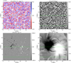 |
Fig. 1 Snapshot of the simulation after 3850 s, showing: the vertical velocity at the photosphere (panel a) the normalised intensity at 500 nm (panel b), the vertical magnetic field at the photosphere (panel c), and the vertical magnetic field at a height of 2 Mm in the chromosphere (panel d). The dashed green lines show the slices taken in Fig. 2. Panels c and d have been saturated in order to show the fine structure of the magnetic field. Slices at the photosphere are taken at the contour where τ500 = 1. |
4 Radiative Cooling and Heating
The radiative losses and heating in the simulation can be split into contributions from the multi-group scheme in and below the temperature minimum and low chromosphere, the chromospheric line losses, and the optically thin coronal losses. Figure 4 shows these different components for a slice through the model. The multi-group RT scheme cools and heats the photosphere and shocks near the temperature minimum. In the low chromosphere, the calcium and magnesium losses are strongest. The hydrogen losses are strong throughout the chromosphere, dominating the upper chromosphere and peaking in the lower transition region. The optically thin losses dominate above the transition region and are strongest in a narrow region immediately above the transition region.
The prescription for Lyman-alpha and the Lyman-continuum do not provide any heating in the upper chromosphere. The prescriptions for calcium and magnesium can provide a small amount of heating when the temperature decreases below 3.5 kK. The extreme ultraviolet (EUV) back-heating is strongest in the upper chromosphere, below the transition region, where neutral helium can form. The angle averaged intensity and heating rate of the EUV bin are shown in Fig. 5 for a slice through the simulation. High heating rates, above 1010 ergg−1 S−1, are strongly localised near areas of the transition region where the optically thin losses are high.
To investigate the relative importance of the different lines we plot the cooling/heating timescales in Fig. 6. The ionisation and recombination times in the chromosphere are long, preventing fast recombination of hydrogen as the gas is cooled. We therefore calculate the timescales τ = Einst/Q using the terms in the internal energy that can instantaneously change Einst = 3/2NkBT+EnonH+Emol,CE. This includes the microscopic kinetic energy, the ionisation of non-hydrogen species and the formation of H− and  molecules in chemical equilibrium. Figure 6 shows histograms of the timescale with temperature, for the chromospheric line losses and back-heating. Calcium cooling extends to lower temperatures, affecting shocks down to the temperature minimum, but it is lower than magnesium and hydrogen through the mid-to-high chromosphere. Magnesium cooling is strongest in regions below ≈10 kK, and hydrogen dominates radiative losses from ≈10 kK to the transition region, reaching timescales lower than 10 s. These results are similar to those presented in Carlsson & Leenaarts (2012), with hydrogen dominating the cooling above the mid chromosphere (≈ 1.5 Mm) and being marginally lower than magnesium in the low chromosphere.
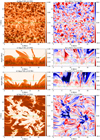 |
Fig. 2 Slices through the chromosphere after 3850 s of the simulation, showing temperature in the left column and vertical velocity in the right column. Slices in the horizontal plane are taken through the low chromosphere (panels a and b) and the upper chromosphere (panels ɡ and h). The middle rows show vertical slices through a quieter inter-network region (panels c and d) and through the centre of the network field (panels e and f). An animation is available online. |
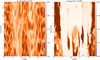 |
Fig. 3 Time-distance diagram of temperature spanning 14 min of the simulation. The slice is taken at y = 12 Mm and at two heights, z = 1 Mm (panel a) and z = 2 Mm (panel b). |
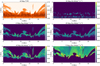 |
Fig. 4 Radiative cooling in the photosphere and chromosphere for a slice through the simulation. Panel a shows the temperature, and panel b shows the losses through the three-dimensional multi-group radiation transport scheme. The chromospheric line losses are shown for magnesium, calcium, and hydrogen in panels c, d, and e, respectively. Panel f shows the optically thin losses in the corona. |
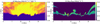 |
Fig. 5 Radiative back-heating of the upper chromosphere due to optically thin coronal losses. Panel a shows the intensity due to the coronal losses, and panel b shows the heating in the chromosphere. |
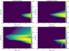 |
Fig. 6 Histograms of radiative timescales in the chromosphere with temperature, showing the recipes for calcium (panel a), magnesium (panel b), and hydrogen losses (panel c). Panel d shows the back-heating from optically thin losses in the corona. |
5 Hydrogen Populations
To investigate the effects of the NE treatment of hydrogen on the thermodynamics of the simulation we plot histograms of the temperature and electron number density in Fig. 7. The results of the NE EoS are compared to those calculated in LTE. The preferred temperature of hydrogen ionisation, around 8 kK is a prominent feature in the LTE results, but it is inconspicuous in the NLTE case. Two preferred temperature bands remain at 10 kK and 30 kK, caused by the first and second ionisation stages of helium, which is treated in LTE (Leenaarts et al. 2011; Golding et al. 2016). The spread of temperatures in the chromosphere is wider due to the long recombination timescales preventing hydrogen ionisation from buffering the temperature fluctuations. The effect of the higher ionisation fraction is also seen in the electron number density, which is higher than LTE in the low to mid chromosphere.
A detailed look at the hydrogen populations can be seen in Fig. 8. In order to compare the NE simulation with LTE we calculate the departure coefficient b of a quantity X as the ratio of the value in NE, to the value calculated using the LTE EoS, bX = XNE/XLTE. The departure coefficient of temperature (bT, panel b) shows up to 35% higher temperature in shocks and the transition region in the NE simulation, while behind the shocks the temperature is reduced by up to 25%. The ionisation fraction (panel c) is smooth throughout the chromosphere, as the long recombination timescales prevent neutral formation in the inter-shock regions. The departure coefficient for molecular hydrogen ( , panel h) is 1 in the photosphere and the temperature minimum, and around unity in cold chromospheric pockets. In warmer regions of the mid chromosphere the departure coefficient can be temporarily enhanced, and in hot shocks and the upper chromosphere it is reduced. The increase (or decrease) in H2 departure coefficient occurs largely in locations where the temperature departure coefficient is decreased (or increased). The departure coefficients of the hydrogen ground state (b1, panel e), and first excited state (b2, panel f) in the corona are b1 = 1.7 × 10⁴ and b2 = 4 × 10⁴, similar to the values of Leenaarts et al. (2007). Although small regions with b1 > 109 are seen, we do not see large regions with extremely high departure coefficients just above the transition region (b1 > 1010), as observed in Leenaarts et al. (2007). The departure coefficients of the Bifrost public simulation (Carls son et al. 2016) show similar magnitudes and behaviour as those shown in Fig. 8. They are shown for the initial snapshot, calculated from the Bifrost code, in Fig. F.1.
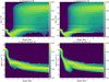 |
Fig. 7 Histograms of the temperature (top) and electron number (bottom) throughout the photosphere and chromosphere of the simulation. We compare the NE values (left columns) with those obtained from the pre-tabulated LTE EoS (right columns). |
6 Numerical Performance
In this section we investigate the numerical cost of the newly implemented routines. These simulations were performed on the Max-Planck Computation data facilities ‘Raven’ cluster. This cluster contains 1592 compute nodes, each consisting of Intel Xeon IceLake-SP processors (Platinum 8360Y) processors, with 72 cores run at 2.4 GHz and connected with Mellanox HDR InfiniBand network (100 Gbit s−1) interconnects. For the results presented in this section we used 20 nodes, or 1440 cores. The MURaM code is written with message passing interface (MPI) communication and does not support hybrid shared memory calculations.
The simulation presented in this work, row 1 of Table 1, was performed with an Alfvén speed limit of 2000 km s−1, has a typical time step of 8.89 ms. We calculated the average time per iteration from 200 time-step updates, the expected computational time per grid cell update and the cost of simulating 1 h of solar evolution. A summary of the timing, the time step and the wall time are presented in Table 1. The simulation setup shown in the paper will take 57.30 µs per grid point per core. This gives a wall time cost of approximately 1.38 million CPU-hours (Mcore-h) per hour of simulated time.
To determine the computational costs of the new physics implemented in this work we performed a number of test simulations. The simplest of these is a simulation with a LTE EoS, grey LTE multi-group RT, and no back-heating due to coronal EUV radiation. This setup, row 2 of Table 1, is similar to that presented by Rempel (2017) utilising the coronal extension to the MURaM code and costs 0.16 Mcore-h per hour of solar time (6.61 µs per grid point per core). This grey LTE simulation spends 14% of the computational time on the RT modules, 66% on MHD, and 5% and 7.5% on the EoS and diffusion treatments, respectively. By comparison, in the chromospheric simulations presented in this work, the computational cost is dominated by the EoS, and to a lesser extent the RT.
First, we consider the effects of including the extended RT modules. Including the EUV back heating of the chromosphere, row 3 of Table 1, increases the cost of RT by almost 300%. This corresponds to a 26% increase in the total computational time. This large increase is due to the optically thin nature of the EUV radiation in the corona, rays can cross many computational sub-domains and take more iterations to converge. Including a four-band scattering formulation, row 4 of Table 1, for the three-dimensional multi-group radiation scheme further increases the computational cost of the simulation by 90%. Including the more realistic treatment of RT makes RT the most expensive component of the simulation, requiring 64% of the computational time. This large increase is from additional iterations of the strongly scattering sub-bins. Most of the radiation groups converge quickly, in two or three iterations, similar to the grey radiation bin. However, the optically thin chromospheric lines bin can take up to seven iterations to converge.
The greatest computational cost is the inclusion of the NE ionisation of hydrogen in the EoS. The new module increases the total runtime by 360%. This includes the solution of the hydrogen rate equations, as well as overhead in the MHD and diffusion modules. The increase in the MHD and diffusion modules is caused by advection and diffusion of the atomic populations, and calls to the EoS to maintain consistency of the solution between directional sweeps of the diffusion routine. The simulation setup presented in this paper requires 8.6 times more computational power per grid point than the LTE coronal simulations presented in Rempel (2017).
In addition, we varied two approximations that have a significant effect on the computational cost. Firstly, we performed two simulations where the minimum limit on the speed of light is changed. Increasing the speed of light, to 5000 km s−1, row 5 of Table 1, reduces the time step leading to a 230% increase in the computational cost. Reducing the speed of light to 1000 km s−1, row 6 of Table 1, allows a larger time step and lowers the computational cost by 37%.
A second choice that affects the computational cost is the frequency (in iterations) at which the radiation field is calculated. Updating the radiation field every iteration, row 7 of Table 1, increases the computational cost of RT by 300%. Reducing the frequency to every 10 iterations, row 8 of Table 1, reduces it by 40%. This change does not scale linearly as more iterations are needed to converge the radiation field to the required tolerance when it is calculated less regularly.
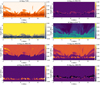 |
Fig. 8 Properties of the NE hydrogen populations through the centre of the enhanced network region. The panels show (a) temperature in the NE simulations, (b) the departure coefficient of temperature, bT = Tne/Tlte, (c) the NE ionisation fraction, Fi = nH,1/nH,tot, (d) the number density of the first excited level of hydrogen, nH,0,1, and departure coefficients of (e) the ground state, (f) the first excited state, (g) protons, and (h) molecular hydrogen. |
Simulation setups.
7 Discussion and Conclusion
The current work improves on the original LTE MURaM code through the implementation of three new modules: an NE treatment of hydrogen in the EoS, NLTE tabulated losses in the chromosphere, and a scattering multi-group RT scheme. An initial simulation has been performed, beginning from the publicly available Bifrost snapshot. The simulation differs significantly from the original Bifrost model due to differences in the diffusion scheme, the potential boundary condition, and small differences in the EoS. A detailed comparison between the results from Bifrost and MURaM will be the subject of a separate paper.
The simulation shows the importance of an NE treatment of hydrogen in the chromosphere. The upper chromosphere is highly dynamic, with strong shocks and large departure coefficients of the ground state and n = 2 energy level. Despite the strong gradients and fine structure in velocity and temperature, the hydrogen populations in the upper atmosphere are smooth due to the long recombination times, relative to the dynamical timescales. The departure coefficients b1 and b2 are approximately 103 to 106 in the upper chromosphere. The calculated departure populations match those in the Bifrost code (Leenaarts et al. 2007; Carlsson et al. 2016). The temperatures are around 25% different from the LTE values, and the electron number density remains higher in cold shock expansions. These differences occur due to the inability of protons to recombine into neutral hydrogen before a new shock passes through the chromosphere. These differences will be important for the accurate synthesis of chromospheric spectral lines.
The current implementation of chromospheric radiative losses and the NE EoS are based upon a number of simplifying assumptions:
The tabulated chromospheric line losses ignore significant scatter around pre-tabulated values of escape probability, the ionisation fraction, and the radiative loss function. The optically thin formalism cannot simulate three-dimensional heating effects due to shocks and explosive events;
The radiation field used for the NE treatment of hydrogen is isotropic in the chromosphere;
The treatment of Lyman-alpha in radiative equilibrium for the NE treatment of hydrogen is inaccurate near the transition region (Carlsson & Stein 2002; Golding et al. 2016);
Atomic and molecular populations in the multi-group radiation transport scheme are treated in LTE;
Helium is treated in LTE.
The above approximations are necessary for the simulation of large three-dimensional models that include an NE chromosphere. They will also have a significant effect on the physics and chemistry acting in the chromosphere. It is important to investigate new methods to relax these assumptions. The work by Golding et al. (2016) has extended the NE EoS and chromospheric line cooling to be more accurate in the upper chromosphere and transition region. This includes an approximate Lyman-alpha bin, allowing for three-dimensional cooling and heating effects while ignoring scattering and PRD effects. Additionally, the optically thin losses have been split into six EUV frequency bands to incorporate the Lyman continuum and a simplified three-level helium atom. These improvements greatly increase the realism of the method in the upper chromospheric layers.
Another proposal for the fast NE treatment of atoms in a radiative MHD simulation is described by Judge (2017). This method uses the escape probability approach to quickly converge the populations. The method is easily extendable to elements other than hydrogen. The one-dimensional plane-parallel nature may lead to unrealistic variations between neighbouring horizontal pixels. It is also suggested that the EoS be decoupled from atomic populations and the problem solved in stages, where the populations are updated and then used to calculate the new temperature, electron number density, and pressure. This would reduce the complexity of the system of equations that are solved and allow the use of a pre-tabulated EoS, potentially offering a significant increase in speed when solving the NE problem.
Finally, a new time-implicit numerical method for solving the detailed NE radiative MHD problem, built as an extension to the MURaM code, is presented in Anusha et al. (2021). The formulation allows larger time steps to be taken when solving the system of rates, making the method promising for time-dependent multi-dimensional simulations.
Recent studies (Martinez-Sykora et al. 2012; Shelyag et al. 2016) have shown the importance of including ion-neutral interactions, in particular ambipolar diffusion, in simulations of the chromosphere. The collisional rates and electron number density are strongly tied to the hydrogen ionisation fraction, and this varies greatly between LTE and NE. Including NE ionisation reduces the impact of ambipolar diffusion on the simulation; however, a decreased efficiency of shock heating is observed, as is the heating of cool low-lying loops (Martinez-Sykora et al. 2020). Ambipolar diffusion and the Hall effect are included in the MURaM code (Cheung & Cameron 2012; Rempel & Przybylski 2021), and simulations that include both effects will soon be performed.
Movie
Movie 1 associated with Fig. 2 (fig2_movie) Access Supplementary Material
Acknowledgements
We thank the anonymous referee for suggestions that improved the paper. We would like to thank S. Danilovic for assisting with understanding of the MURaM code and facilitating collaboration with the Stockholm group. D.P. would like to acknowledge the help of I. Milic, K. Sowmya, H.N. Smitha, M. van Noort, R. Collet, and P. Judge for helpful discussion relating to NLTE and NE physics. D.P. would also like to thank the Bifrost group for helpful explanations of the Bifrost code, especially V. Hansteen. This project has received funding from the European Research Council (ERC) under the European Union’s Horizon 2020 research and innovation programme (grant agreement No. 695075). We gratefully acknowledge the computational resources provided by the Cobra & Raven supercomputer systems of the Max Planck Computing and Data Facility (MPCDF) in Garching, Germany. J.L. was supported by a grant from the Knut and Alice Wallenberg foundation (2016.0019). This material is based upon work supported by the National Center for Atmospheric Research, which is a major facility sponsored by the National Science Foundation under Cooperative Agreement No. 1852977. L.S.A., V.W., and A.I.S. acknowledge support from the European Research Council (ERC) under the European Union’s Horizon 2020 research and innovation program (grant no. 715947).
Appendix A LTE Equation of State
The ideal EoS is pre-tabulated to calculate the thermodynamic variables ne, T, and p in terms of density ρ and internal energy ϵ. To start, we calculate the LTE ionisation fractions for a given density ρ, electron number ne, temperature T and set of abundances Aa, using the Saha-Boltzmann equation:
 (A.1)
(A.1)
where kB is Boltzmann’s constant, me the electron mass, h is Planck’s constant and Δμ the ionisation lowering due to interactions with surrounding particles. Ua,i is the partition function, χa,i the ionisation energy, Za,i the charge, and and na,i the number density for element a and ionisation stage i. Where available, we used the polynomial partition functions of Cardona et al. (2005), except for iron and nickel where the tables of Halenka et al. (2001) and Halenka & Madej (2002) were used. The H− fraction was calculated from Eq. (A.1) and the H2 and  fractions are
 (A.2)
(A.2)
 (A.3)
(A.3)
where m is the reduced mass and  and
and  are the dissociation energies. The partition functions of H2 were taken from (Popovas & Jørgensen 2016) and the partition functions of
  are from a polynomial fit to the Stancil ((1994) table. Following Mihalas et al. (1988), the energy of the hydrogen species are
 (A.4)
(A.4)
 (A.5)
(A.5)
 (A.6)
(A.6)
 (A.7)
(A.7)
where χH,i,e is the excitation or ionisation energy of the hydrogen level (i, e). The ionisation energy of neutral hydrogen is χH,1 = 13.59844 ev, and for H− is χH,−1 = 0.754 ev. Once the fractions of all elements and of the hydrogen molecules are determined we followed the formulation of the VMW EoS. This process involves iterating the ionisation and molecular fractions, electron number density and temperature until a convergence criteria is reached. We iterated this procedure until the electron number density converged to a tolerance of 1.0 × 10⁻⁸. Once converged, the energy and pressure are calculated
 (A.8)
(A.8)
 (A.9)
(A.9)
in terms of excitation and ionisation (exi), translational (trans), radiation (rad), Coloumb (C), and pressure ionisation (PI) components. We ignore the effects of degenerate and relativistic electrons as they are small within the physical regime of these simulations. The radiation energy and pressure terms are also small and not included. The translational components are calculated as ptrans = (Σa,i na,i + ne) kBT and Etrans = 3/2 ptrans.
The contribution to the energy from excitation and ionisation is calculated as
 (A.10)
For the Coulomb correction we followed the prescription of Mihalas et al. (1988). The free energy, ignoring electron density, is calculated for a parcel of gas of volume V and a particle number N = nV as
 (A.11)
where the function τ is
 (A.12)
and x is given by
 (A.13)
The required derivatives of τ and x are
 (A.14)
 (A.15)
 (A.16)
 (A.17)
The reduction of the ionisation potential ΔµC, used in the Saha-Boltzmann equation (Eq. (A.1)), is
 (A.18)
giving a pressure correction of
 (A.19)
and an internal energy correction of
 (A.20)
Simplifying Eqs. A.19–A.20 and taking V = 1.0 cm−3 gives
 (A.21)
 (A.22)
 (A.23)
Additionally, the pressure ionisation device described in the Eggleton, Faulkner, and Flannery EoS (Eggleton et al. 1973) was included. This method provides a thermodynamically consistent result that gives a qualitatively correct pressure ionisation as density increases:
 (A.24)
where Ne,0 is the electron number of the gas when it is fully ionised and Ω is
 (A.25)
where a0 = 5.23e−9/〈Z〉 cm, χ0 = 2.16e−11 〈Z〉2 erg, and 〈Z〉 is the mean charge per nucleus and the required derivative,
 (A.26)
The change in the potential can then be calculated as
 (A.27)
the pressure correction as
 (A.28)
and finally the internal energy correction as
 (A.29)
Once a complete solution is obtained for all required density and energy values, the entropy s is calculated by integrating over the table,
 (A.30)
Appendix B Derivatives of the Non-Equilibrium Equation of State
EoS derivatives for chemical equilibrium of  ,
,
 (B.1)
(B.1)
 (B.2)
(B.2)
 (B.3)
(B.3)
and for H−1,
 (B.4)
(B.4)
 (B.5)
(B.5)
 (B.6)
(B.6)
The derivatives for the energy conservation equation, ƒ0, are
![Mathematical equation: $ \matrix{ {{{\partial {f_0}} \over {\partial T}}} \hfill & { = - {1 \over {{E_{{\mathop{\rm int}} }}}}\left( {{{3{k_{\rm{B}}}} \over 2}\left[ {{n_{\rm{e}}} + {n_{{\rm{nonH}}}} + {n_{{{\rm{H}}_{\rm{2}}}}} + {n_{{{\rm{H}}_{{\rm{2,1}}}}}}} \right.} \right.} \hfill \cr {} \hfill & { + {n_{{\rm{H, - 1}}}} + \sum\limits_{i,j} {{n_{{\rm{H}},i,j}}} \left] { + {{3{k_{\rm{B}}}T} \over 2}} \right[{{\partial {n_{noH}}} \over {\partial T}} + {{\partial {n_{{\rm{H, - 1}}}}} \over {\partial T}}} \hfill \cr {} \hfill & {\left. { + {{\partial {n_{{{\rm{H}}_2},1}}} \over {\partial T}}} \right] + {n_{{\rm{H,tot}}}}{{\partial {E_{{\rm{nonH}}}}} \over {\partial T}} + {{\partial {E_{{{\rm{H}}_2}}}} \over {\partial T}}{n_{{{\rm{H}}_2}}}} \hfill \cr {} \hfill & {\left. { + {{\partial {E_{{\rm{H, - 1}}}}{n_{{\rm{H, - 1}}}}} \over {\partial T}} + {{\partial {E_{{H_{2,1}}}}{n_{{{\rm{H}}_{2,1}}}}} \over {\partial T}}} \right),} \hfill \cr } $](/articles/aa/full_html/2022/08/aa41230-21/aa41230-21-eq94.png) (B.7)
(B.7)
![Mathematical equation: $ \matrix{ {{{\partial {f_0}} \over {\partial {n_{\rm{e}}}}}} \hfill & { = - {1 \over {{E_{{\mathop{\rm int}} }}}}\left( {{{3{k_{\rm{B}}}T} \over 2}\left[ {1.0 + {{\partial {n_{{\rm{H,}} - 1}}} \over {\partial {n_{\rm{e}}}}}} \right] + {n_{{\rm{H,tot}}}}{{\partial {E_{{\rm{nonH}}}}} \over {\partial {n_{\rm{e}}}}}} \right.} \hfill \cr {} \hfill & {\left. { + {{\partial {n_{{\rm{H,}} - 1}}} \over {\partial {n_{\rm{e}}}}}{E_{{\rm{H, - 1}}}}} \right),} \hfill \cr } $](/articles/aa/full_html/2022/08/aa41230-21/aa41230-21-eq95.png) (B.8)
(B.8)
 (B.9)
(B.9)
 (B.10)
The derivatives for the charge conservation equation, f1 , are
 (B.11)
 (B.12)
 (B.13)
 (B.14)
The derivatives for the hydrogen nucleus conservation equation, f2 , are
 (B.15)
 (B.16)
 (B.17)
 (B.18)
The derivatives of the rate-equations, f2+i, are
 (B.19)
 (B.20)
 (B.21)
 (B.22)
 (B.23)
Appendix C Rate Equations for Solution of Non-Equilibrium Hydrogen
The radiative rates used in this work were calculated using the prescription of Sollum (1999) (see also Leenaarts & Wedemeyer-Böhm 2006 for a description of their implementation in a three-dimensional simulation). The angle averaged radiation field Jv for each transition is given in terms of a height-dependent radiation temperature Trad by setting Jν = Bv (Trad), where
 (C.1)
(C.1)
In the upper atmosphere Trad is constant, using the values (TSol) prescribed for each transition. These values were chosen to match comprehensive one-dimensional RADYN simulations (Sollum 1999). Below the photosphere Trad is equal to the local gas temperature T, these are smoothly joined by setting
![Mathematical equation: $ {J_{{T_{{\rm{rad}}}}}}\left( z \right) = {B_v}\left( {{T_{{\rm{sol}}}}} \right) + \left[ {{B_v}\left( {{T_{{\rm{crit}}}}} \right) - {B_v}\left( {{T_{{\rm{sol}}}}} \right)} \right]{\left( {{{{m_c}\left( z \right)} \over {{m_{{\rm{c,crit}}}}}}} \right)^{{H_{{\rm{sol}}}}}} $](/articles/aa/full_html/2022/08/aa41230-21/aa41230-21-eq112.png) (C.2)
(C.2)
in terms of column mass mc, and as well as a cutoff temperature Tcrit and column mass mc,crit. The parameter HSol was defined for each transition, and fit to a Radyn simulation by Sollum (1999). The critical values of temperature and column mass were determined by finding the lowest point (zcrit) for which Bv (T) = 2Bv (TSol). Below this point Trad = T and above it we used Eqs. C.1 and C.2 to calculate Trad. This method decouples the radiation field from the thermodynamic properties, allowing a rapid calculation and fast convergence of the hydrogen populations.
The radiative rates can then be calculated from Trad and Jv (see Sollum 1999 for a detailed derivation). For a lower level, l, and an upper level, u, the upwards, Rl,u, and downwards, Ru,l, radiative rates are
 (C.3)
(C.3)
 (C.4)
(C.4)
where e is the electron charge, gi the statistical weight of level i, fl,u is the oscillator strength, and v0 is the line centre frequency. The radiation temperature Trad = T when z < zcrit and is constant when z > zcrit. The temperature derivative of Jv is
 (C.5)
(C.5)
and the derivatives of the bound-bound rates are
 (C.6)
(C.6)
 (C.7)
(C.7)
The bound-free rates between a lower level, l, and continuum 6 are
 (C.8)
(C.8)
![Mathematical equation: $ \matrix{ {{R_{6,l}}} \hfill & = \hfill & {{R_{l,6}}{{\left[ {{{{n_l}} \over {{n_6}}}} \right]}_{LT\,E}},for\,z < {z_{{\rm{crit}}}}} \hfill \cr {} \hfill & = \hfill & {{{8\pi } \over {{c^2}}}{\alpha _0}v_0^3{{\left[ {{{{n_l}} \over {{n_6}}}} \right]}_{LT\,E}}} \hfill \cr {} \hfill & {} \hfill & {\sum\limits_{n = 0}^\infty {{E_1}\left( {\left[ {n{T \over {{T_{{\rm{rad}}}}}} + 1} \right]{{h{v_0}} \over {{k_{\rm{B}}}T}}} \right),{\rm{for}}\,z \ge {z_{{\rm{crit}}}},} } \hfill \cr } $](/articles/aa/full_html/2022/08/aa41230-21/aa41230-21-eq119.png) (C.9)
(C.9)
where ![Mathematical equation: ${\left[ {{{{n_l}} \over {{n_6}}}} \right]_{LT\,E}}$](/articles/aa/full_html/2022/08/aa41230-21/aa41230-21-eq120.png) is the LTE population ratio and α0 is the radiative absorption cross-section at the ionisation edge frequency, ν0. The derivatives of the bound-free rates are
is the LTE population ratio and α0 is the radiative absorption cross-section at the ionisation edge frequency, ν0. The derivatives of the bound-free rates are
 (C.10)
![Mathematical equation: $ \matrix{ {{{\partial {R_{l,6}}} \over {\partial T}}} \hfill & { = {{\partial {R_{l,6}}} \over {\partial T}}{{\left[ {{{{n_l}} \over {{n_6}}}} \right]}_{LT\,E}}} \hfill \cr {} \hfill & { - {R_{6,l}}\left( {{3 \over {2T}} + {{h{v_0}} \over {{k_{\rm{B}}}{T^2}}}} \right),\,{\rm{for}}\,z\, \ge {z_{{\rm{crit}}}}} \hfill \cr {} \hfill & { = {{8\pi } \over {{c^2}}}{\alpha _0}v_0^3{{\left[ {{{{n_l}} \over {{n_6}}}} \right]}_{LT\,E}}\sum\limits_{n = 0}^\infty {{{\exp \left( { - {{nh{v_0}} \over {{k_{\rm{B}}}{T_{{\rm{rad}}}}}} - {{h{v_0}} \over {{k_{\rm{B}}}T}}} \right)} \over {nT + {T_{{\rm{rad}}}}}}} {T \over {{T_{{\rm{rad}}}}}}} \hfill \cr {} \hfill & { - {R_{6,l}}\left( {{3 \over {2T}} + {{h{v_0}} \over {{k_{\rm{B}}}{T^2}}}} \right),{\rm{for }}z \ge {z_{crit}},} \hfill \cr } $](/articles/aa/full_html/2022/08/aa41230-21/aa41230-21-eq122.png) (C.11)
(C.11)
 (C.12)
 (C.13)
In Fig. C.1 we compare detailed SE calculations made with the Rybicki-Hummer (RH) code (Uitenbroek 2001; Pereira & Uitenbroek 2015) to those using the Sollum radiative rates. We use the Fontenla-Avrett-Loeser Quiet Sun model-C (FAL-C) atmosphere (Fontenla et al. 1993). The SE solution calculated using the Sollum rates closely match the detailed solution for much of the photosphere up to the mid chromosphere. In the upper chromosphere, the Sollum treatment of Lyman lines in detailed balance leads to a higher ionisation fraction and a lower population in the first excited state. When Lyman lines are treated in detailed balance in the RH calculation, the result closely matches that from the Sollum rates.
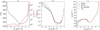 |
Fig. C.1 Statistical equilibrium populations of hydrogen, comparing the Sollum radiative rates with a detailed calculation using the RH code. Panel (a) shows the temperature and electron density of the FAL-C atmosphere. Panel (b) compares the ionisation fraction and panel (c) the n2 populations. These are shown for LTE (dashed red lines) and the Sollum radiative rates (dashed blue lines) as well as from two detailed calculations with the RH code, one that treats Lyman lines in detailed balance (dashed green lines) and a second that calculates the radiative rates for the Lyman lines (solid black lines; see the legend in panel c). |
Appendix D Molecular Hydrogen Rates
For the time-dependent solution of the molecular H2 we used a set of rates described in Table D, these are often described in terms of the Arrhenius equation,
 (D.1)
(D.1)
and its derivative,
 (D.2)
(D.2)
The rate coefficients, K, are used in the equations of molecular hydrogen and the hydrogen ground state. In the case of K6 and K7, the H− and  molecules were assumed to automatically dissociate.
Molecular hydrogen formation and dissociation rates.
Appendix E Opacity Binning
To create the group-integrated opacities for the multi-group scattering scheme we require the absorption (κ), scattering (σ) and total (χ = σ + κ) opacities. The opacity contains a contribution from the continuum c and from lines l. Detailed opacity distribution functions (ODFs) were taken from the merged parallelised simplified ATLAS code (Witzke et al. 2021), an upgraded version of ATLAS9 (Kurucz 1970). For the continuum, the total and scattering opacities are available through the ATLAS package, tabulated with frequency, temperature and pressure. For the spectral line contribution, ODFs are used. The ODFs are tabulated on the same frequency, temperature and pressure grid as the continuum values, with an additional 12 sub-bins per frequency point. To extract the absorption and scattering opacity from the total opacity in the ODFs we followed Skartlien (2000), using the approximation of van Regemorter (1962). The photon destruction probability of a frequency, ν, is given by the probability for collisional de-excitation from the upper level, j, to the lower level, i:
 (E.1)
(E.1)
Here Aj,i is the Einstein coefficient for spontaneous radiative de-excitation and Cj,i is the collisional de-excitation parameter. Using van Regemorter’s approximation,
 (E.2)
(E.2)
where the function  is pre-tabulated by van Regemorter (1962). This allows the scattering and absorption opacities to be determined using
  :
:
 (E.3)
(E.3)
 (E.4)
(E.4)
The total opacities are then calculated:
 (E.5)
(E.5)
 (E.6)
(E.6)
For each band j of the multi-group scheme, consisting of a set of frequencies Ωj = {ν}, different averages are used to calculate the group-integrated opacities (see Skartlien 2000 for a detailed discussion). These are the Rosseland mean opacity,  ,
,
 (E.7)
(E.7)
the Planck mean opacity, 
 (E.8)
(E.8)
and the intensity-weighted meam,  ,
,
 (E.9)
(E.9)
in terms of a mean intensity Jpp, calculated for each bin of the ODF This was performed using a one-dimensional plane-parallel reference atmosphere and a short-characteristics scheme, similar to that used in the MURaM code, with  and arbitrary azimuths. In this work we used an atmosphere calculated using a column mass average of the full time-series of the Bifrost public release (Carlsson et al. 2016), shown in Fig. E.1. To extrapolate from the one-dimensional Jpp to the full range of p, Τ a reference optical depth was used, we used τ500.
The extrapolation was performed following a procedure similar to that described by (Collet et al. 2011). For each x, y pixel of each snapshot of the reference simulation time series we binned τ500 values for temperature and pressure corresponding to the ODF grid. Additionally, we calculate a column mass averaged atmosphere of the three-dimensional simulation. The log-mean  was calculated for each temperature and pressure point in the table. This
  was interpolated to fill any gaps and then extrapolated to the full range of temperature and pressure used in the ODF table. The column-mass averaged background model was used to calculate
  and Jpp. Using the assumption that Jpp is constant over points with the same optical depth (τ500) the intensity mean was calculated for the full table.
The resulting background model, extrapolated  , intensity Jpp and photon destruction probability ϵ can be seen in Fig. E.1.
We then followed the formalism of Ludwig (1992) to join the diffusion (optically thick) and streaming (optically thin) domains. Firstly the extinction coefficient is given as
 (E.10)
where τ0 =0.1 and the group optical depth τj is approximated using the expression
 (E.11)
where g⊙ is the gravity at the photosphere. Similarly, the scattering albedo is
 (E.12)
and the integrated emissivity is
 (E.13)
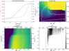 |
Fig. E.1 Atmospheric properties required to calculate the multi-group scattering opacities. Panel (a): Density and temperature of the reference atmosphere. Panel (b): Binned optical depth, |

Appendix F Initial Hydrogen Populations
In Fig. 8 we show the departure coefficients from the initial snapshot, which was computed in Bifrost code (Carlsson et al. 2016). This snapshot is used as the initial condition for the simulation presented in this paper. The departure coefficients are seen in Fig. F.1. The H2 populations are very small in the upper chromosphere, and the large departure coefficients are energetically and dynamically insignificant.
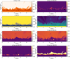 |
Fig. F.1 Properties of the NE hydrogen populations in the initial snapshot, through the centre of the enhanced network region. The panels show (a) temperature in the NE simulations, (b) the departure coefficient of temperature, bT = TNE/TLTE, (c) the NE ionisation fraction, Fi = nH,1/nH,tot, (d) the number density of the first excited level of hydrogen, nH,0,1, and the departure coefficients of (e) the ground state, (f) the first excited state, (g) protons, and (h) molecular hydrogen. |
Appendix G Comparison to RH
In order to test if the code correctly reproduces the limiting LTE and coronal equilibrium cases we performed the test from Sect. 11.6 of Gudiksen et al. (2011). In Fig. G.1 we compare the hydrogen populations of the MURaM NE module with those calculated in SE in RH (Uitenbroek 2001; Pereira & Uitenbroek 2015). The ground state population dendsities match the SE calculation for the interior and low chromosphere. In the upper-chromosphere the ground state population varies strongly from the SE solution, and in the corona the proton number differs, although variations remain within a factor of 10. The proton densities match the SE calculation for the interior, transition region and corona. Throughout the chromosphere the proton number densities differ strongly from the SE solution.
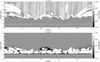 |
Fig. G.1 Comparison of the ground state (panel a) and proton (panel b) number densities from the MURaM NE treatment of hydrogen and 1.5D SE calculations using the RH code. |
References
- Anusha, L.S., van Noort, M., & Cameron, R.H. 2021, ApJ, 911, 71 [NASA ADS] [CrossRef] [Google Scholar]
- Beeck, B., Collet, R., Steffen, M., et al. 2012, A&A, 539, A121 [NASA ADS] [CrossRef] [EDP Sciences] [Google Scholar]
- Beeck, B., Cameron, R.H., Reiners, A., & Schüssler, M. 2013, A&A, 558, A48 [NASA ADS] [CrossRef] [EDP Sciences] [Google Scholar]
- Beeck, B., Schüssler, M., Cameron, R.H., & Reiners, A. 2015, A&A, 581, A42 [NASA ADS] [CrossRef] [EDP Sciences] [Google Scholar]
- Boris, J.P. 1970, NRL Memorandum Report 2167 (Naval Research Lab: Washington DC) [Google Scholar]
- Bruls, J.H.M.J., Vollmöller, P., & Schüssler, M. 1999, A&A, 348, 233 [NASA ADS] [Google Scholar]
- Cannon, C.J. 1973, ApJ, 185, 621 [NASA ADS] [CrossRef] [Google Scholar]
- Cardona, O., Simonneau, E., & Crivellari, L. 2005, Rev. Mex. Fisica, 51, 476 [Google Scholar]
- Carlson, B.G. 1963, in Methods in Computational Physics, eds. B. Alder, & S. Fernbach, 1 [Google Scholar]
- Carlsson, M., & Leenaarts, J. 2012, A&A, 539, A39 [NASA ADS] [CrossRef] [EDP Sciences] [Google Scholar]
- Carlsson, M., & Stein, R.F. 1992, ApJ, 397, L59 [Google Scholar]
- Carlsson, M., & Stein, R.F. 2002, ApJ, 572, 626 [NASA ADS] [CrossRef] [Google Scholar]
- Carlsson, M., Hansteen, V.H., Gudiksen, B.V., Leenaarts, J., & De Pontieu, B. 2016, A&A, 585, A4 [NASA ADS] [CrossRef] [EDP Sciences] [Google Scholar]
- Chen, F., Rempel, M., & Fan, Y. 2017, ApJ, 846, 149 [Google Scholar]
- Cheung, M.C.M., & Cameron, R.H. 2012, ApJ, 750, 6 [NASA ADS] [CrossRef] [Google Scholar]
- Cheung, M.C.M., Schüssler, M., & Moreno-Insertis, F. 2007, A&A, 467, 703 [CrossRef] [EDP Sciences] [Google Scholar]
- Cheung, M.C.M., Rempel, M., Chintzoglou, G., et al. 2019, Nat. Astron., 3, 160 [NASA ADS] [CrossRef] [Google Scholar]
- Collet, R., Hayek, W., Asplund, M., et al. 2011, A&A, 528, A32 [NASA ADS] [CrossRef] [EDP Sciences] [Google Scholar]
- Danilovic, S. 2017, A&A, 601, A122 [NASA ADS] [CrossRef] [EDP Sciences] [Google Scholar]
- Dedner, A., Kemm, F., Kröner, D., et al. 2002, J. Comput. Phys., 175, 645 [Google Scholar]
- de la Cruz Rodriguez, J., & Piskunov, N. 2013, ApJ, 764, 33 [NASA ADS] [CrossRef] [Google Scholar]
- Eggleton, P.P., Faulkner, J., & Flannery, B.P. 1973, A&A, 23, 325 [Google Scholar]
- Fontenla, J.M., Avrett, E.H., & Loeser, R. 1993, ApJ, 406, 319 [NASA ADS] [CrossRef] [Google Scholar]
- Forrey, R.C. 2013, ApJ, 773, L25 [NASA ADS] [CrossRef] [Google Scholar]
- Galli, D., & Palla, F. 1998, A&A, 335, 403 [NASA ADS] [Google Scholar]
- Golding, T.P., Leenaarts, J., & Carlsson, M. 2016, ApJ, 817, 125 [NASA ADS] [CrossRef] [Google Scholar]
- Gombosi, T.I., Töth, G., De Zeeuw, D.L., et al. 2002, J. Comput. Phys., 177, 176 [NASA ADS] [CrossRef] [Google Scholar]
- Gudiksen, B.V., Carlsson, M., Hansteen, V.H., et al. 2011, A&A, 531, A154 [NASA ADS] [CrossRef] [EDP Sciences] [Google Scholar]
- Gustafsson, B., Bell, R.A., Eriksson, K., & Nordlund, A. 1975, A&A, 42, 407 [Google Scholar]
- Halenka, J., & Madej, J. 2002, Acta Astron., 52, 195 [NASA ADS] [Google Scholar]
- Halenka, J., Madej, J., Langer, K., & Mamok, A. 2001, Acta Astron., 51, 347 [NASA ADS] [Google Scholar]
- Hayek, W., Asplund, M., Carlsson, M., et al. 2010, A&A, 517, A49 [NASA ADS] [CrossRef] [EDP Sciences] [Google Scholar]
- Hirasawa, T. 1969, Progr. Theoret. Phys., 42, 523 [CrossRef] [Google Scholar]
- Jameson, A. 2017, AIAA J., 55, 1487 [NASA ADS] [CrossRef] [Google Scholar]
- Judge, P.G. 2005, J. Quant. Spec. Radiat. Transf., 92, 479 [NASA ADS] [CrossRef] [Google Scholar]
- Judge, P.G. 2017, ApJ, 851, 5 [NASA ADS] [CrossRef] [Google Scholar]
- Kurucz, R.L. 1970, SAO Special Report, 309 [Google Scholar]
- Leenaarts, J., & Wedemeyer-Böhm, S. 2006, A&A, 460, 301 [NASA ADS] [CrossRef] [EDP Sciences] [Google Scholar]
- Leenaarts, J., Carlsson, M., Hansteen, V., & Rutten, R.J. 2007, A&A, 473, 625 [NASA ADS] [CrossRef] [EDP Sciences] [Google Scholar]
- Leenaarts, J., Carlsson, M., Hansteen, V., & Gudiksen, B.V. 2011, A&A, 530, A124 [NASA ADS] [CrossRef] [EDP Sciences] [Google Scholar]
- Ludwig, H.G. 1992, PhD thesis, Christian-Albrecht University of Kiel, Germany [Google Scholar]
- Martinez-Sykora, J., De Pontieu, B., & Hansteen, V. 2012, ApJ, 753, 161 [CrossRef] [Google Scholar]
- Martinez-Sykora, J., Leenaarts, J., De Pontieu, B., et al. 2020, ApJ, 889, 95 [NASA ADS] [CrossRef] [Google Scholar]
- McElroy, D., Walsh, C., Markwick, A.J., et al. 2013, A&A, 550, A36 [NASA ADS] [CrossRef] [EDP Sciences] [Google Scholar]
- Mihalas, D. 1967, Methods Comput. Phys., 7, 1 [NASA ADS] [Google Scholar]
- Mihalas, D., Dappen, W., & Hummer, D.G. 1988, ApJ, 331, 815 [NASA ADS] [CrossRef] [Google Scholar]
- Nordlund, A. 1982, A&A, 107, 1 [Google Scholar]
- Palla, F., Salpeter, E.E., & Stahler, S.W. 1983, ApJ, 271, 632 [NASA ADS] [CrossRef] [Google Scholar]
- Panja, M., Cameron, R., & Solanki, S.K. 2020, ApJ, 893, 113 [CrossRef] [Google Scholar]
- Pereira, T.M.D., & Uitenbroek, H. 2015, A&A, 574, A3 [NASA ADS] [CrossRef] [EDP Sciences] [Google Scholar]
- Popovas, A., & Jorgensen, U.G. 2016, A&A, 595, A130 [NASA ADS] [CrossRef] [EDP Sciences] [Google Scholar]
- Rempel, M. 2014, ApJ, 789, 132 [Google Scholar]
- Rempel, M. 2017, ApJ, 834, 10 [Google Scholar]
- Rempel, M., & Przybylski, D. 2021, ApJ, 923, 79 [NASA ADS] [CrossRef] [Google Scholar]
- Rempel, M., Schüssler, M., Cameron, R.H., & Knölker, M. 2009, Science, 325, 171 [CrossRef] [Google Scholar]
- Rogers, F.J., Swenson, F.J., & Iglesias, C.A. 1996, ApJ, 456, 902 [NASA ADS] [CrossRef] [Google Scholar]
- Schüssler, M., & Vögler, A. 2006, ApJ, 641, L73 [Google Scholar]
- Schüssler, M., Shelyag, S., Berdyugina, S., Vögler, A., & Solanki, S.K. 2003, ApJ, 597, L173 [CrossRef] [Google Scholar]
- Shapiro, A.I., Solanki, S.K., Krivova, N.A., et al. 2017, Nat. Astron., 1, 612 [NASA ADS] [CrossRef] [Google Scholar]
- Shelyag, S., Schüssler, M., Solanki, S.K., & Vögler, A. 2007, A&A, 469, 731 [NASA ADS] [CrossRef] [EDP Sciences] [Google Scholar]
- Shelyag, S., Khomenko, E., de Vicente, A., & Przybylski, D. 2016, ApJ, 819, L11 [Google Scholar]
- Skartlien, R. 2000, ApJ, 536, 465 [NASA ADS] [CrossRef] [Google Scholar]
- Sollum, E. 1999, Master's thesis, University of Oslo, Norway [Google Scholar]
- Stancil, P.C. 1994, ApJ, 430, 360 [NASA ADS] [CrossRef] [Google Scholar]
- Sukhorukov, A.V., & Leenaarts, J. 2017, A&A, 597, A46 [NASA ADS] [CrossRef] [EDP Sciences] [Google Scholar]
- Uitenbroek, H. 2001, ApJ, 557, 389 [Google Scholar]
- van Regemorter, H. 1962, ApJ, 136, 906 [NASA ADS] [CrossRef] [Google Scholar]
- Vardya, M.S. 1965, MNRAS, 129, 205 [NASA ADS] [CrossRef] [Google Scholar]
- Vitas, N., & Khomenko, E. 2015, Annales Geophysicae, 33, 703 [NASA ADS] [CrossRef] [Google Scholar]
- Vögler, A., & Schüssler, M. 2007, A&A, 465, L43 [Google Scholar]
- Vögler, A., Bruls, J.H.M.J., & Schüssler, M. 2004, A&A, 421, 741 [NASA ADS] [CrossRef] [EDP Sciences] [Google Scholar]
- Vögler, A., Shelyag, S., Schüssler, M., et al. 2005, A&A, 429, 335 [Google Scholar]
- Warnecke, J., & Bingert, S. 2020, Geophys. Astrophys. Fluid Dyn., 114, 261 [NASA ADS] [CrossRef] [Google Scholar]
- Wittmann, A. 1974, Sol. Phys., 35, 11 [Google Scholar]
- Witzke, V., Shapiro, A.I., Cernetic, M., et al. 2021, A&A, 653, A65 [NASA ADS] [CrossRef] [EDP Sciences] [Google Scholar]
- Yeo, K.L., Solanki, S.K., Norris, C.M., et al. 2017, Phys. Rev. Lett., 119, 9.1102 [Google Scholar]
- Zhang, B., Sorathia, K.A., Lyon, J.G., et al. 2019, ApJS, 244, 20 [NASA ADS] [CrossRef] [Google Scholar]
Max-Planck-Institute for Solar System Research/University of Chicago Radiation Magneto-hydrodynamics.
The tables for the chromospheric lines are available as part of an IRIS data release http://iris.lmsal.com/bf/code.tar.bz2
Animation available online
All Tables
All Figures
|
Fig. 1 Snapshot of the simulation after 3850 s, showing: the vertical velocity at the photosphere (panel a) the normalised intensity at 500 nm (panel b), the vertical magnetic field at the photosphere (panel c), and the vertical magnetic field at a height of 2 Mm in the chromosphere (panel d). The dashed green lines show the slices taken in Fig. 2. Panels c and d have been saturated in order to show the fine structure of the magnetic field. Slices at the photosphere are taken at the contour where τ500 = 1. |
| In the text | |
|
Fig. 2 Slices through the chromosphere after 3850 s of the simulation, showing temperature in the left column and vertical velocity in the right column. Slices in the horizontal plane are taken through the low chromosphere (panels a and b) and the upper chromosphere (panels ɡ and h). The middle rows show vertical slices through a quieter inter-network region (panels c and d) and through the centre of the network field (panels e and f). An animation is available online. |
| In the text | |
|
Fig. 3 Time-distance diagram of temperature spanning 14 min of the simulation. The slice is taken at y = 12 Mm and at two heights, z = 1 Mm (panel a) and z = 2 Mm (panel b). |
| In the text | |
|
Fig. 4 Radiative cooling in the photosphere and chromosphere for a slice through the simulation. Panel a shows the temperature, and panel b shows the losses through the three-dimensional multi-group radiation transport scheme. The chromospheric line losses are shown for magnesium, calcium, and hydrogen in panels c, d, and e, respectively. Panel f shows the optically thin losses in the corona. |
| In the text | |
|
Fig. 5 Radiative back-heating of the upper chromosphere due to optically thin coronal losses. Panel a shows the intensity due to the coronal losses, and panel b shows the heating in the chromosphere. |
| In the text | |
|
Fig. 6 Histograms of radiative timescales in the chromosphere with temperature, showing the recipes for calcium (panel a), magnesium (panel b), and hydrogen losses (panel c). Panel d shows the back-heating from optically thin losses in the corona. |
| In the text | |
|
Fig. 7 Histograms of the temperature (top) and electron number (bottom) throughout the photosphere and chromosphere of the simulation. We compare the NE values (left columns) with those obtained from the pre-tabulated LTE EoS (right columns). |
| In the text | |
|
Fig. 8 Properties of the NE hydrogen populations through the centre of the enhanced network region. The panels show (a) temperature in the NE simulations, (b) the departure coefficient of temperature, bT = Tne/Tlte, (c) the NE ionisation fraction, Fi = nH,1/nH,tot, (d) the number density of the first excited level of hydrogen, nH,0,1, and departure coefficients of (e) the ground state, (f) the first excited state, (g) protons, and (h) molecular hydrogen. |
| In the text | |
|
Fig. C.1 Statistical equilibrium populations of hydrogen, comparing the Sollum radiative rates with a detailed calculation using the RH code. Panel (a) shows the temperature and electron density of the FAL-C atmosphere. Panel (b) compares the ionisation fraction and panel (c) the n2 populations. These are shown for LTE (dashed red lines) and the Sollum radiative rates (dashed blue lines) as well as from two detailed calculations with the RH code, one that treats Lyman lines in detailed balance (dashed green lines) and a second that calculates the radiative rates for the Lyman lines (solid black lines; see the legend in panel c). |
| In the text | |
|
Fig. E.1 Atmospheric properties required to calculate the multi-group scattering opacities. Panel (a): Density and temperature of the reference atmosphere. Panel (b): Binned optical depth, |
| In the text | |
|
Fig. F.1 Properties of the NE hydrogen populations in the initial snapshot, through the centre of the enhanced network region. The panels show (a) temperature in the NE simulations, (b) the departure coefficient of temperature, bT = TNE/TLTE, (c) the NE ionisation fraction, Fi = nH,1/nH,tot, (d) the number density of the first excited level of hydrogen, nH,0,1, and the departure coefficients of (e) the ground state, (f) the first excited state, (g) protons, and (h) molecular hydrogen. |
| In the text | |
|
Fig. G.1 Comparison of the ground state (panel a) and proton (panel b) number densities from the MURaM NE treatment of hydrogen and 1.5D SE calculations using the RH code. |
| In the text | |
Current usage metrics show cumulative count of Article Views (full-text article views including HTML views, PDF and ePub downloads, according to the available data) and Abstracts Views on Vision4Press platform.
Data correspond to usage on the plateform after 2015. The current usage metrics is available 48-96 hours after online publication and is updated daily on week days.
Initial download of the metrics may take a while.