| Issue |
A&A
Volume 678, October 2023
|
|
|---|---|---|
| Article Number | A177 | |
| Number of page(s) | 14 | |
| Section | Numerical methods and codes | |
| DOI | https://doi.org/10.1051/0004-6361/202346851 | |
| Published online | 20 October 2023 | |
Bayesian radio interferometric imaging with direction-dependent calibration
1
Max Planck Institute for Astrophysics,
Karl-Schwarzschild-Str. 1,
85748
Garching,
Germany
e-mail: This email address is being protected from spambots. You need JavaScript enabled to view it.
2
Ludwig-Maximilians-Universität,
Geschwister-Scholl-Platz 1,
80539
Munich,
Germany
3
Technische Universität München (TUM),
Boltzmannstr. 3,
85748
Garching,
Germany
4
National Radio Astronomy Observatory,
PO Box 0,
Socorro, NM
87801,
USA
Received:
9
May
2023
Accepted:
13
September
2023
Abstract
Context. Radio interferometers measure frequency components of the sky brightness, modulated by the gains of the individual radio antennas. Due to atmospheric turbulence and variations in the operational conditions of the antennas, these gains fluctuate. Thereby the gains do not only depend on time, but also on the spatial direction on the sky. To recover high-quality radio maps, an accurate reconstruction of the direction and time-dependent individual antenna gains is required.
Aims. This paper aims to improve the reconstruction of radio images, by introducing a novel joint imaging and calibration algorithm including direction-dependent antenna gains.
Methods. Building on the resolve framework, we designed a Bayesian imaging and calibration algorithm utilizing the image domain gridding method for numerically efficient application of direction-dependent antenna gains. Furthermore, by approximating the posterior probability distribution with variational inference, our algorithm can provide reliable uncertainty maps.
Results. We demonstrate the ability of the algorithm to recover high resolution high dynamic range radio maps from VLA data of the radio galaxy Cygnus A. We compare the quality of the recovered images with previous work relying on classically calibrated data. Furthermore, we compare the results with a compressed sensing algorithm also incorporating direction-dependent gains.
Conclusions. Including direction-dependent effects in the calibration model significantly improves the dynamic range of the reconstructed images compared to reconstructions from classically calibrated data. Compared to the compressed sensing reconstruction, the resulting sky images have a higher resolution and show fewer artifacts. For utilizing the full potential of radio interferometric data, it is essential to consider the direction dependence of the antenna gains.
Key words: instrumentation: interferometers / methods: statistical / methods: data analysis / techniques: interferometric
© The Authors 2023
 Open Access article, published by EDP Sciences, under the terms of the Creative Commons Attribution License (https://creativecommons.org/licenses/by/4.0), which permits unrestricted use, distribution, and reproduction in any medium, provided the original work is properly cited.
This article is published in open access under the Subscribe to Open model.
Open Access funding provided by Max Planck Society.
1 Introduction
Over the last decades, many modern radio interferometers such as the Very Large Array (VLA), the Atacama Large Millimeter Array (ALMA), the Low-Frequency Array (LOFAR), the Australian Square Kilometer Array Pathfinder (ASKAP), and MeerKAT have been constructed and are now providing high-quality data. With LOFAR 2.0, MeerKAT+, and the Square Kilometre Array (SKA), the future will bring even more instrumental progress to radio astronomy. Utilizing the full potential of these instruments has become a major challenge, not only because of the enormous data size but also because of the complexity and variety of processes affecting the measurement.
This makes the accurate calibration of the antenna gains an important aspect for unraveling all of the information from the measurement data. The antenna gains are complex-valued functions, describing the sensitivity of the individual antennas of the interferometer, and depend on time and spatial direction on the sky. Traditionally the direction-dependent effects (DDEs) were neglected, and only direction-independent effects (DIEs) were considered, rendering the antenna gains only time-dependent.
Clearly, DIEs are the dominant contribution to the antenna gains; nevertheless, DDEs exist, and neglecting them in the calibration procedure limits the image fidelity and dynamic range of the resulting sky reconstructions. From the instruments mentioned above, especially LOFAR measurements are affected by DDEs in the antenna gains, making a DDE calibration essential. However, correcting for DDEs is also beneficial for other instruments.
Historically, the first DDE considered in radio interferometry was the so called w-effect resulting from non-coplanar baselines of the interferometer. Many algorithms have been developed to account for the w-effect (as for example Cornwell & Perley 1992; Perley 1999; Cornwell et al. 2008; Offringa et al. 2014; Pratley et al. 2019; Ye et al. 2021; Arras et al. 2021b). Since the w-effect is purely geometrical, it can be computed form the antenna configuration and, in contrast to DDEs arising form atmospheric fluctuations and operational conditions of the antennas, it does not need to be reconstructed from observational data. For the rest of this paper, we focus on DDEs that are not known a priori but need to be recovered from data, and that might also be time-dependent.
Calibration algorithms correcting for such unknown and potentially time-dependent DDEs have been developed over the last years, initially building on such w-effect correction techniques as for example proposed by Bhatnagar et al. (2008). Nowadays, DDE correction is most commonly achieved via partitioning the field of view into small facets, assuming piecewise constant DDEs. Within each facet, a DIE calibration is performed. This faceting based approach was developed in Smirnov & Tasse (2015); van Weeren et al. (2016), and Tasse et al. (2018). Albert et al. (2020) extended this approach by proposing to infer a smooth phase screen within each facet.
Repetti et al. (2017) introduced a joint DDE calibration and imaging algorithm going beyond faceting and the assumption of piecewise constant DDEs. For regularization, smoothness of the DDEs is enforced via modeling them as band-limited Fourier kernels. Additionally, the sky brightness is regularized via compressed sensing, assuming sparsity in an orthonormal basis. This approach was generalized in Thouvenin et al. (2018); Dabbech et al. (2019), and Birdi et al. (2020), adding the time dependence to the DDE correction and also accounting for polarization. Building on this algorithm, Dabbech et al. (2021) demonstrate the benefit of DDE calibration on a Cygnus A VLA dataset.
In Arras et al. (2019), a joint Bayesian imaging and DIE calibration method is presented. Here we extend this approach to a joint Bayesian imaging and DIE as well as DDE calibration method. Similar to Repetti et al. (2017), we a priori assume smoothness of the DDEs. Nevertheless, we did not fix the degree of smoothness via a band-limited kernel but used self-adaptive correlations priors described in Sect. 3.1.3. Also for the DIE gain solutions and the sky brightness we used self-adaptive correlation priors. As in Dabbech et al. (2021), we also demonstrate the method presented in this paper on Cygnus A VLA data. This allows for insightful comparisons and validations of the two algorithms.
For computational efficiency, we utilized the recently developed image domain gridding algorithm (van der Tol et al. 2018). Image domain gridding allows for an efficient evaluation of the radio interferometric measurement equation in the presence of direction-dependent antenna gains. Therefore, image domain gridding is a key component for correcting DDEs that do not have band-limited kernels.
The remainder of the article is structured as follows. In Sect. 2 we outline the radio imaging and calibration problem in a Bayesian setting. Section 3 describes our reconstruction algorithm. In Sect. 4 we demonstrate the algorithms performance and compare the image quality to existing work. Section 5 gives a conclusion and an outlook for future work.
2 The inference problem
The radio interferometric measurement equation, derived in Smirnov (2011), relates a given sky brightness and antenna gains to model visibilities. To be more precise, the model visibility Ṽpqt of antennas p and q at time t is given by
 (1)
(1)
with l = (l, m) being the sky coordinates, t the time coordinate, kpqt = (upqt,vpqt) the baseline uv-coordinates in units of the imaging wavelength,  the w-effect, the sky brightness, and Gp(l, t) the gain of antenna p. Thus, model visibilities are Fourier components of the sky brightness I modulated by the antenna gains Gp and Gq as well as by C, encoding the w-effect. The visibilities Vpqt actually measured by the interferometer are the noise less visibility Ṽpqt plus some additive noise nqpt
 (2)
(2)
While the w-effect C is known, the sky brightness I as well as the antenna gains G have to be reconstructed. Recovering the underlying sky brightness I and antenna gains G from the noisy measurement data is an inverse problem.
In this work, we solve this inverse problem in a probabilistic setting. Thus, we seek for an estimate of the posterior distribution P(I,G|V), which is the probability distribution of the sky I and antenna gains G conditioned on the measured visibilities V. Via Bayes’ Theorem
 (3)
(3)
this posterior distribution can be expressed in terms of the likelihood P(V|I, G), the prior P(I,G), and the evidence P(V). While the likelihood and the prior actually depend on I and G, the evidence only acts as a normalization constant. The prior P(I, G) encodes general knowledge and assumptions about the sky brightness I and the antenna gains G before considering the data. Based on these assumptions, the priorassigns a probability density to each possible configuration of I and G. We discuss the prior assumptions of this algorithm in detail in Sect. 3.1.
For a given I and G, the model visibilities Ṽ can be computed via the measurement Eq. (1). The likelihood P(V|I, G) = P(V|Ṽ) is determined by the statistics of the measurement noise in Eq. (2). We discuss the likelihood and the noise model in Sect. 3.3.
3 The algorithm
3.1 Prior model
The sky brightness I(l) is a largely continuous function of the spatial position l on the sky, except for locations of point sources. Similarly, the antenna gains Gpt(l, t) are largely continuous functions of position l and time t. Unless some parametric form is considered, continuous quantities have an infinite number of degrees of freedom. Thus, reconstructing them from finite measurement data is an ill-posed problem, since the measurement data does not uniquely determine the solutions for I(l) and Gpt(l, t). To circumvent this problem, some form of regularization is required.
Information field theory (Enßlin 2019) gives the theoretical foundation for expanding Bayesian inference to continuous quantities. In Bayesian inference, classical regularizers do not exist. Instead, the prior allows one to discriminate between all solutions compatible with the data. We make some mild assumptions about the involved quantities to derive a reasonable prior distribution. The key prior assumptions are smoothness and positivity, which we detail in Sects. 3.1.1 and 3.1.2, respectively.
We encode the prior probability distributions in the form of standardized generative models (Knollmüller & Enßlin 2018). Standardized generative models transform a set of uniformly distributed Gaussian random variables {ξi} via a nonlinear mapping to the desired target distribution.
3.1.1 Smoothness
Almost all continuous physical quantities, called fields hereafter, are smooth functions of their respective coordinates. Thus, the values of a field at nearby locations are not independent of each other but are correlated. Exploiting such correlations enables the inference of fields from finite measurement data.
We model all correlations via Gaussian processes. A priori we assume statistical homogeneity and isotropy of the Gaussian process, meaning that a priori there is no special position or direction. According to the Wiener–Khintchine theorem (Khintchine 1934) the correlation kernels of homogeneous and isotropic processes are diagonal in Fourier space, with the power spectrum on the diagonal. We reconstruct the power spectrum of the field jointly with the field values themselves. For the power spectrum, we utilize a nonparametric model, encoding mild prior assumptions, such as, it is falling and is itself a smooth function of the Fourier frequency. The details of the correlation model can be found in Arras et al. (2022).
As we already pointed out in Sect. 3.1, we encode our prior distributions in the form of generative models. Also, this correlation model has the form of a generative model. Thus, it maps uncorrelated Gaussian random numbers ξ to a correlated Gaussian process ψ(ξ).
3.1.2 Sky prior model
In the current version of the algorithm, we ignore polarization and only consider Stokes I imaging. Since there is no negative flux, the sky brightness is constrained to be strictly positive I(l) > 0. In our model, I(l) = Id(l) + Ip(l) consists of two components, with Id(l) modeling the diffuse sky emission and Ip(l) modeling the point source emission. Both have to obey the positivity constraint Id/p(l) > 0 individually.
The characterizing property of diffuse sky emission is that it is smoothly varying as a function of sky direction. The brightness of the diffuse sky emission varies over several orders of magnitude and is strictly positive. For these reasons, we model the logarithm of the diffuse sky emission with a two-dimensional generative model for correlated Gaussian process ψsky(ξsky). After exponentiation we get the generative model for I(l)
 (4)
(4)
encoding a correlated log-normal distribution. This satisfies the requirements of a strict positivity and smoothness.
Also, the point source model should satisfy the positivity constraint. Furthermore, the point source model needs to be flexible enough to capture extreme variations in the brightness of point sources. Therefore, we choose to model point sources with pixel-wise inverse gamma-distributed brightness values, as already done in Arras et al. (2021a) and Selig et al. (2015). We insert two such pixels with inverse gamma-distributed point source fluxes at the locations of the two sources near the core of Cygnus A.
3.1.3 Antenna gain prior model
At the current stage of the algorithm, we neglect polarization leakage. Therefore, the gain of antenna p can be described as a diagonal matrix
 (5)
(5)
with  and
and  being the calibrations of the two antenna feeds 〈ll〉 and 〈rr〉. The physical origin of the l, t and jointly (l t)-dependentvariations of the antennagains can be different. For example, the purely time-dependent variations arise from fluctuations in the amplification of the antenna signals, as well as from atmospheric effects with angular scales larger than the antenna beam. Only direction-dependent variation might arise from deviations between the actual antenna power pattern and the assumed model. Finally, pointing errors of the antennas and atmospheric effects with angular scales smaller than the antenna beam cause joint time and direction-dependent gain variations.
Thus, the physical origins of the time and/or direction dependent variations are different, and therefore, the statistics of the gain variations along these axes are expected to be different. For this reasons, we separate the purely time and direction-dependent terms from the joint direction and time-dependent term. Thus, we split  into
into
 (6)
(6)
with ll/rr standing for the two cases <ll> or <rr>. Splitting the antenna gain into these three factors has the advantage that it allows one to encode different prior knowledge into the generative models of the individual terms. For example, we can encode that the a priori expected fluctuations of  and
and  are much smaller than that for
  .
.
In order to avoid degeneracies between the three antenna gain factors in Eq. (6), we suppress the only time t and only direction l dependent contributions in the generative model for  by following a similar idea presented in Guardiani et al. (2022) which we outline below.
Each antenna gain term is a complex-valued function. Because the variations of phase and amplitude of the antenna gains have different origins, the typical temporal and spatial correlation length is expected to be different. This makes it a natural choice to have distinct models for phase and amplitudes. We model the logarithm of the gain amplitude and the phase with two distinct Gaussian processes. Thus, we have the following forward model
 (7)
(7)
with (·) representing either (t) or (l).
As already mentioned we suppress the contribution of only time t or only direction l dependent parts in the generative model for  as they should be captured by
  and
and  respectively. To do so, we alternate the phase and amplitude models in Eq. (7) for the case of the joint (l, t)-dependence. Instead of directly using the output of the Gaussian processes
  and
and  as a model for the jointly (l, t)-dependent amplitudes and phases, we first subtract the integrals over l and t. Thus, we use
  defined as
 (8)
(8)
for the amplitude and phase models, with (·) standing for (logamp) or (phase) respectively. Thereby volt = ∫ 1 dl and volt = ∫ 1 dt are the volumes of the direction and time spaces. Thus, the jointly (l, t)-dependent calibration factor can be summarized as
 (9)
(9)
with  as defined in Eq. (8).
This definition of  reduces the contributions of only t or only l dependent parts. To explicitly verify this, we can, as a test, add an only l-dependent contribution
  .Then, the resulting
  of the modified
  is:
is:
 (10)
(10)
Thus, only l-dependent contributions, and similarly also only t-dependent contributions, in  imprint on
  only as a constant offset c. This guides the reconstruction to capture only t or only l-dependent variations of the gain factor by
  and
and  , respectively.
3.2 Forward model
Besides the science target, calibration objects are also observed. We combine the science observation with the calibration observations into a joint forward mode as described in the next three subsections.
3.2.1 Science target
For the science target observation, we use the antenna gain and sky models as described above and compute the corresponding model visibilities via the measurement Eq. (1). For the numeric evaluation of the measurement equation we use the image domain gridding algorithm (van der Tol et al. 2018) as outlined in Sect. 3.2.4.
3.2.2 Flux calibrator
For the flux calibration observation, we do not reconstruct the sky brightness but assume it to be a point source with known flux in the center of the field of view. Thereby, we assume the fluxes of the calibration sources reported in Perley & Butler (2013).
We use only the direction-independent factors in the antenna gain model, since direction-dependent calibration cannot be performed with a single point source. Furthermore, the flux calibration antenna gains only share the amplitudes with the other observations while having a separate phase model. Thus, the flux calibration antenna gains share the Gaussian process for the logarithm of the amplitude ψlogamp(t) but not the phase process ψphase(t).
Additionally, we allow the flux calibration antenna amplitudes to have a small offset to the amplitudes of the science target. We assume this offset to be a piecewise constant function of time t with the breaking points at the time steps where the telescope switches the target. To summarize, the antenna gain for the flux calibration is given by
 (11)
(11)
Here  is the only time-dependent Gaussian process modeling the logarithm of the amplitude. This part of the gain model is shared with the other observations.
  is the piece-wise constant amplitude offset, and
  is the phase of the amplitude calibration gain. We use a zero-centered Gaussian as a prior model for the amplitude offsets
  . We do not assume a fixed variance of this Gaussian but simultaneously reconstruct it from the calibration data. Thereby, we use an inverse gamma prior on variance. Via the heavy tails of the inverse gamma distribution, we encode the prior knowledge that the offset is probably small but can sometimes significantly deviate from zero.
3.2.3 Phase calibrator
Similar to the flux calibration observation, we assume the phase calibrator to be a point source in the center of the field of view. Nevertheless, we do not set a fixed brightness of this point source but reconstruct it from the data.
Again we only use the direction-independent factors of the antenna gain model, since direction-dependent calibration cannot be done with a single point source. In contrast to the flux calibration, for the phase calibration not only the amplitude model but also the phase model of the antenna gains is shared with the other observations.
As already introduced for the flux calibration model, we allow for small discontinuities in the calibration solution at the timesteps where the telescope switches the observation target. Since for the phase calibration observation, not only the amplitude model but also the phase model is shared with the science target, we also allow for an offset in phases between the two observations. Expressed as a formula, the antenna gain model for the phase calibration is defined by:
 (12)
(12)
Here, ψlogamp(t) and ψphase(t) are the Gaussian processes modeling the phase and the logarithm of the antenna gains, which are shared with the other observations.  and
and  are the piecewise constant offset functions. As a prior for the offsets
  and
and  , we again use a zero-centered Gaussian with an inverse gamma distributed variance, as already described for the flux calibrator offset function.
3.2.4 Image domain gridding
The radio response R(I, G) maps a given sky brightness and antenna gains to model visibilities as defined by the measurement Eq. (1). Essentially the radio response R is a nonuniform Fourier transformation of the sky brightness modulated by the w-effect and the antenna gains. These modulations by the antenna gains are different for every baseline and timestep. They make classical algorithms for computing the radio response numerically inefficient if one includes the direction-dependence of the gains. The novel image domain gridding algorithm by van der Tol et al. (2018) overcomes this challenge and enables a fast evaluation of R even in the presence of direction-dependent gains. We use image domain gridding to compute the radio response R.
For a fast optimization of the joint posterior estimate of I and G (see Sect. (3.4)), we not only need to evaluate R(I, G) but also its derivative. More specifically, we implemented the image domain gridding in such a way that we can also apply the Jacobian of R at the position (I0, G0) to perturbations of the sky dI and the gains dG. Thus, we can compute:
 (13)
(13)
Furthermore, we also need to apply the adjoint Jacobian to perturbed visibilities dV. Thus, we can evaluate:
 (14)
(14)
The Jacobian and its adjoint are implicitly evaluated, thus they are neither stored nor applied as a full matrix.
3.3 Likelihood model
With the above forward model and the image domain gridding algorithm for the measurement Eq. (1) the model visibilities can be computed. The statistics of the noise in Eq. (2) then determines the likelihood. We assume Gaussian measurement noise statistics. Nevertheless, we do not assume a fixed noise covariance, but allow for an outliers correction by introducing a noise correction factor per data point. During the inference we jointly reconstruct these correction factors with the calibration and sky brightness. For each correction factor we use an inverse gamma distribution as a prior, having a strong peak at 1. Thereby, we can ensure that if the data is preferentially explained by the model, and only if this is not possible is classified as an outlier. A similar procedure was introduced in Arras et al. (2021a) and was named “automatic weighting”. In essence, this automatic weighting is equal to natural weighting, where the weights get updated during the reconstruction. More specifically, if a visibility gets detected to be an outlier its weight gets decreased.
For all targets we compute the likelihood P(V|I, G) as described above. The overall likelihood is then the product of the individual likelihoods for calibration and science targets:
 (15)
(15)
Because we include temporal smoothness into our model (see Sect. 3.1.3) the likelihoods contribute information on the calibration solutions not only for the exact time intervals of their observation, but also for other observations. Thereby, the temporal correlation kernels, reconstructed for the gain factors, determine the extrapolation of the gain solution of the calibration observations to the science observation (and vice versa). Therefore, jointly inferring the calibration solution and the science image is beneficial.
3.4 Posterior
In the sections above, we have developed a likelihood model P(V|I, G) and encoded the prior distribution P(I, G) via the generative form of I and G. To actually obtain an image I and antenna gains G from the observed visibilities V, it is necessary to compute, or approximate, the posterior distribution G|V). Directly computing the posterior distribution via Eq. (3) is impossible since the model involves too many parameters and is highly nonlinear. Instead, we approximate the posterior distribution via a two-stage algorithm.
In the first stage, we compute the maximum a posteriori solution (MAP) for sky I and the antenna gains G by maximizing the joint probability P(V, I, G) = P(V|I, G) · P(I, G) of visibilities, sky brightness, and antenna gains. This gives us already a decent reconstruction of the sky brightness and the calibration solutions; nevertheless, it lacks a reliable uncertainty quantification.
Therefore, in the second stage, we compute a more accurate approximation of the posterior probability distribution of the sky brightness using the antenna gain solutions obtained in the first stage of the inference. Thus, expressed as a formula, we approximate P(I|G, V). We compute this posterior approximation using geometric variational inference (geoVI), a technique developed by Frank et al. (2021). geoVI is an accurate variational inference technique capable of capturing non Gaussian posterior statistics and intercorrelation between the posterior parameters. The output of the geoVI inference is a set of posterior samples of the sky brightness. The mean sky brightness and its standard deviation can be computed from these samples.
Of course, ideally, not only the sky I but also the antenna gains G should be inferred via geoVI to include calibration uncertainties into the uncertainty quantification of the recovered sky. However, the computational demand of the geo VI inference is significantly higher than computing the MAP solution. This renders it at the current stage infeasible to have a joint geo VI estimate of the sky and the antenna gains. Therefore, in this work, the uncertainties on the sky brightness are only relative to the antenna gain calibration computed by MAP. Nevertheless, we believe these uncertainty maps to be significantly more accurate than noise estimates obtained from residual flux images of clean-like algorithms, also because residual images are always conditional to the assumed calibration solutions.
4 Demonstration on Cygnus A VLA data
We demonstrate the performance of our algorithm on a VLA Cygnus A observation. We use the S band data at 2.o52 GHz in all four VLA configurations. In recent years the Cygnus A VLA data has been widely used for presenting and benchmarking novel imaging and calibration algorithm (see, for example, Arras et al. 2021a; Dabbech et al. 2021; Sebokolodi et al. 2020; Dabbech et al. 2018). This allows for insightful comparison and validation of the imaging algorithms. In particular, we compare the results of this work with the resolve reconstruction from Arras et al. (2021a) and the compressed sensing reconstruction from Dabbech et al. (2021). In the following two subsections we briefly summarize these two algorithms. For completeness we also did a reconstruction using the algorithm of this work but only included direction-independent calibration terms. The results of this reconstruction are discussed in the Appendix A. The code underlying the shown reconstructions can be found here1. The results of the sky reconstruction are available in FITS format2.
We choose a FoV of 0.05 × 0.05 degrees and a grid of 1000 × 1000 pixels. Thus the individual pixels have a side length of 0, 00005 degrees or o.18 arcsec. The pixel of the DIE antenna gains have a size of 2o s for all four VLA configurations. We use 32 × 32 spatial pixels for DDE gains, which get Fourier interpolated on the sky grid by the image domain gridding algorithm van der Tol et al. (2018). For the temporal resolution of the jointly direction-dependent antenna gains we choose 4oo s. For this work we used the uncalibrated Cygnus A data together with observations of the flux and phase calibrators to make a joint reconstruction.
4.1 resolve with traditional calibration
The resolve reconstruction of Arras et al. (2021a) uses the same underlying framework and sky model as this work. Nevertheless, in contrast to this work, it uses traditionally calibrated data as an input, ignoring direction-dependent effects. This comparison allows studying the impact of direction-dependent calibration on Bayesian imaging.
In Arras et al. (2021a), the old resolve reconstruction without direction-dependent calibration was compared to single and multi-scale clean images, showing that the images reconstructed with resolve had a higher resolution than the single and multi-scale clean images. By comparing with higher frequency data, the small scale emission additionally recovered by the resolve algorithm could be confirmed to be real.
4.2 Compressed sensing with direction-dependent calibration
Furthermore, we compare with the algorithm of Dabbech et al. (2021). Similar to our method, Dabbech et al. (2021) also performs a direction-dependent calibration avoiding faceting. In contrast to our algorithm this method takes the already classically calibrated visibilities as an input, and performs the direction-dependent calibration and imaging on top. Also the methodology of this method is quite different as it uses compressed sensing for the regularization of the sky brightness and band limited Fourier kernels for the direction-dependent gains. Since the methodology of this method is very different is it well suited as a confirmation of the results of this work.
4.3 Comparison of Cygnus A images
In Fig. 1, the Cygnus A image reconstructions of this algorithm and the two studies mentioned above are displayed. All three algorithms deliver similar images of Cygnus A. Especially the two Bayesian resolve reconstructions have only minimal artifacts in the recovered images. The compressed sensing algorithm produces some artifacts at the hot spots and the core of Cygnus A.
An important quantity for comparing the quality of radio maps is their resolution, thus the smallest length scale at which features can still be imaged. While for classical CLEAN images, this length scale is usually set by the size of the CLEAN bean, more advanced imaging algorithms such as resolve and compressed sensing techniques can achieve super-resolution (Arras et al. 2021a; Dabbech et al. 2018). Thus, for sufficiently high signal-to-noise, these algorithms can recover features smaller than the intrinsic resolution of the interferometer.
In high surface brightness regions, the resolution of both Bayesian images is slightly higher. Already in Arras et al. (2021a), the very high resolution of the Bayesian reconstruction compared with clean was discussed, and its fidelity was confirmed by comparison with higher frequency data. In order to depict the difference in resolution more clearly, the right column of Fig. 2 shows a zoom-in on the western hot spot. Also, in the zoom on the hot spots, the three algorithms yield very compatible reconstructions.
Figure 2 left column depicts the core, the jet, and regions of the lobes with lower surface brightness. In low surface brightness regions, the resolution of the resolve reconstruction from Arras et al. (2021a) using classically calibrated data is significantly lower than the resolution of the reconstruction of this work and also lower than the resolution of the compressed sensing reconstruction of Dabbech et al. (2021). Both algorithms utilizing direction-dependent calibration depict the sharp structures of the jet much more clearly than the algorithm of Arras et al. (2021a) building on classical calibration. That direction-dependent calibration enhances the jet was already found in Dabbech et al. (2021) compared to other methods building on classical calibration.
Besides the resolution, the sensitivity, specifying the dimmest recovered emission, is the second important quantity determining the quality of a radio map. This sets the dynamic range of a radio map as the ratio between the faintest to the brightness emission. By comparison of three images in Fig. 1, it is evident that the two algorithms performing direction-dependent calibration provide radio maps with high dynamic range, as they recover structures with much lower surface brightness. The resolve reconstruction of Arras et al. (2021a) without direction-dependent calibration has a significantly higher residual background brightness. The dynamic range gain also manifests in Fig. 3, which depicts as a histogram the fraction of the images with a given surface brightness. For a dynamic range of about 2.5 orders of magnitude, all three reconstructions predict the same fraction for the given surface brightness. For surface brightnesses lower than 50mJyarcsec−2, only the two algorithms, including direction-dependent calibration, deliver consistent results. In contrast, the resolve reconstruction of Arras et al. (2021a) utilizing classically calibrated data deviates significantly from the other two methods. For surface brightnesses of less than 1 mJy arcsec−2 also the two methods, including direction-dependent calibration, start to deviate. These low surface brightness regions lie outside of Cygnus A, and no significant sources are detected there. The deviation in background intensity is due to the different priors used for the sky brightness. For interpreting the off-source residuals, the plot of the relative uncertainty of the resolve reconstruction in Fig. 4 is also helpful. As visible in Fig. 4, the relative uncertainty of the resolve reconstruction is larger than 1 in regions outside of Cygnus A, meaning that the reconstructed background intensity is statistically compatible with 0 in these regions.
The accurate agreement of the resolve reconstruction of this work and the compressed sensing reconstruction of Dabbech et al. (2021) can also be confirmed by the contour plots in Fig. 5. The contour lines, spanning a surface brightness range of 4.3 orders of magnitude, are in close agreement between the two reconstructions. In contrast, the flux contours of the resolve reconstruction from Arras et al. (2021a) show significant deviations in the low surface brightness regions.
Thus, to conclude, ignoring direction-dependent effects in the calibration solutions limits the dynamic range of the recovered radio maps. The Bayesian resolve reconstructions utilizing direction-dependent calibration significantly improve the dynamic range, and the results are compatible with other work.
The geoVI algorithm used in the resolve framework outputs a set of posterior samples of the sky brightness (see Sect. 3.4). The posterior mean sky brightness can be computed from these samples, as shown in the previous plots. Besides the mean, also other summary statistics of the sky brightness posterior distribution can be computed, such as the uncertainty. The left column of Fig. 4 depicts the relative uncertainty. In the regions of the hot spots of Cygnus A, the relative uncertainty is on the order of a few percent. Toward the fainter ends of the lobes, the uncertainty rises to 10% or even higher in the faintest regions. Outside the contours of Cygnus A, the relative uncertainty is significantly larger and exceeds 100%. This is expected since the surface brightness is negligibly small in these regions. Also, the resolve reconstruction of Arras et al. (2021a) provides uncertainty estimates, which are compatible with the uncertainty estimates of this work. The compressed sensing method of Dabbech et al. (2021) cannot estimate the uncertainty.
The posterior distribution can also be analyzed based on individual samples. A set of four representative posterior samples is shown in Fig. 4 in the right column. While the samples show only tiny variations in high surface brightness regions, they are more diverse in regions with lower brightness, indicating higher posterior uncertainty.
In the Appendix B, we display the dirty image of the residuals between our reconstruction and the data. Overall the residuals are very small, and only minor structures of the source are left in the residuals, indicating a good fit to the data.
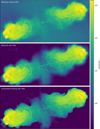 |
Fig. 1 Comparison of Cygnus A images with three algorithms. Top panel: Cygnus A image from Arras et al. (2021a) obtained with resolve without direction-dependent calibration. Central panel: the Cygnus A image reconstructed with the algorithm of this work. Bottompanel: Cygnus A image from Dabbech et al. (2021) recovered by a compressed sensing algorithm including direction-dependent calibration. The colorbar is clipped for better visibility. |
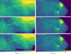 |
Fig. 2 Zooms into high and low flux regions of the reconstructions. Left column: zoom on the core and jet. Top panel: Arras et al. (2021a); central panel: this work; bottom panel: Dabbech et al. (2021). Right column: zoom on the hot spots of western lobe. Top panel: Arras et al. (2021a); central panel: this work; bottom panel: Dabbech et al. (2021). The colorbars of the left and right columns are clipped and adapted to the respective surface brightness range. |
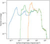 |
Fig. 3 Histogram of surface brightness values of the resolve reconstruction with direction-dependent calibration (green), the resolve reconstruction of Arras et al. (2021a) with classical calibration (orange), and the compressed sensing reconstruction from Dabbech et al. (2021) also with direction-dependent calibration (blue). The histogram is computed from the images displayed in Fig. 1 showing on the y-axis the fraction of the image with this surface brightness. |
4.4 Calibration solutions
In this section, we briefly discuss the antenna gain solutions. As our antenna gain model (3.2) factorizes the antenna gains into a purely time-dependent term ɡp(t), an only direction-dependent ɡp(l), and a jointly direction and time-dependent term ɡp(l,t), we can analyze the reconstruction of these terms separately. As it will turn out in the following sections, the statistical properties of the three factors are very different. As we model each of the factors with separate Gaussian processes, inferring their power spectra, the algorithm can capture the different statistics and exploit them to further constrain the reconstructions.
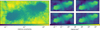 |
Fig. 4 Uncertainty quantification of the resolve reconstruction. Left column: relative uncertainty of the reconstruct sky brightness computed from posterior samples. Two right columns: four representative posterior samples of the geo VI reconstructions. |
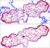 |
Fig. 5 Flux contours of the Cygnus A reconstructions. The surface brightness levels of the contours are logarithmically spaced and range from 1 mly arcsec−2 to 4.25 × 10⁴ mly arcsec−2. Top panel: in solid blue resolve reconstruction from Arras et al. (2021a) without direction-dependent calibration. In dashed red resolve reconstruction of this work with direction-dependent calibration. Bottom panel: in solid blue compressed sensing reconstruct of Dabbech et al. (2021) with direction-dependent calibration. In dashed red again resolve reconstruction of this work with direction-dependent calibration. |
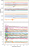 |
Fig. 6 DIE amplitude (top panel) and phase (bottom panel) of the calibration solutions for all 26 antenna in VLA configuration A. |
4.4.1 Only time-dependent gains: gp(t)
Figure 6 displays only time-dependent calibration solutions. Both the phase and the amplitude are largely stable over time, with some small-scale fluctuations. After approximately one-third of the observation, the amplitude of several antenna gains suddenly decreases before returning to the old value. The phases of the gains constantly undergo some variations.
In Fig. 7, the absolute value of the only time-dependent part of the calibration solution is depicted for one baseline, thus in formulas  To visualize the jumps in the calibration solutions discussed in the previous section, we display the absolute value of the visibilities of the flux calibrator as well as the science target Cygnus A projected to the calibration space. More precisely, we divide the visibilities of the respective observation by the model visibilities computed from the sky model without the only time-dependent calibration factor
  . Thus, as a formula,
 (16)
(16)
with Vpqt being the visibilities of the observation, C(l) the w-term correction factor, I(l) the reconstructed sky model, and
 (17)
(17)
the calibration solution excluding the only time-dependent part ɡp(t) . The offset between the visibilities from the flux calibrator and the visibilities of the Cygnus A observation is clearly visible in Fig. 7, and is on the order of a few percent. The discontinuities in the calibration solution, as described in Sect. 3.2, were introduced to model these offsets.
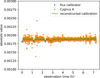 |
Fig. 7 Green: absolute value of the reconstructed time-dependent, but direction-independent, calibration for one baseline. The blue and orange dots are the absolute values of the visibilities of the flux calibrator and target observations, projected to the calibration space by dividing out their respective sky models. More specifically, blue dots: flux calibrator visibilities divided by the model visibilities computed from the flux calibrator sky model without time-dependent calibration factors. Orange dots: Cygnus A visibilities divided by the model visibilities computed from the Cygnus A sky model, including the direction-dependent calibration but excluding the purely time-dependent calibration. The offset between the calibration data points and the target data points makes it necessary to allow for possible discontinuities in the antenna gain reconstructions when switching the observation target. Partly this offset might also be due to a oversimplified flux calibrator model. |
4.4.2 Only direction-dependent gains: gp(l)
Figure 8 depicts the direction-dependent but time independent gain  of one antenna. The phase and amplitude variations are both on the level of a few percent. The interferometer is only sensitive to variations of the gain solutions in directions with significant sky surface brightness since the antenna gains are a multiplicative effect on the sky. Therefore, to indicate which regions of the reconstructed gains solutions actually affect the likelihood, we superimpose the flux contours of Cygnus A on the plot of the calibration solution.
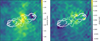 |
Fig. 8 Phase and amplitude of the direction-dependent, time-independent gain factor for one antenna. On top the flux contours of Cygnus A are indicated in white, since the interferometer is only sensitive to direction-dependent effects in regions with significant surface brightness. Thus, gain values outside the contours are neither accurate nor relevant. |
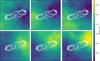 |
Fig. 9 Absolute value of jointly time and direction-dependent gain of antenna 0, depicted at six timesteps of the observation. On top, the contours of Cygnus A are shown since the interferometer is only sensitive to the direction-dependent gain variations in regions with significant sky brightness. Gain values outside the contours are neither accurate nor relevant. |
4.4.3 Jointly time and direction-dependent gains: ɡp (I, t)
The absolute value of the jointly time and direction-dependent antenna gains  from which the only time and only direction-dependent variations are excluded is displayed in Fig. 9. Similar to Fig. 8, the flux contours of Cygnus A are superimposed to indicate which regions actually have a significant effect. The variations of the jointly direction and time-dependent gains are less than a percent and therefore smaller than the only time and only direction dependent effects. The spatial correlation length is, compared to the only direction-dependent gain solutions, significantly larger. This result underlines that a split of the antenna gains into an only direction and a jointly direction and time-dependent part can be beneficiai because the generative model for
  can exploit this longer correlation length.
A direct quantitative comparison with the work of Dabbech et al. (2021), as done for the Cygnus A sky images, is not possible for the calibration solutions, as the calibration model in Dabbech et al. (2021) is different and the results are only published in the form of images. Nevertheless, the scale of the amplitude and phase variations are comparable. Also, the correlation length of the jointly direction and time-dependent gain solutions is similar to the correlation length of the direction and time-dependent calibration solutions in Dabbech et al. (2021). However, in the work of Dabbech et al. (2021), the spatial and temporal correlation lengths are set somewhat externally by specifying the support size of the corresponding Fourier kernels. In contrast, in this work, the correlation structures are not fixed but reconstructed from the data.
Pointing errors are expected to be an important source of jointly time and direction-dependent gains. The antenna beam is falling off with increasing distance to the center of the field of view. This makes the sky to appear brighter in the direction of the pointing offset and dimmer in the opposite direction, leading to a direction-dependent antenna gain. Mathematically the direction-dependent antenna gain can be computed by
 (18)
(18)
with Bp(δxt)(δyt) being the beam of antenna p with an pointing offset of (δxt, δyt), and Bp(0,0) the beam of the nominal pointing. Using Eq. (18), we fit pointing offsets to the absolute value of the direction-dependent gains, resulting in pointing offsets of up to 30arcsec as depicted in Fig. 10. As visible in Fig. 10, the gains resulting from pointing offsets relatively closely follow the reconstructed gain. Nevertheless, some deviations remain as pointing errors are not the only source for time and direction-dependent gains.
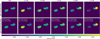 |
Fig. 10 Top row: absolute value of jointly time and direction-dependent gain of antenna 0 (same as Fig. 9) restricted to sky region with significant flux. Bottom: fit of the antenna gain resulting from pointing errors to the reconstructed gain in the top row. Except for minor differences, the gains resulting from pointing errors can reproduce the reconstructed gains. The offset fit to the nominal pointing direction is specified as δx and δy. As Cygnus A is less extended in y-direction than in x-direction, the gains are much less sensitive to pointing offsets in y-direction. |
5 Conclusions
This paper introduces a novel Bayesian radio interferometric imaging and calibration algorithm based on the resolve framework. Calibration and imaging are performed jointly. The calibration includes corrections for direction-dependent effects. To this goal, the antenna gain solutions are split into three factors, a purely time-dependent term, a purely direction-dependent term, and a jointly direction and time-dependent term. Having a separate model for each factor of the gain solutions allows one to exploit the different statistics of the individual factors.
We demonstrate the method on VLA's Cygnus A observation, a widely used target for benchmarking novel algorithms. In comparison with previous work (Arras et al. 2021a), imaging Cygnus A also with the resolve framework but classically calibrated data, the dynamic range is significantly increased. At the same time, in high and medium surface brightness regions, the two reconstructions are closely consistent. When comparing with Dabbech et al. (2021), a compressed sensing method including direction-dependent calibration, the results not only agree in high and medium surface brightness regions but also in areas with very low flux. As the reconstruction algorithms of the sky radio maps of this work and Dabbech et al. (2021) are based on very different methodologies, namely Bayesian inference and compressed sensing, their close agreement is a strong indication of their reliability even at low surface brightness regions. Furthermore, this underlines the necessity of an accurate calibration model for obtaining high-fidelity radio maps with a large dynamic range. An accurate calibration model will become a critical component for exploiting the full potential of upcoming radio interferometers.
The computational complexity of this method in its current version and the resolve framework, in general, is significantly higher compared with the clean algorithm. The higher computational costs partially arise from our inference algorithm (Sect. 3.4) computing not only a single estimate of the sky brightness but providing samples of the posterior distribution allowing for statistically robust uncertainty quantification. Additionally to the computational overhead of the posterior inference algorithm, it is in the current version of resolve necessary to always degridd to the visibility space to evaluate the likelihood. Despite fast gridding algorithms, this can, depending on the interferometer setup, lead to significantly higher computational costs compared with the clean algorithm's major/minor cycle scheme. We plan to also introduce a major/minor cycle scheme to the resolve framework for speeding up the likelihood evaluations. As doing this in a statistically sound way is nontrivial it is left for future work.
Acknowledgements
J.R. and P.A. acknowledge financial support by the German Federal Ministry of Education and Research (BMBF) under grant 05A20W01 (Verbundprojekt D-MeerKAT).
Appendix A Only DIE calibration reconstruction
For completeness, we also reconstructed Cygnus A using the same imaging and calibration setup described above, except that we removed the direction-dependent calibration terms. Thus starting from the uncalibrated data, we jointly reconstructed Cygnus A and the calibration solutions, considering only direction-independent calibration. The result of this reconstruction is depicted in Fig. A.1. Overall, the result of this reconstruction is similar to the reconstruction of Arras et al. (2021a) (displayed in Fig. 1) building on classically calibrated data.
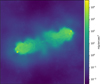 |
Fig. A.1 Cygnus A reconstruction with resolve using DIE calibration only. |
Appendix B Residual image
We computed the dirty image of the residuals between the data and our reconstruction with direction-dependent calibration. As visible in Fig. B.1, the amplitude of the residuals is very small compared with the brightness of Cygnus A. Nearly no structures of the source have imprinted on the residual image, indicating that the reconstructed sky model and antenna gains model the data very well. The only structures of Cygnus A of which some remnants can be found in the residual image are the hot spots of the lobes and the jet. Interestingly remnants of the jet are not only visible at the actual position of the jet but also at various shifted positions. We believe this originates from the nature of our prior model for diffuse emission. As outlined in Sect. 3.1.1, we model the diffuse emission with a Gaussian process represented in Fourier space. The Fourier mode corresponding to the width and orientation of the jet should be strongly exited, leading to an oscillation with this width and orientation in the entire field of view. Nevertheless, the amplitude of this effect is very small compared to the brightness of Cygnus A and its jet. Therefore, this oscillatory effect cannot be seen in the reconstructions (Fig. 1).
Dabbech et al. (2021) reported the detection of three additional sources in the residual image further away from Cygnus A. We cannot confirm these sources as they are not found in our residual image.
 |
Fig. B.1 Dirty image of the residuals between our reconstruction and the actual data. |
References
- Albert, J. G., van Weeren, R. J., Intema, H. T., & Röttgering, H. J. A. 2020, A & A, 635, A147 [CrossRef] [EDP Sciences] [Google Scholar]
- Arras, P., Frank, P., Leike, R., Westermann, R., & Enßlin, T. A. 2019, A & A, 627, A134 [NASA ADS] [CrossRef] [EDP Sciences] [Google Scholar]
- Arras, P., Bester, H. L., Perley, R. A., et al. 2021a, A & A, 646, A84 [NASA ADS] [CrossRef] [EDP Sciences] [Google Scholar]
- Arras, P., Martin, R., Westermann, R., & Enßlin, T. A. 2021b, A & A, 646, A58 [NASA ADS] [CrossRef] [EDP Sciences] [Google Scholar]
- Arras, P., Frank, P., Haim, P., et al. 2022, Nat. Astron., 6, 259 [NASA ADS] [CrossRef] [Google Scholar]
- Bhatnagar, S., Cornwell, T. J., Golap, K., & Uson, J. M. 2008, A & A, 487, 419 [NASA ADS] [CrossRef] [EDP Sciences] [Google Scholar]
- Birdi, J., Repetti, A., & Wiaux, Y. 2020, MNRAS, 492, 3509 [Google Scholar]
- Cornwell, T. J., & Perley, R. A. 1992, A & A, 261, 353 [NASA ADS] [Google Scholar]
- Cornwell, T. J., Golap, K., & Bhatnagar, S. 2008, IEEE J. Selected Top. Signal Process., 2, 647 [NASA ADS] [CrossRef] [Google Scholar]
- Dabbech, A., Onose, A., Abdulaziz, A., et al. 2018, MNRAS, 476, 2853 [Google Scholar]
- Dabbech, A., Repetti, A., & Wiaux, Y. 2019, in International BASP Frontiers Workshop 2019, 23 [Google Scholar]
- Dabbech, A., Repetti, A., Perley, R. A., Smirnov, O. M., & Wiaux, Y. 2021, MNRAS, 506, 4855 [NASA ADS] [CrossRef] [Google Scholar]
- Enßlin, T. A. 2019, Ann. Phys., 531, 1800127 [Google Scholar]
- Frank, P., Leike, R., & Enßlin, T. A. 2021, Entropy, 23 [Google Scholar]
- Guardiani, M., Frank, P., Kostic, A., et al. 2022, PLoS One, 17, e0275011 [NASA ADS] [CrossRef] [Google Scholar]
- Khintchine, A. 1934, Math. Ann., 109, 604 [CrossRef] [Google Scholar]
- Knollmüller, J., & Enßlin, T. A. 2018, ArXiv e-prints [arXiv:1812.84483] [Google Scholar]
- Offringa, A. R., McKinley, B., Hurley-Walker, N., et al. 2014, MNRAS, 444, 606 [Google Scholar]
- Perley, R. A. 1999, in ASP Conf. Ser., 180, Synthesis Imaging in Radio Astronomy II, 383 [Google Scholar]
- Perley, R. A., & Butler, B. J. 2013, ApJS, 204, 19 [Google Scholar]
- Pratley, L., Johnston-Hollitt, M., & McEwen, J. D. 2019, ApJ, 874, 174 [NASA ADS] [CrossRef] [Google Scholar]
- Repetti, A., Birdi, J., Dabbech, A., & Wiaux, Y. 2017, MNRAS, 470, 3981 [Google Scholar]
- Sebokolodi, M. L. L., Perley, R., Eilek, J., et al. 2020, ApJ, 903, 36 [NASA ADS] [CrossRef] [Google Scholar]
- Selig, M., Vacca, V., Oppermann, N., & Enßlin, T. A. 2015, A & A, 581, A126 [NASA ADS] [CrossRef] [EDP Sciences] [Google Scholar]
- Smirnov, O. M. 2011, A & A, 527, A106 [NASA ADS] [CrossRef] [EDP Sciences] [Google Scholar]
- Smirnov, O. M., & Tasse, C. 2015, MNRAS, 449, 2668 [Google Scholar]
- Tasse, C., Hugo, B., Mirmont, M., et al. 2018, A & A, 611, A87 [NASA ADS] [CrossRef] [EDP Sciences] [Google Scholar]
- Thouvenin, P.-A., Repetti, A., Dabbech, A., & Wiaux, Y. 2018, in 2018 IEEE 10th Sensor Array and Multichannel Signal Processing Workshop (SAM), 475 [CrossRef] [Google Scholar]
- van der Tol, S., Veenboer, B., & Offringa, A. R. 2018, A & A, 616, A27 [NASA ADS] [CrossRef] [EDP Sciences] [Google Scholar]
- van Weeren, R. J., Williams, W. L., Hardcastle, M. J., et al. 2016, ApJS, 223, 2 [Google Scholar]
- Ye, H., Gull, S. F., Tan, S. M., & Nikolic, B. 2021, MNRAS, 510, 4110 [Google Scholar]
All Figures
|
Fig. 1 Comparison of Cygnus A images with three algorithms. Top panel: Cygnus A image from Arras et al. (2021a) obtained with resolve without direction-dependent calibration. Central panel: the Cygnus A image reconstructed with the algorithm of this work. Bottompanel: Cygnus A image from Dabbech et al. (2021) recovered by a compressed sensing algorithm including direction-dependent calibration. The colorbar is clipped for better visibility. |
| In the text | |
|
Fig. 2 Zooms into high and low flux regions of the reconstructions. Left column: zoom on the core and jet. Top panel: Arras et al. (2021a); central panel: this work; bottom panel: Dabbech et al. (2021). Right column: zoom on the hot spots of western lobe. Top panel: Arras et al. (2021a); central panel: this work; bottom panel: Dabbech et al. (2021). The colorbars of the left and right columns are clipped and adapted to the respective surface brightness range. |
| In the text | |
|
Fig. 3 Histogram of surface brightness values of the resolve reconstruction with direction-dependent calibration (green), the resolve reconstruction of Arras et al. (2021a) with classical calibration (orange), and the compressed sensing reconstruction from Dabbech et al. (2021) also with direction-dependent calibration (blue). The histogram is computed from the images displayed in Fig. 1 showing on the y-axis the fraction of the image with this surface brightness. |
| In the text | |
|
Fig. 4 Uncertainty quantification of the resolve reconstruction. Left column: relative uncertainty of the reconstruct sky brightness computed from posterior samples. Two right columns: four representative posterior samples of the geo VI reconstructions. |
| In the text | |
|
Fig. 5 Flux contours of the Cygnus A reconstructions. The surface brightness levels of the contours are logarithmically spaced and range from 1 mly arcsec−2 to 4.25 × 10⁴ mly arcsec−2. Top panel: in solid blue resolve reconstruction from Arras et al. (2021a) without direction-dependent calibration. In dashed red resolve reconstruction of this work with direction-dependent calibration. Bottom panel: in solid blue compressed sensing reconstruct of Dabbech et al. (2021) with direction-dependent calibration. In dashed red again resolve reconstruction of this work with direction-dependent calibration. |
| In the text | |
|
Fig. 6 DIE amplitude (top panel) and phase (bottom panel) of the calibration solutions for all 26 antenna in VLA configuration A. |
| In the text | |
|
Fig. 7 Green: absolute value of the reconstructed time-dependent, but direction-independent, calibration for one baseline. The blue and orange dots are the absolute values of the visibilities of the flux calibrator and target observations, projected to the calibration space by dividing out their respective sky models. More specifically, blue dots: flux calibrator visibilities divided by the model visibilities computed from the flux calibrator sky model without time-dependent calibration factors. Orange dots: Cygnus A visibilities divided by the model visibilities computed from the Cygnus A sky model, including the direction-dependent calibration but excluding the purely time-dependent calibration. The offset between the calibration data points and the target data points makes it necessary to allow for possible discontinuities in the antenna gain reconstructions when switching the observation target. Partly this offset might also be due to a oversimplified flux calibrator model. |
| In the text | |
|
Fig. 8 Phase and amplitude of the direction-dependent, time-independent gain factor for one antenna. On top the flux contours of Cygnus A are indicated in white, since the interferometer is only sensitive to direction-dependent effects in regions with significant surface brightness. Thus, gain values outside the contours are neither accurate nor relevant. |
| In the text | |
|
Fig. 9 Absolute value of jointly time and direction-dependent gain of antenna 0, depicted at six timesteps of the observation. On top, the contours of Cygnus A are shown since the interferometer is only sensitive to the direction-dependent gain variations in regions with significant sky brightness. Gain values outside the contours are neither accurate nor relevant. |
| In the text | |
|
Fig. 10 Top row: absolute value of jointly time and direction-dependent gain of antenna 0 (same as Fig. 9) restricted to sky region with significant flux. Bottom: fit of the antenna gain resulting from pointing errors to the reconstructed gain in the top row. Except for minor differences, the gains resulting from pointing errors can reproduce the reconstructed gains. The offset fit to the nominal pointing direction is specified as δx and δy. As Cygnus A is less extended in y-direction than in x-direction, the gains are much less sensitive to pointing offsets in y-direction. |
| In the text | |
|
Fig. A.1 Cygnus A reconstruction with resolve using DIE calibration only. |
| In the text | |
|
Fig. B.1 Dirty image of the residuals between our reconstruction and the actual data. |
| In the text | |
Current usage metrics show cumulative count of Article Views (full-text article views including HTML views, PDF and ePub downloads, according to the available data) and Abstracts Views on Vision4Press platform.
Data correspond to usage on the plateform after 2015. The current usage metrics is available 48-96 hours after online publication and is updated daily on week days.
Initial download of the metrics may take a while.