| Issue |
A&A
Volume 668, December 2022
|
|
|---|---|---|
| Article Number | A127 | |
| Number of page(s) | 11 | |
| Section | Interstellar and circumstellar matter | |
| DOI | https://doi.org/10.1051/0004-6361/202244621 | |
| Published online | 16 December 2022 | |
The l = 2 spherical harmonic expansion coefficients of the sky brightness distribution between 0.5 and 7 MHz
1
Space Sciences Laboratory, University of California,
Berkeley, CA
94720, USA
e-mail: This email address is being protected from spambots. You need JavaScript enabled to view it.
2
Department of Physics, University of California,
Berkeley, CA
94720, USA
3
Center for Astrophysics and Space Astronomy, University of Colorado,
Boulder, CO
80309, USA
4
Department of Astrophysical and Planetary Sciences, University of Colorado,
Boulder, CO
80309, USA
5
LESIA, Observatoire de Paris, PSL Université, CNRS, Sorbonne Université, Université de Paris,
92195
Meudon, France
6
NASA Ames Research Center,
Moffett Field, CA
94035, USA
7
Research Institute for Advanced Computer Science, Universities Space Research Association,
Washington, DC
20024, USA
Received:
28
July
2022
Accepted:
28
October
2022
Abstract
Context. The opacity of the ionosphere prevents comprehensive Earth-based surveys of low frequency ν ≲ 10 MHz astrophysical radio emissions. The limited available data in this frequency regime show a downturn in the mean sky brightness at ν ≲ 3 MHz in a divergence from the synchrotron emission power-law that is observed at higher frequencies. The turning over of the spectrum coincides with a shift in the region of maximum brightness from the Galactic plane to the poles. This implicates free-free absorption by interstellar ionized gas, whose concentration in the plane causes radiation that propagates in this region to suffer stronger absorption than radiation from the poles.
Aims. Using observations from Parker Solar Probe (PSP), we evaluate the l = 0 and l = 2 spherical harmonic expansion coefficients of the radio brightness distribution at 56 frequencies between 0.5 and 7 MHz. These data quantify free-free absorption’s global effects on the brightness distribution, which provides new constraints on the distribution of free electrons in the Galaxy.
Methods. The auto and cross spectra of the voltages induced on crossed short dipole antennas by radiation from a nonpolarized extended brightness distribution are linear combinations of the distribution’s l = 0 and l = 2 expansion coefficients. We extracted the least squares solution to these coefficients from PSP’s measurements of the radio background. Also, we generated hypothetical low frequency brightness maps that incorporated free-free absorption and tested their compatibility with the data. The maps primarily depended on models of the Galactic emissivity and distribution of free electrons. A comparison of the maps’ expansion coefficients with the empirical coefficients provided an indication of these input models’ accuracies.
Results. An average reduced x2 ≈ 1.04 of the spherical harmonic analysis between 0.5 and 7 MHz indicates that PSP’s antennas act approximately as ideal short dipoles in this frequency band. The best-fit expansion coefficients show that, with decreasing frequency, the mean sky brightness decreases at ν < 3 MHz and the Galactic plane darkens relative to the poles. At ν > 0.6 MHz, these observations can be reproduced in synthetic brightness maps in which the Galactic emissivity maintains a power-law form and free-free absorption is modeled using free electron distributions derived from pulsar measurements. At lower frequencies, the empirical mean brightness falls below the mean in this model, possibly signifying a cutoff in the synchrotron power-law.
Key words: radio continuum: ISM / Galaxy: disk / opacity / methods: data analysis
© B. Page et al. 2022
 Open Access article, published by EDP Sciences, under the terms of the Creative Commons Attribution License (https://creativecommons.org/licenses/by/4.0), which permits unrestricted use, distribution, and reproduction in any medium, provided the original work is properly cited.
This article is published in open access under the Subscribe-to-Open model. This email address is being protected from spambots. You need JavaScript enabled to view it. to support open access publication.
1 Introduction
Free-free absorption by ionized hydrogen in the Galaxy causes the low frequency (ν ≲ 10 MHz) Galactic radio spectrum to deviate from the power-law that is observed at higher frequencies (e.g., Verschuur & Kellermann 1988, p. 10). Early evidence for this came from an analysis of the variation in the ratio of the flux at 18.3 MHz to that at 100 MHz as a function of Galactic latitude (Shain 1954). The ratio achieves a minimum in the Galactic plane, and its trend in latitude is consistent with a decrease in path length through some absorbing material as the line of sight becomes elevated above it. Modeled as a spatially uniform disk of height h that extends from the Galactic center to at least the position of the Earth, the material could be assessed to have an absorption coefficient α(ν = 1 MHz) = 14/h. Under the hypothesis of free-free absorption by ionized hydrogen, this result can be used with the theoretical expression
 (1)
(1)
to constrain the parameters of the disk gas (Verschuur & Kellermann 1988, p. 41). Here, Te is the electron temperature and ne is the electron density. One possible set of parameters satisfying α(ν = 1 MHz) × h = 14 is a height on the order of a few hundred parsecs, a density ne ≈ 0.1−1 cm−3, and a temperature Te ≈ 104 K.
Reber & Ellis (1956) developed methods for controlling ground-based observations at ν < 10 MHz for ionospheric attenuation and terrestrial interference, allowing for measurements of the radio background from 1.5 to 9.8 MHz to be obtained. These revealed that free-free absorption becomes strong enough to cause the background’s average intensity to peak at a few megahertz and subsequently decrease with decreasing frequency (Ellis et al. 1962). The angular resolution of the measurements was limited to a few steradians, but still a difference in behavior could be detected between the flux from the plane and that from the poles. Spectra collected from both regions featured a downturn, but a slightly greater frequency of peak brightness in spectra from the plane indicated stronger absorption there. A disk model for the responsible gas was therefore adopted once more, with a height h = 300 pc, temperature Te = 104 K, and density ne = 0.1 cm−3 found to be compatible with the measurements (Hoyle & Ellis 1963).
Later space-based observations from the Radio Astronomy Explorer-I spacecraft (RAE-I) between 0.4 and 6.5 MHz confirmed the presence of a peak in the mean brightness near 3 MHz (Alexander et al. 1970). These measurements also revealed that, at the few steradian resolution of RAE-I’s antennas, the Galactic poles become brighter than the Galactic plane at about 2 MHz. Higher resolution maps later constructed by Ellis (1982) showed that a minimum in brightness in fact occurs at the Galactic center at 2 MHz. A uniform disk of absorbing material could no longer explain these observations, which instead demonstrated a positive spatial correlation of absorptivity and emissivity at low frequencies that causes the high frequency brightness distribution to become inverted. More recently, a study using the dipole measurements from the Wind spacecraft again found a shift in the region of maximum brightness from the plane to the poles at a few megahertz (Manning & Dulk 2001).
Lecacheux & Maksimovic (2019) established that the information about the sky brightness distribution that can be extracted from measurements by colocated dipole antennas is restricted to the distribution’s l = 0 and l = 2 spherical harmonic expansion coefficients. They obtained approximate values for the coefficients at 1.5 MHz using data from the Cassini spacecraft that showed the flux from the Galactic poles to be stronger than that from the plane. We used measurements from Parker Solar Probe (PSP) to determine the l = 2 coefficients between 0.5 and 7 MHz, which depict the evolution of the brightness distribution to this state of relatively diminished plane flux.
To assess the compatibility of the l = 0 and l = 2 coefficients with free-free absorption effects, we employed a model of the distribution of free electrons in the Galaxy that was principally derived from observations of pulsar signal dispersion and broadening (e.g., Manchester & Taylor 1981; Taylor & Cordes 1993; Cordes & Lazio 2002; Yao et al. 2017). An early set of pulsar data conformed to a distribution consisting of two axially symmetric components, one with a scale height of 70 pc and scale radius 10 kpc and the other extending to all heights with the same radial profile (Manchester & Taylor 1981). After iteration over several decades, the model distributions now additionally include spiral arms, discrete features within 1 kpc of the Earth such as Loop I (Taylor & Cordes 1993; Cordes & Lazio 2002), and refinements such as an offset in the position of the Solar System from the Galactic plane and a warp in one of the disks (Yao et al. 2017).
Under some simplifying assumptions, these models allow for calculation of the free-free optical depth to any location in the Galaxy. In conjunction with an emissivity model, this enables the generation of synthetic brightness maps at low frequencies (Cong et al. 2021). We produced such maps and compared their l = 0 and l = 2 expansion coefficients to the measured coefficients. For the Galactic emissivity, we employed a fit to the Haslam et al. (1982) 408 MHz survey and assumed a power-law dependence on frequency with spectral index β ≈ −2.5. To assess optical depth, we utilized the free electron distribution of Yao et al. (2017) and information about turbulent density fluctuations from Cordes & Lazio (2002).
Our main result is the empirical set of spherical harmonic coefficients, and we only present broad conclusions from them about the Galactic emissivity and distribution of free electrons. Bassett et al.(in prep.) plan to analyze the PSP data with a greater focus on constraining the physical parameters of the Galaxy.
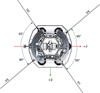 |
Fig. 1 Antenna system of PSP. The four sensors V1, V2, V3, and V4 are mounted to and coplanar with the spacecraft heat shield, which is located in the back of the diagram. Radiator fins extend from the heat shield to a 1.5 m long hexagonal spacecraft bus in the foreground. The |


2 Data
2.1 Instrument
Measurements of the Galactic radio background are made by the Radio Frequency Spectrometer (RFS) component of the FIELDS instrument suite on PSP (Bale et al. 2016; Pulupa et al. 2017). The electric field antenna of FIELDS is composed of two crossed dipole antennas, each of which is made up of a collinear pair of the sensors V1, V2, V3, and V4 shown in Fig. 1. The tip-to-tip length of the V1–V2 dipole is 6.975 m and that of the V3–V4 dipole is 6.889 m. Each individual sensor consists of a 1/8″ diameter, 2 m long tubular “whip” attached to a collinear 30 cm long tubular “stub” that mounts to the spacecraft heat shield. A wire enclosed in the stub carries signals from the whip to a coaxial cable that connects to a preamplifier near the sensor’s mounting point.
In the frequency band of our results, the measured voltages V = GVoc differ from the open-circuit antenna voltage Voc by a gain factor G = Ca/(Ca + Cs) due to, in each sensor’s signal path, “stray” capacitance Cs in series with the intrinsic capacitance Ca of the sensor (Pulupa et al. 2017). Lab measurements carried out on a model sensor assembly indicate that Cs = 36 pF and Ca = 17 pF. This value for Ca is similar to the theoretical expectation for a monopole of length 2 m and diameter 1/8″ above an infinite ground plane. A few capacitive paths in the circuit that contribute to Cs are that from whip to stub to ground and that between the center and shield conductors in the coaxial cable. The resulting gain G = 0.32 is the best current estimate and differs from the value given in Pulupa et al. (2017) due to revisions in the estimates for Cs and Ca.
Our analysis depended on accurate knowledge of the pointing directions of the antennas. In the spacecraft coordinate system, they are aligned as illustrated in Fig. 1 within a margin of 1° .In turn, the orientation of PSP in space is measured to 0.1° accuracy (Fox et al. 2015). To interface with the PSP attitude data, we used the SPICE toolkit provided by NASA (Acton et al. 2018).
2.2 Digital signal processing
The RFS digitizes two input signals at a rate of 38.4 MHz and computes estimates of their auto and cross spectral densities (Pulupa et al. 2017). The estimates are made both in a high frequency band (HFR) from 0 to 19.2 MHz and, after the data are downsampled to an effective 4.8 MHz sampling rate, in a low frequency band (LFR) from 0 to 2.4 MHz. The spectra in both bands are composed of 2048 frequency bins, giving spacings Δν = 9375 Hz in the HFR and Δν = 1171.875 Hz in the LFR.
Prior to telemetry to ground, the spectra are averaged over frequency and time to decrease their standard errors. Also, their frequency coverage is reduced to a selection of bins intended to capture the most scientifically valuable information in each spectrum while allowing for a greater quantity of spectra in the RFS’s telemetry budget. Specifically, reduced LFR spectra are comprised of averages over three adjacent full spectrum frequency bins at 64 logarithmically spaced center frequencies between 10 kHz and 1.7 MHz. Reduced HFR spectra are constructed in the same way with center frequencies between 1.3 and 19.2 MHz. Under the RFS’s current default settings and in the absence of signals that overrange the instrument, the spectra are averaged in time over 80 spectra. Again in the case of no overranges, which applies to all measurements that we use, these 80 spectra are captured in a time span of approximately 2 s.
The data available for analysis are these time-averaged reduced spectra. To be specific, the summing operations of the averaging take place on the spacecraft, and on-ground conversion to units of power spectral density includes division by the number of summands at each data point, which is 3 × 80 = 240 in this study.
We use measurements of the cross  and the auto
  and
and  spectra of the two dipole voltages V12 and V34. For the standard error on the auto spectra we adopt
  . As expected from a Galactic background that is unpolarized at the resolution of dipole antennas, the cross spectrum is purely real. We therefore use for its standard error
  (Brillinger 2001, p. 237).
2.3 Noise
Figure 2 shows the amplitude of the Galactic background relative to the amplitudes of the two dominant noise sources in the RFS measurements. Thermal electronic noise arises primarily from the preamplifier and analog filtering stages of the RFS signal chain. At frequencies above ~1 MHz, its amplitude is approximately 20 nV2/Hz in the dipole auto spectra that we analyzed, which is similar to the spectral power from the Galaxy. The intensity of the Galactic background decreases with decreasing frequency and it is exceeded by the electronic noise power by a factor of 10 at 500 kHz.
Preflight bench tests indicate that, at 298 K, the two preamps in a dipole measurement each contribute noise of form (7.4 + 0.38 (ν/1 MHz)−2) nV2/Hz and the analog filtering electronics contribute 6.0 nV2/Hz of frequency-independent noise. We scaled the 298 K noise power of the components by their temperatures in space, which were measured by a thermistor on each of the preamps and on the FIELDS Data Control Board, where the analog electronics are located. We then subtracted from each auto spectrum the scaled noise of its two input preamps and the analog electronics. Ideally, this noise is rejected in the cross spectrum due to independence of the thermal electronic fluctuations in the two dipole signals.
Noise also arises from electron motion in the vicinity of the antennas (e.g., Meyer-Vernet 1979; Moncuquet et al. 2020). This so-called quasi-thermal noise (QTN) depends on the time-varying ambient electron density and temperature and so could not be mitigated as easily as the electronic noise. We used measurements captured at about 0.8 au from the Sun and found that the QTN was well approximated in the auto spectra by a power-law A(v/ 1 MHz)−b at frequencies ν ≫ vpe with A around 10 nV2 / Hz and b around 1.5. Here, vpe is the electron plasma frequency and is typically about 30 kHz at 0.8 au. With the electronic noise removed, we fit for A and b between 300 and 400 kHz, where the QTN was stronger than the Galaxy signal by several orders of magnitude, and subtracted out the resulting power-law from the auto spectra. Because the two dipoles are not exactly orthogonal, the QTN was expected to be present in the cross spectra as well, but at a level suppressed by a factor of about 100 compared to that in the auto spectra (Meyer-Vernet 1979).
This data cleaning procedure left a discrepancy between the V1–V2 and V3–V4 signals at ν > 3 MHz, the magnitude of which is indicated by the error bars in Fig. 2. This was likely caused by antenna-dependent deviations of the signal chain noise from the idealized functional form to which we fit it. Such defects were evident in the preflight bench data. We did not attempt to correct for them because their temperature dependence was unknown and they did not have exactly the same form in flight as on the bench. The resulting ≈5% uncertainty on the Galactic background at ν > 3 MHz did not impact our analysis. At lower frequencies, the error bars are dominated by the statistical uncertainty mentioned in Sect. 2.2.
The l = 2 spherical harmonic analysis only depended on the variation of the measured power with antenna orientation, so noise that was constant in time did not affect it. Furthermore, noise fluctuations with characteristic time scales longer than the 24 minute period discussed in Sect. 3.2 could be removed with a rolling average. Faster fluctuations with amplitudes non-negligible compared to the power variation due to the sky anisotropy had the potential to corrupt the analysis. Across the band where we extracted the l = 2 coefficients from 0.5 to 7 MHz, the amplitude of the sky anisotropy signal ranged from 0.5 to 2 nV2/Hz. We found that variation in the QTN in the auto spectra was comparable to this at frequencies below ≈1.8 MHz, so we only used the cross spectra in this range. At frequencies v < 0.5 MHz, QTN oscillations impacted the cross spectra as well, preventing extraction of the spherical harmonic coefficients.
Lastly, in the measurements that we considered, bursts of radiation from Jupiter and the Sun respectively had peak flux densities similar to and several times higher than the Galactic background. We identified time spans that included these emissions by visual inspection and omitted them in our analysis of the Galaxy. Stretches of data that we excised are recorded in Table 1.
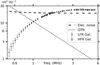 |
Fig. 2 Amplitudes of the Galactic background, thermal electronic noise, and quasi-thermal noise in the RFS auto spectra. |
Roll maneuver data sets.
3 Dipole antenna measurements of an unpolarized extended brightness distribution
3.1 Spherical harmonic decomposition
The sky is taken to consist of unpolarized radiation with specific intensity B(k, ν) a function of the line of sight k and frequency v. In a coordinate system with its z-axis along k, the contribution to the electric field spectral density matrix 〈E(v)E†(v)〉 from a patch of sky dΩ centered on k is given by
![Mathematical equation: $d\left\langle {{\bf{E}}\left( v \right){{\bf{E}}^\dag }\left( v \right)} \right\rangle = {{{Z_0}B\left( {k,v} \right)} \over 2}\left[ {\matrix{1 \hfill & 0 \hfill & 0 \hfill \cr 0 \hfill & 1 \hfill & 0 \hfill \cr 0 \hfill & 0 \hfill & 0 \hfill \cr} } \right]{\rm{d\Omega }} = {{\rm{\Gamma }}_E}\left( {k,v} \right){\rm{d\Omega }}$](/articles/aa/full_html/2022/12/aa44621-22/aa44621-22-eq10.png) (2)
(2)
where Z0 is the impedance of free space and the factor of 1/2 results from averaging over all linear polarizations.
The open-circuit voltage Voc(v) produced across the terminals of an antenna with height vector h(k, v) by the electric field E(k, v) of a wave from direction k with frequency v is
 (3)
(3)
where † indicates Hermitian conjugation. In general, h(k, v) is complex and depends on k and v, but for a short ideal dipole is simply a real vector parallel to the physical antenna, independent of k and v (e.g., Balanis 1992). Short here means that the antenna length is much smaller than the radiation wavelength, which is true of PSP’s antennas at v ≪ 100 MHz.
The voltage spectral density matrix corresponding to ΓE (k, v) for some system of antennas is given by
 (4)
(4)
where H is a matrix whose columns are the antenna height vectors. The following analysis requires that H be independent of k, although H is not restricted to being real.
To integrate Eq. (4) over the sky, it is convenient to express H in some fixed working coordinate system and introduce transformations R(k) to a coordinate system with its z-axis along k. The elements of the R matrices consist of trigonometric terms whose arguments determine the coordinate system transformation. For example, if k has azimuthal angle φ and polar angle θ in the working coordinate system, then R(k) = (Rz(φ)Ry(θ))⊤, where Rz and Ry are rotations about z and y.
As a result, integration of ΓV(k, v) over the sky projects out expansion coefficients, bl,m(v), that multiply spherical harmonics,  , in the decomposition
  (Lecacheux & Maksimovic 2019). Specifically, the matrix of voltage spectral densities is given by
 (5)
(5)
 (6)
(6)
where
![Mathematical equation: ${C_{4\pi }} \equiv \sqrt {{{2\pi } \over {15}}} \left[ {\matrix{{{{2\sqrt 5 {b_{0,0}} + {b_{2,0}}} \over {\sqrt 6 }} - {\rm{Re}}\left( {{b_{2,2}}} \right)} & {{\rm{Im}}\left( {{b_{2,2}}} \right)} & {{\rm{Re}}\left( {{b_{2,1}}} \right)} \cr {{\rm{Im}}\left( {{b_{2,2}}} \right)} & {{{2\sqrt 5 {b_{0,0}} + {b_{2,0}}} \over {\sqrt 6 }} - {\rm{Re}}\left( {{b_{2,2}}} \right)} & { - {\rm{Im}}\left( {{b_{2,1}}} \right)} \cr {{\rm{Re}}\left( {{b_{2,1}}} \right)} & { - {\rm{Im}}\left( {{b_{2,1}}} \right)} & {{{2\sqrt 5 {b_{0,0}} + {b_{2,0}}} \over {\sqrt 6 }}} \cr} } \right].$](/articles/aa/full_html/2022/12/aa44621-22/aa44621-22-eq17.png) (7)
(7)
Equation (6) indicates that in the short dipole case of real H, the cross spectrum is also purely real. We did not find a signal from the Galaxy in the imaginary part of the cross spectrum measured by PSP, so we restricted our analysis to real H. In full, the PSP data were fit to
![Mathematical equation: $\left[ {\matrix{{\left\langle {{V_{12}}V_{12}^*} \right\rangle } & {\left\langle {{V_{12}}V_{34}^*} \right\rangle } \cr {\left\langle {{V_{34}}V_{12}^*} \right\rangle } & {\left\langle {{V_{34}}V_{34}^*} \right\rangle } \cr} } \right] = {G^2}{Z_0}{H^{\rm{T}}}{C_{4\pi }}H$](/articles/aa/full_html/2022/12/aa44621-22/aa44621-22-eq18.png) (8)
(8)
where G is the capacitive gain factor described in Sect. 2.1.
3.2 Method for extracting the spherical harmonic expansion coefficients
For real antenna vectors h and d,
 (9)
(9)
with
![Mathematical equation: ${F_{0,hd}} \equiv \sqrt {{\pi \over {45}}} \left[ {2\sqrt 5 \left( {{\bf{h}} \cdot {\bf{d}}} \right){b_{0,0}} + \left( {{\bf{h}} \cdot {\bf{d}} - 3{h_z}{d_z}} \right){b_{2,0}}} \right],$](/articles/aa/full_html/2022/12/aa44621-22/aa44621-22-eq20.png) (10)
(10)
 (11)
(11)
 (12)
(12)
where h⊥ ≡ hx + ihy and d⊥ ≡ dx + idy. From the auto (h = d) and cross (h ≠ d) spectra measured by PSP’s crossed dipoles in some given orientation, Eq. (9) provides three linear equations for the six unknowns b0,0, b2,0, Re(b2,1), Im(b2,1), Re(b2,2), and Im(b2,2). If the antennas are then reoriented on the sky and three more independent equations are acquired, then the expansion coefficients are in principal fully determined. However, this procedure was made deficient by the presence of noise.
In the auto spectra, the combined amplitude of the signal chain and quasi-thermal noise exceeded the sky anisotropy signal by an order of magnitude, so a small fractional error in the noise’s removal significantly distorted the solution for the b2,m. Changes in the residual noise both across time and between the various auto and cross spectra impacted the analysis. To mitigate the latter changes, we first separately considered the variations of  ,
,  , and
, and  with antenna orientation and later combined the observations while ignoring the spectra’s average levels.
This was made convenient by PSP’s execution of so-called coning roll maneuvers. When at a heliocentric distance of about 0.8 au, with its z-axis pointing 45° from and its y-axis perpendicular to the Sun-pointing direction, PSP rotates about a line directed from its rear to the Sun at a rate of one rotation every 24 min. In a fixed coordinate system with its z-axis along the roll axis, h⊥ and d⊥ evolve as h⊥ → h⊥eiΩt and d⊥ → d⊥eiΩt, where Ω is the roll angular frequency. The Fn,hd are then Fourier coefficients of the resulting variation in the spectra at n times the roll frequency.
From the Fourier coefficients of the time series of each spectrum, Eq. (11) provides an estimate of b2,1 and Eq. (12) an estimate of b2,2. In the absence of noise, b0,0 and b2,0 can be determined from the F0,hd of pairs of spectra using Eq. (10). Alternatively, a solution for b2,0 can be found from the results of a second roll maneuver that has a different roll axis. Specifically, if expansion coefficient solutions  and
and  for this second coordinate system are extracted, it is known that they are related to the coefficients in the first as
  , which allows b2,0 of the first coordinate system to be determined. Here, D(2)(R) is the l = 2 Wigner D-matrix for the transformation R between the coordinate systems, and the fact that the sky brightness distribution is pure real requires that
  , with the superscript * denoting complex conjugation.
We were able to further mitigate the noise by excluding the auto spectra entirely. The results that we present at frequencies v < 1.8 MHz were acquired using just the cross spectrum n = 1 and n = 2 Fourier coefficients. For each of the five roll maneuvers listed in Table 1 and in each spectral frequency bin, these coefficients gave four real equations determining b2,1 and b2,2 in the roll coordinate system. In each bin, we compiled these into a system of 20 equations for the five unknowns b2,0, Re(b2,1) , Im(b2,1), Re(b2,2), and Im(b2,2) of the Galactic coordinate system and extracted the least squares solution. At higher frequencies, the QTN was not as strong in the auto spectra, so their F1 and F2 coefficients could also be used. From the same five roll maneuvers, this resulted in a system of 60 equations for the unknowns.
4 Results
4.1 Average spectrum
The mean sky brightness presented in Figs. 2 and 3 was derived from the average value of the noise-corrected auto spectra during the rolls. Equation (10) shows that the  anisotropic brightness is present in the roll average. We used the solution for b2,0 from the fluctuating part of the spectra to remove this contribution, leaving only the isotropic component b0,0. This correction changed the roll average only by a few percent at all frequencies. The noise-free, roll-averaged, and anisotropy-corrected auto spectra,
  and
and  , are related to the mean brightness
  as
as
 (13)
(13)
where L is the effective length of the relevant antenna, 8π/3 is the dipole beam size, and an additional factor of 1/2 results from averaging over linear polarizations (Zaslavsky et al. 2011). A comparison of the  indicated that the ratio of the V3–V4 to the V1–V2 effective length L34/L12 = 0.99 ± 0.01. This left
  unknown to an overall scaling factor, for example one of the antenna lengths.
To determine the overall scaling, we used the measurements of Novaco & Brown (1978) from the RAE-II spacecraft shown in Fig. 3. These consist of values for the flux from regions of the sky near the Galactic center, anticenter, and poles. We compared them with  from PSP under the hypothesis that their scatter about the full sky mean averaged to zero. Specifically, we computed the L2 that minimized
 (14)
(14)
with B(v) given by the RAE-II data and where the PSP data were evaluated at the RAE-II frequencies using an interpolation that was linear in log(v) and  . We only used measurements at v > 1 MHz, where the QTN was weaker than the Galaxy signal in the PSP spectra.
The solution L12 = 3.3 ± 0.1 m and L34/L12 = 0.99 ± 0.01 yields the PSP flux measurements shown in Fig. 3. There is good agreement with the Novaco & Brown (1978) data at v ≳ 0.7 MHz. At lower frequencies, the PSP mean intensity is less than that measured by RAE-II and other prior instruments (e.g., Brown 1973), which is likely caused by the small signal to noise ratio here in the PSP measurements. For this reason, we defer to the results from Novaco & Brown (1978) at ν < 0.7 MHz.
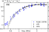 |
Fig. 3 Mean sky intensity measurements from PSP scaled to data from Novaco & Brown (1978) using effective antenna lengths, L12 = 3.3 ± 0.1 m and L34/L12 = 0.99 ± 0.01, that minimize the summed squared residuals between the data sets. The relative uncertainty on most of the Novaco & Brown (1978) points is between 15 and 20%. |
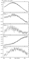 |
Fig. 4 Spherical harmonic expansion coefficients of the radio brightness distribution between 0.5 and 7 MHz. Section 4.3 describes the sources of uncertainty in the results. |
4.2 The l = 2 spherical harmonic expansion coefficients
Figure 4 presents the solutions for the b2,m coefficients in the Galactic coordinate system. The corresponding maps of the l = 2 sky anisotropy are given by
![Mathematical equation: $\delta B\left( {{b_g},{l_g}} \right) = {b_{2,0}}Y_2^0 + 2{\mathop{\rm Re}\nolimits} \left[ {{b_{2,1}}Y_2^1 + {b_{2,2}}Y_2^2} \right]$](/articles/aa/full_html/2022/12/aa44621-22/aa44621-22-eq40.png) (15)
(15)
where as functions of Galactic latitude bg and longitude lg the spherical harmonics are
 (16)
(16)
 (17)
(17)
 (18)
(18)
Across the presented frequency band, variation in the amplitude of the l = 2, m = 0 spherical harmonic drives the evolution of the brightness distribution. Figure 5 illustrates that b2,0 describes the relative intensity of the plane and poles;  is negative at latitudes ∣bg∣ ≲ 35° and positive elsewhere. The negative sign of b2,0 at ν ≳ 4.3 MHz indicates that the plane is generally brighter than the poles at these frequencies. This is consistent with high resolution sky maps at higher frequencies; b2,0 = −2.4 × 10⁻²¹ and −6.0 × 10⁻²¹ W m−2 sr−1/2 Hz−1 at 408 and 45 MHz, respectively.
To determine the bl,m coefficients at 408 MHz, we used a reprocessed version of the Haslam et al. (1982) map from Remazeilles et al. (2015). At 45 MHz, we used a map from Guzmán et al. (2010) that covers 96% of the sky and a power-law extrapolation of the 408 MHz map with temperature spectral index −2.51 in the omitted 4%.
Between 45 and 408 MHz, the magnitude of b2,0 varies approximately according to the well-known Galactic synchrotron emission power-law: b2,0;45 MHz/b20;408 MHz = 2.5 ≈ b0,0; 45 MHz/b0,0; 408 MHz = 3.0 = (45/408)−05. This suggests that the relative brightness of the plane and the poles remains roughly constant while the sky uniformly varies. The results shown here indicate that this behavior ceases at some frequency 7 < ν < 45 MHz as the magnitude of b2,0 begins to decrease with decreasing frequency despite continued increase in the mean brightness.
This is likely caused by heightened free-free absorption along lines of sight through the Galactic plane at low frequencies. Pulsar measurements indicate that there is a thick disk of free electrons of density ~0.01 cm−3 in the Galaxy that extends out more than 10 kpc from the center and has a scale height of a few kiloparsecs (e.g., Taylor & Cordes 1993; Yao et al. 2017). If the electron plasma has a temperature Te = 104 K and a volume filling factor f = 0.04 (Gaensler et al. 2008), the optical depth through the disk to the center of the Galaxy is τ ~ 10(ν/1 MHz)−2.1 and decreases to half this value at latitudes ∣bg∣ of a few tens of degrees. The resulting preferential absorption in the plane promotes an increase in b2,0 with decreasing frequency, as is observed starting at ν ~ 10 MHz. Some lines of sight at low latitude additionally pass through concentrations of electrons in the spiral arms and at the Galactic center, which can cause the optical depth to emitting regions to be greater than that due to the thick disk by more than a factor of 10. This leads to further darkening of the plane relative to the poles and enhances the signature of absorption in the b2,0 coefficient.
The attenuation is sufficiently anisotropic at 4.3 MHz to cause b2,0 to change sign as the regions of the sky at ∣bg∣ > 35° become generally brighter than those at ∣bg∣ < 35°. The disparity between the plane and the poles continues to increase down to 1.3 MHz, which is especially notable at ν < 3 MHz due to the decreasing net flux. Where both b2,0 and b0,0 decrease at ν < 1.3 MHz, Fig. 6 indicates that b2,0 decreases more gradually so the sky becomes more anisotropic in a relative sense. This figure also shows that at v < 1.5 MHz, the magnitude of b2,0/b0,0 is larger than at 408 MHz, where b2,0/b0,0 ≈ −0.4. Radiation is therefore even more concentrated in she poles at low frequencies than it is concentrated at ∣bg∣ < 35° at 408 MHz.
The coefficient b2,2 is able to describe longitudinal variation in the flux. Of particular interest is Re(b2,2), which is the amplitude of the brightness pattern in Fig. 5 with enhancements in 90° wedges surrounding lg = 0° and lg = 180°. At 45 and 408 MHz, Re(b2,2) is mostly determined by the correspondence between this pattern and a true elevation in flux near the Galactic center. Specifically, the contribution to Re(b2,2) from the hemisphere surrounding the Galactic center is ≈30 times larger than that from the hemisphere towards the anticenter. Assuming that this is approximately also true at lower frequencies, our results indicate that an elevation in flux in the quadrant surrounding lg = 0° persists down to the v ~ 1 MHz regime.
The magnitude of Re(b2,2) increases at a similar rate as the mean sky flux between 408 and 45 MHz, Re(b2,2; 45 MHz)/Re(b2,2; 408 MHz) = 2.4, which again suggests that free-free absorption does not have a strong overall impact on the brightness distribution at these frequencies. In contrast, between 7 and 3 MHz, Re(b2,2) decreases while the mean brightness remains roughly constant, which is likely due to enhanced absorption at longitudes toward lg = 0°. This can be partially attributed to the offset in the position of the Earth from the Galactic center, which causes the path length out of the Galaxy through the plane to be ~1.5 times larger at lg = 0° than at lg = ±90°. As a result, extragalactic emission is preferentially attenuated at small lg. The effect on Re(b2,2) is partially offset in the opposing hemisphere, where the path length at lg = 180° is smaller than at lg = ±90°, but the net result remains a decrease in Re(b2,2).
The optical depth to emitting regions at small longitudes is further increased by enhancements in electron density in the inner Galaxy. A thin disk here with a height ≈50 pc, inner radius ≈2.8 kpc, outer radius ≈5.2 kpc, and peak density ≈0.4 cm−3 shadows some of the strongest sources of radiation in the Galaxy (Yao et al. 2017). At frequencies v ≲ 30 MHz, these emissions are strongly extinguished in their passage through the disk, which reduces the value of Re(b2,2) by ~10% of what it would be in the absence of absorption.
At frequencies below 3 MHz, it is necessary to normalize Re(b2,2) by the decreasing average sky intensity to determine whether preferential absorption in the pattern of  continues to occur. Figure 6 shows that it does down to ≈2 MHz, where Re(b2,2)/b0;0 becomes mostly invariant with frequency.
With  and
and  having captured the dominant latitudinal and longitudinal anisotropies, respectively, there is no clear physical relevance for the remaining spherical harmonics. Appropriately, their amplitudes are small relative to b2 0 and Re(b2,2).
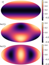 |
Fig. 5 Mollweide projections of the l = 2 spherical harmonics. We evaluate their amplitudes in the Galactic coordinate system, in which the diagram centers and tops are, respectively, (bg, lg) = (0°, 0°) and bg = 90°. With lg decreasing from left to right, the imaginary parts of |


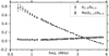 |
Fig. 6 Solutions for b2,0 and Re(b2,2) from Fig. 4 normalized by measurements of the isotropic brightness b0,0 from PSP. Most of the error bars cannot be seen because they do not extend beyond the plot markers. |
4.3 Error and goodness of fit
The error bars in Fig. 4 reflect statistical error in the spectral measurements and uncertainty in the lengths and pointing directions of the antennas. Figure 1 shows the nominal mechanical pointing directions, which are accurate to within 1°. The b2,m solution only depends on the antenna lengths nontrivially through their ratio, whose mechanical value is L34/L12 = 0.9877.
If these parameters for the antenna system are adopted, the average reduced χ2 of the best-fit spherical harmonic model over the entire frequency band is  . Here, χ2 at a given frequency is an average of the squared deviation of the spectral data yi,j from the model
  in units of the standard errors σi,j quoted in Sect. 2.2,
  , where j indexes time, i indexes the types of spectra, and S = 1 or 3.
The overall  exceeds 1 principally because there is a band of heightened χ2 ≈ 1 .09 from 1 to 3 MHz, where the sky is most anisotropic. If the only deviation of the data from the model were due to the statistical spectral measurement error, the occurrence probability of an average value for χ2 as large as 1.09 in this frequency range would be less than 1 × 10⁻⁶. It is more likely that the model does not perfectly describe the data. For example, electrical currents through the spacecraft body can cause the effective antenna height vectors to diverge from the mechanical vectors. The resulting deviation of the data from the spherical harmonic model will be larger at frequencies where the sky is more anisotropic, and when the deviation is comparable to the standard errors σi,j, anon-negligible increase in χ2 results.
If the effective antenna vectors were to diverge from the mechanical ones while the antennas nevertheless acted as ideal short dipoles, the spherical harmonic analysis could be used to solve for both the l = 2 coefficients and the antenna vectors. However, for our data this expanded fit yielded again a  , which indicated that the noise in the measurements was not entirely mitigated or that the antennas did not act exactly as short dipoles.
We therefore did not attempt to constrain the antenna parameters using the data. Because no set of parameters would yield a completely accurate solution for the l = 2 coefficients under the dipole model, we computed solutions for a range of parameters that were randomly selected from Gaussian likelihoods centered on the parameters’ mechanical values. Each antenna’s pointing direction was parameterized by angles of rotations about the spacecraft  -axis and the antenna vector
  cross
cross  axis, both of which were taken to have a standard deviation of 2°. For the antenna length ratio a standard deviation of 0.02 was used. The inflation of these values beyond the mechanical uncertainty accommodated possible electrical perturbations to the antenna response.
We drew M = 1 × 10⁶ random sets of antenna parameters from these distributions. Each set corresponded to a five-dimensional Gaussian solution to the l = 2 coefficients at each frequency ν, say with means µv,i and standard deviations σν,i where i indexes the antenna parameter sets. Here, σν,i is the statistical uncertainty propagated from the error on each data point indicated in Sect. 2.2. The overall solution at a given frequency is the mean of the Gaussian centers,  . Both the spread in the centers of the Gaussians
  and the standard deviations of each Gaussian
  . contribute to the overall error. At most frequencies and for most of the spherical harmonic coefficients, these two contributions are about the same in magnitude.
Lastly, the total uncertainty Πν also includes a fractional error 2 × σL/L ≈ 0.06 due to division by squared effective length in the conversion to units of specific intensity,
![Mathematical equation: $\prod\nolimits_v { = {{\left( {{M^{ - 1}}\sum\limits_i {\left[ {\sigma _{v,i}^2 + {{\left( {{\bf{\mu }}{ & _{v,i}} - - {{{\bf{\bar \mu }}}_v}} \right)}^2}} \right] + 4{{\left( {{{{\sigma _L}} \over L}} \right)}^2}{\bf{\bar \mu }}_v^2} } \right)}^{{1 \mathord{\left/{\vphantom {1 2}} \right.\kern-\nulldelimiterspace} 2}}}.} $](/articles/aa/full_html/2022/12/aa44621-22/aa44621-22-eq61.png) (19)
(19)
5 Modeling free-free absorption
5.1 Outline
To further investigate the compatibility of our results with freefree absorption effects, we generated synthetic low frequency brightness maps and compared their l = 0 and l = 2 expansion coefficients with those measured by PSP. The brightness B at longitude 1g and latitude bg was taken to be
 (20)
(20)
where ε is emitted power per unit volume per unit solid angle per unit frequency bandwidth, s is distance along the line of sight, and τ is optical depth. In the frequency band of our results, the optical depth is determined mostly by free-free absorption. Assuming that the absorbing material consists of ionized hydrogen of uniform temperature, the optical depth to distance d is
 (21)
(21)
where the emission measure  ds with ne in units of cm−3 and s in units of parsecs (Verschuur & Kellermann 1988, p. 41).
From pulsar signals, the dispersion measure DM ≡ ∫ ne ds is known for ~200 paths through the Galaxy ranging in length from ~0.1 kpc to ~10 kpc. It has been found that these data conform to a model of free electrons that includes the disks described in Sect. 4.2, spiral arms, and localized features such as a density enhancement in the Gum Nebula (e.g., Cordes & Lazio 2002; Yao et al. 2017).
Synthetic dispersion measures  ds generated from the model electron densities
  typically reproduce empirical dispersion measures. However, smaller scale density fluctuations are superimposed on the average spatial variation captured by these models, causing
  ds to underestimate the true emission measure. The finer scale structure is often taken to include clumping of the plasma into discrete clouds, say with densities Ne (e.g., Cordes & Lazio 2002). Assuming that the density is uniform within each cloud, EM depends on the fraction η of the total volume occupied by clouds and the cloud-to-cloud variation in the internal densities. Specifically, with
  where the brackets indicate, for a line of sight through the volume, an average over the portion of the line of sight that is occupied by clouds, EM can be approximated as
  ζd s.
ζd s.
Additionally allowing for density fluctuations within each cloud with the same fractional variance  in all clouds, the emission measure increases to EM =
  ds. The same definition of ζ holds here as in the absence of fluctuations, but the densities Ne are now the mean in each cloud. Under the hypothesis that the wavenumber spectrum of the intra-cloud fluctuations assumes a power-law with index −β between an inner scale 11 and outer scale 10 ≫ 11, pulsar signal scattering measurements can be used to determine
  . In the model of Cordes & Lazio (2002), hereafter referred to as NE2001, the Kolmogorov value 11 / is taken for β Using the fluctuation parameters
  included in NE2001, the emission measure is given by
 (22)
(22)
Based on measurements of DM and EM, respectively, the spatial averages of density  and squared density
  in the thick disk have been found to decrease exponentially with distance z from the plane. Gaensler et al. (2008) compared these measurements to assess
  and found
 (23)
(23)
with a = 0.04 ± 0.01.
Limitation of the EM data to Galactic latitudes ∣bg∣ < 35° caused the restriction ∣z∣ < 1.4 kpc in this result, and Gaensler et al. (2008) argued that at ∣z∣ ≳ 2 kpc, f likely decreases unti reaching f ≈ 0.02 at ∣z∣ ≈ 5−10 kpc. Because the average density  is relatively small here, the resulting change in absorptivity would have a negligible impact on the brightness distribution at the resolution of dipole antennas. For this reason, we simply used a constant value f (z) = ae2 at ∣z∣ > 1.4 kpc.
With l0 taken to be 1 pc,  for the thick disk in NE2001. This is much smaller than f−1, whose minimum is 3.4, which suggests that f is mostly determined by the inter-cloud spatial structure, f ≈ ηζ−1. The use of the term “filling factor” for f is therefore appropriate here. However, in some regions of the Galaxy, turbulent fluctuations become prominent. For the Galactic center, for example,
  in NE2001, again with the assumption that l0 = 1 pc.
When evaluating EM, we used the average density  given by the model of Yao et al. (2017), hereafter referred to as YMW16. To account for smaller scale features of the thick disk, we used the form for f in Eq. (23) with a = 0.04. For f of the remaining components, we approximated η−1 ζ = 2 and l0 = 1 pc and used values for F such that
  was roughly consistent with NE2001. Namely, we took f−1 = 7 for the thin disk, f−1 = 3 for the spiral arms, f−1 = 1 × 10⁵ for the Galactic center, and f−1 = 2 for all other components.
For the synchrotron emissivity in the Galaxy ɛsyn, we adopted the cylindrically symmetric model from Eq. (17) of Cong et al. (2021). It was derived by fitting the Haslam et al. (1982) 408 MHz full sky map with free-free and extragalactic emission subtracted to  , where the upper limit of the integral dg(lg, bg) is the distance to the edge of the Galaxy. Free-free absorption is expected to be negligible at 408 MHz, so can be ignored.
Table 2 presents the bl,m coefficients of the Haslam et al. (1982) map along with those of the model map  , where TE is an assumed isotropic extragalactic background and Tff is the contribution from free-free emission. Both the empirical mean brightness and
  anisotropy are well reproduced by the model. Improvements that decrease the discrepancies in the remaining coefficients can be the subject of future work.
With descending frequency, visibility is restricted to progressively closer sources of radiation. Surveys of this modified sky provide information about the distribution of Galactic emissivity that is distinct to the information from the 408 MHz map. Bassett et al.(in prep.) accordingly fit for the distribution along with absorption parameters in their analysis of the PSP measurements. More conservatively, we compared the observed evolution of the brightness distribution with the expected imprint of absorption on the Cong et al. (2021) model.
The emissivity was taken to have a power-law form in frequency with a temperature spectral index β = −2.51. Its increase with decreasing frequency caused it to exceed the free-free emissivity by several orders of magnitude in the frequency band of our results, so we ignored free-free emission. Our analysis does not tightly constrain the extragalactic background, but shows the compatibility of the data with the isotropic brightness temperature TE(v) = 1.2(v/(1 GHz))−258 K used by Cong et al. (2021). The free-free optical depth to these emissions consists primarily of the contributions from the Galaxy and from the circumgalactic medium (CGM, Cong et al. 2021). For the assumed form of TE(v), we find that an isotropic τCGM = τCGM.0(v/(1 MHz))−21 with τCGM,0 < 0.5 produces good agreement between the synthetic bl,m and the data. We adopted τCGM,0 = 0.2 in the results that are shown.
In full, the model maps were evaluated according to
 (24)
(24)
with θ denoting the arguments (lg, bg,v) and where τ(θ, s) was determined using Eq. (21) with EM integrated out to distance s along the line of sight (lg, bg). For simplicity, the electron temperature was assumed to be uniform at 8000 K (Ferrière 2001).
Spherical harmonic expansion coefficients at 408 MHz.
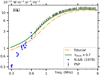 |
Fig. 7 Mean intensity of the real brightness distribution and the synthetic distributions described in the text. |
5.2 Compatibility with observations
Figure 7 presents comparisons between the average intensity of the synthetic and observed brightness distributions. The results from the model described in Sect. 5.1 are labeled “fiducial,” and the results labeled “τthick × 0.7” show the impact of a decrease in the absorptivity of the thick disk by a factor of 0.7. This change could arise, for example, from an increase in a in Eq. (23) to a = 0.05 along with a rise in the gas temperature to ≈9000 K.
Both models fail to reproduce the Novaco & Brown (1978) measurements at v < 0.6 MHz, where there is a deficit in empirical brightness relative to that expected from power-law radiation counteracted by free-free absorption. Peterson & Webber (2002) made the same observation and invoked an electron cloud centered on the Solar System that absorbs the surplus model flux, but no such feature is included in YMW16. Alternatively, Brown (1973) hypothesized that the synchrotron emissivity becomes suppressed due to dispersive effects in the emitting plasma at frequencies that do not greatly exceed the plasma frequency, ν  vpe. For typical magnetic field, relativistic electron, and plasma parameters, this can result in a turnover in the emissivity between 0.1 and 1 MHz (Ramaty 1972), which is consistent with our and prior analysis of the low frequency spectrum.
We focus on frequencies ν > 0.6 MHz, where the observed mean brightness and l = 2 anisotropy are compatible with power-law synchrotron emissivity. Here, the spectral indices dlog /d log(v) of the fiducial model and empirical means differ by at most 0.3 as they evolve from ≈0 to ≈1.8 with decreasing frequency. Even so, a ≈10% error in the model at 5 MHz increases to ≈30% at 0.7 MHz because the difference in trends is systematic. The τthick × 0.7 results indicate the possible origination of the discrepancy in excess thick disk absorptivity, the reduction of which yields a mean brightness that is equal to the true mean to within 10% at all ν > 0.7 MHz.
Figure 8 shows that this model also more accurately captures the empirical b2,0 coefficient than the fiducial model. With declining frequency at ν ≳ 1.5 MHz, preferential extinction at ∣bg∣ < 35° causes b2,0 to increase. However, near ν = 1 MHz, the propagation distance s through which radiation becomes very attenuated, say e−τ(s) < 0.01, comes to be comparable with the thick disk’s height. This marks a transition in the free-free absorption pattern towards isotropy, which leads to the fall in b2,0 at lower frequencies. The diminished absorptivity in the τthick × 0.7 model causes a decline in the turnover frequency, and the higher synchrotron emissivity here results in a higher b2,0 peak. Both of these shifts reduce discrepancies with the measured b2,0 at ν < 1.6 MHz.
The Re(b2,2) results indicate that a concentration of brightness at ∣lg ∣ < 45° persists to lower frequencies in the true brightness distribution than in the synthetic distributions, which is possibly caused by excess model absorption at these longitudes. Further decreases in the thick disk optical depth cannot correct the error because they do not cause Re(b2,2) to increase at all frequencies. Other candidate components of the free electron model include the thin disk and the spiral arms. We find that modifications to the thin disk have only a marginal impact on the l = 2 coefficients at ν < 7 MHz. Also, the results labeled “τarms ÷ 3” demonstrate that even an extreme reduction in the spiral arm optical depth, in this case by a factor of 3, does not reconcile the model Re(b2,2) with the data.
Alternatively, the inconsistency may originate in the model emissivity distribution, which is shown in Table 2 to not accurately capture the  anisotropy of the true emissivity. This is in part caused by asymmetric emission features such as Loop I. Some adopt the view that Loop I is located a few hundred parsecs from the Solar System (e.g., Yao et al. 2017), in which case the relatively small optical depth to it would enhance its prominence at low frequencies and cause the disagreement between the model and true emissivities to worsen.
The absence of such asymmetric emission in the model and the symmetries of the  and
and  spherical harmonics cause b2,1 and Im(b2,2) to be zero at 408 MHz to within a small tolerance arising from the Solar System’s offset from the Galactic plane. These model coefficients remain approximately zero until signatures of asymmetric absorption emerge at ν ≈ 20 MHz. For example, Re(b2,1) is predominantly influenced by density enhancements and depletions within a few hundred parsecs of the Solar System, without which its magnitude remains less than 0.4 × 10⁻²¹ W m−2 sr−1/2 Hz−1 at all frequencies.
In the 0.5 < ν < 7 MHz band of Fig. 8, the trend of this model coefficient with frequency resembles the trend in the empirical coefficient. However, there is a negative offset in the observed Re(b2,1), which is probably in part caused by emission enhancements in (∣lg∣ < 90°, bg > 0°) that are evident at 408 MHz. Conclusive interpretation of the Re(b2,1) measurement will require inclusion of such features in the emission model, which could reduce the offset while preserving the correlation and thereby provide evidence for the local components of the YMW16 density model.
The Im(b2,1) and Im(b2,2) measurements cannot be similarly decomposed into possible imprints of asymmetric absorption and contributions from asymmetric emission. Increasing prominence of local emission irregularities with decreasing frequency, dependence of the synthetic absorption signatures on a flawed emission model, and errors in the adopted free electron distribution may all play a role in the lack of correlation between the synthetic results and the data here.
The model still accurately captures the evolution in the mean brightness and the dominant l = 2 anisotropy over a decade of frequency using a free electron distribution derived from independent measurements. This confirms synchrotron emission with a spectral index β ≈ −2.5 and free-free absorption to be the principal mechanisms of Galactic radiation transfer in 0.6 < ν < 7 MHz. Bassett et al.(in prep.) analyze the PSP data using a Bayesian nested sampling algorithm in order to more methodically constrain the Galactic emissivity and absorptivity.
Decreasing τCGM to 0 in the model raises the height of the b2,0 peak by ≈1 × 10⁻²¹ Wm−2 sr−1/2 Hz−1 and negligibly affects the other coefficients. This does not decisively alter the overall agreement between model and data, so our results have little implication for radiation transfer outside the Galaxy. It is possible that the CGM remains transparent at these frequencies, or that the extragalactic background is much smaller than what we approximated and that most of this radiation is actually Galactic.
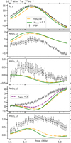 |
Fig. 8 Spherical harmonic expansion coefficients of the empirical brightness distribution and the synthetic distributions described in the text. |
6 Conclusions
Between 0.5 and 7 MHz, PSP’s antennas approximately act as short ideal dipoles. As a result, their measurements of the radio background are linear combinations of the background’s l = 0 and l = 2 spherical harmonic expansion coefficients. We fit the data to this model with an average reduced  across the analyzed frequency band. The best-fit coefficients reveal an anisotropic evolution of the brightness distribution with frequency, which contrasts with the approximately isotropic power-law evolution seen at higher frequencies. In particular, the l = 2, m = 0 coefficient shows a darkening of the Galactic plane relative to the poles with decreasing frequency.
This is an expected effect of free-free absorption because the associated ionized gas is concentrated in the Galactic plane. Such spatial variation in the gas density is captured in model free electron distributions derived from pulsar measurements. We used one of these distributions, YMW16, to make quantitative predictions for the resulting anisotropic attenuation that could be compared with the PSP measurements. Specifically, we generated synthetic low frequency brightness maps using YMW16 for evaluation of the free-free optical depth through the Galaxy.
At ν > 0.6 MHz, the empirical mean brightness and l = 2, m = 0 coefficient can be reproduced in model maps in which the Galactic emissivity maintains a power-law form. In the ν ~ 10 MHz regime, the increasing absorptivity of the interstellar medium with decreasing frequency starts to conceal the coinciding increase in emissivity. Radiation from low latitudes is preferentially extinguished due to the enhanced density of absorbing gas in the Galactic plane, causing the plane to become generally less bright than the poles at ≈4 MHz. With descending frequency below ≈3 MHz, the power-law increase in emissivity is completely offset by the rising free-free optical depth and the mean sky brightness decreases.
In agreement with prior analyses, we find that the empirical brightness at ν < 0.6 MHz is more strongly suppressed than free-free absorption calculations predict. The free electron distribution that we employed is consistent with pulsar dispersion measures and is able to explain the evolution of the brightness distribution between 0.6 and 7 MHz, so is likely not responsible. Instead, the discrepancy may point to a deviation of the synchrotron emissivity from a power-law at ν ≲ 0.6 MHz.
Acknowledgements
The FIELDS instrument and Parker Solar Probe are funded under task order NNN10AA08T of NASA contract NNN06AA01C. Development of the spacecraft was led by the Johns Hopkins Applied Physics Laboratory. Institutions that contributed to the design and assembly of the FIELDS instrument are noted on the “Team” page of https://fields.ssl.berkeley.edu. The data used in this study can be accessed from the “Data” page of the same web site. The work of NB was supported by the NASA Solar System Exploration Research Virtual Institute cooperative agreement number 80ARC017M0006. This study was also partially supported by the Universities Space Research Association via DR using internal funds for research development. DR’s work was also in part funded by NASA grant 80NSSC23K0013.
References
- Acton, C., Bachman, N., Semenov, B., & Wright, E. 2018, Planet. Space Sci., 150, 9 [Google Scholar]
- Alexander, J., Brown, L., Clark, T., & Stone, R. 1970, A&A, 6, 476 [NASA ADS] [Google Scholar]
- Balanis, C. 1992, Proc. IEEE, 80, 7 [NASA ADS] [CrossRef] [Google Scholar]
- Bale, S. D., Goetz, K., Harvey, P. R., et al. 2016, Space Sci. Rev., 204, 49 [Google Scholar]
- Brillinger, D. R. 2001, Time Series: Data Analysis and Theory (USA: Society for Industrial and Applied Mathematics) [CrossRef] [Google Scholar]
- Brown, L. W. 1973, ApJ, 180, 359 [NASA ADS] [CrossRef] [Google Scholar]
- Cong, Y., Yue, B., Xu, Y., et al. 2021, ApJ, 914, 128 [NASA ADS] [CrossRef] [Google Scholar]
- Cordes, J. M., & Lazio, T. J. W. 2002, ArXiv preprint [arXiv:astro-ph/0207156] [Google Scholar]
- Ellis, G. R. A. 1982, Australian J. Phys., 35, 91 [NASA ADS] [CrossRef] [Google Scholar]
- Ellis, G. R. A., Waterworth, M. D., & Bessell, M. 1962, Nature, 196, 1079 [NASA ADS] [CrossRef] [Google Scholar]
- Ferrière, K. M. 2001, Rev. Mod. Phys., 73, 1031 [NASA ADS] [CrossRef] [Google Scholar]
- Fox, N. J., Velli, M. C., Bale, S. D., et al. 2015, Space Sci. Rev., 204, 7 [Google Scholar]
- Gaensler, B. M., Madsen, G. J., Chatterjee, S., & Mao, S. A. 2008, PSAA, 25, 184 [Google Scholar]
- Guzmán, A. E., May, J., Alvarez, H., & Maeda, K. 2010, A&A, 525, A138 [Google Scholar]
- Haslam, C. G. T., Salter, C. J., Stoffel, H., & Wilson, W. E. 1982, A&AS, 47, 1 [NASA ADS] [Google Scholar]
- Hoyle, F., & Ellis, G. 1963, Australian J. Phys., 16, 1 [NASA ADS] [CrossRef] [Google Scholar]
- Lecacheux, A., & Maksimovic, M. 2019, in Proceedings of JS19 URSI-France, Observatoire de Versailles/Saint-Quentin en Yvelines, 16 [Google Scholar]
- Manchester, R. N., & Taylor, J. H. 1981, AJ, 86, 1953 [NASA ADS] [CrossRef] [Google Scholar]
- Manning, R., & Dulk, G. A. 2001, A&A, 372, 663 [NASA ADS] [CrossRef] [EDP Sciences] [Google Scholar]
- Meyer-Vernet, N. 1979, J. Geophys. Res., 84, 5373 [Google Scholar]
- Moncuquet, M., Meyer-Vernet, N., Issautier, K., et al. 2020, ApJS, 246, 44 [Google Scholar]
- Novaco, J. C., & Brown, L. W. 1978, ApJ, 221, 114 [NASA ADS] [CrossRef] [Google Scholar]
- Peterson, J. D., & Webber, W. R. 2002, ApJ, 575, 217 [NASA ADS] [CrossRef] [Google Scholar]
- Pulupa, M., Bale, S. D., Bonnell, J. W., et al. 2017, J. Geophys. Res. Space Phys., 122, 2836 [Google Scholar]
- Ramaty, R. 1972, ApJ, 174, 157 [NASA ADS] [CrossRef] [Google Scholar]
- Reber, G., & Ellis, G. R. 1956, J. Geophys. Res., 61, 1 [NASA ADS] [CrossRef] [Google Scholar]
- Remazeilles, M., Dickinson, C., Banday, A. J., Bigot-Sazy, M.-A., & Ghosh, T. 2015, MNRAS, 451, 4311 [Google Scholar]
- Shain, C. 1954, Australian J. Phys., 7, 150 [NASA ADS] [CrossRef] [Google Scholar]
- Taylor, J. H., & Cordes, J. M. 1993, ApJ, 411, 674 [Google Scholar]
- Verschuur, G. L., & Kellermann, K. I., eds. 1988, Galactic and Extragalactic Radio Astronomy (New York: Springer) [CrossRef] [Google Scholar]
- Yao, J. M., Manchester, R. N., & Wang, N. 2017, ApJ, 835, 29 [NASA ADS] [CrossRef] [Google Scholar]
- Zaslavsky, A., Meyer-Vernet, N., Hoang, S., Maksimovic, M., & Bale, S. D. 2011, Rad. Sci., 46, RS2008 [Google Scholar]
All Tables
All Figures
|
Fig. 1 Antenna system of PSP. The four sensors V1, V2, V3, and V4 are mounted to and coplanar with the spacecraft heat shield, which is located in the back of the diagram. Radiator fins extend from the heat shield to a 1.5 m long hexagonal spacecraft bus in the foreground. The |
| In the text | |
|
Fig. 2 Amplitudes of the Galactic background, thermal electronic noise, and quasi-thermal noise in the RFS auto spectra. |
| In the text | |
|
Fig. 3 Mean sky intensity measurements from PSP scaled to data from Novaco & Brown (1978) using effective antenna lengths, L12 = 3.3 ± 0.1 m and L34/L12 = 0.99 ± 0.01, that minimize the summed squared residuals between the data sets. The relative uncertainty on most of the Novaco & Brown (1978) points is between 15 and 20%. |
| In the text | |
|
Fig. 4 Spherical harmonic expansion coefficients of the radio brightness distribution between 0.5 and 7 MHz. Section 4.3 describes the sources of uncertainty in the results. |
| In the text | |
|
Fig. 5 Mollweide projections of the l = 2 spherical harmonics. We evaluate their amplitudes in the Galactic coordinate system, in which the diagram centers and tops are, respectively, (bg, lg) = (0°, 0°) and bg = 90°. With lg decreasing from left to right, the imaginary parts of |
| In the text | |
|
Fig. 6 Solutions for b2,0 and Re(b2,2) from Fig. 4 normalized by measurements of the isotropic brightness b0,0 from PSP. Most of the error bars cannot be seen because they do not extend beyond the plot markers. |
| In the text | |
|
Fig. 7 Mean intensity of the real brightness distribution and the synthetic distributions described in the text. |
| In the text | |
|
Fig. 8 Spherical harmonic expansion coefficients of the empirical brightness distribution and the synthetic distributions described in the text. |
| In the text | |
Current usage metrics show cumulative count of Article Views (full-text article views including HTML views, PDF and ePub downloads, according to the available data) and Abstracts Views on Vision4Press platform.
Data correspond to usage on the plateform after 2015. The current usage metrics is available 48-96 hours after online publication and is updated daily on week days.
Initial download of the metrics may take a while.